Parameter Studies on Hydraulic Fracturing in Brittle Rocks Based on a Modified Hydromechanical Coupling Model

Abstract

In this paper, we present a numerical study of hydraulic fracturing in brittle rock by using particle flow simulation. The emphasis is put on the influence of in situ stress, differential stress, fluid injection rate, fluid viscosity and borehole size on hydraulic fracturing behavior. To this end, an improved hydromechanical coupling model is first introduced to better describe fluid flow and local deformation of particle-based rocks. A series of parameter sensitivity studies are then conducted under the framework of particle flow simulation. Modelling results suggest that the breakdown pressure and time to fracture both linearly increase with confining stress, and hydraulic fracturing patterns present a distinct transition from brittle to ductile. Fluid injection rate and fluid viscosity have similar influences on hydraulic fracturing propagation, their value decrease leads to borehole pressure decrement and time to fracture prolongation. However, the former mainly controls the time to initial cracking, while the latter largely decides the duration of fracturing propagation. As for borehole radius, its increases can directly enhance the fluid diffusion zone, which further intensifies the nonlinear property of borehole pressure, leads to breakdown pressure decrease, prolongs time to fracture and forms more complex hydraulic fractures.

1. Introduction

Hydraulic fracturing has been widely employed in the energy industry as a technique that creates a desired fracture network to increase energy production [1,2], for instance, in petroleum and gas enhancement. Initiation and propagation of fluid-driven fracture often present an extremely complex process due to the uncertainty during fluid pressurization. Many factors [3,4,5], such as the in situ stress states, fluid injection rate, fluid viscosity and fluid injection borehole, can affect hydraulic fracturing behavior in terms of fluid breakdown pressure, fluid diffusion ability and fracture propagation pattern. It is still necessary to increase understanding of the influence of these factors to improve the implementation of fracturing design.

A large number of experimental studies have been performed to investigate hydraulic fracturing propagation in rocks with the help of uniaxial and true triaxial tests considering fluid injection [6,7,8]. Different types of cylindrical/cubic rock samples with or without pre-existing fissures are considered [9,10,11,12]. Effects of factors including confining stress, fluid injection rate, borehole diameter and pre-existing fracture are also studied. It is not an easy task to give an exhaustive review of all previous studies. Most of them show that the borehole pressure response and hydraulic fracture pattern have an obvious dependency on local stress evolution around the borehole. This stress evolution is actually determined by the combined role of ambient stress, fluid injection and borehole features.

In order to describe hydraulic fracturing behavior under different factors, analytical and semi-analytical studies endeavour to propose the corresponding breakdown pressure criterion to predict initial hydraulic fracture propagation by calculating fluid-induced stress values around the borehole. For instance, some different simplified solutions [13,14,15,16] have been proposed under the frame of effective stress theory with the assumption that the rock matrix is a homogeneous elastic medium and no fluid diffusion exists between the borehole and rock matrix. In these solutions, the borehole breakdown pressure is often regarded as a function of ambient stress and rock strength. However, in numerous experiments, different fluid-injection and confining stresses often result in different breakdown pressure as well as fracture modes [17]. Therefore, the description for breakdown pressure response and hydraulic fracture propagation under different influence factors is still an open issue.

Numerical simulation analysis has been developed largely as alternative approaches, in both continuous and discontinuous categories. Among the discontinuous approaches, the discrete element method is one of the most widely used ones, especially for the Particle Flow Code (PFC) [18,19,20,21,22,23]. In this method, the continuum rock mass is replaced by an assembly of bonded discrete particles. The overall deformation and failure are essentially controlled by the local behavior of bonded interfaces. Recently, by introducing a fluid network model at bonded contacts between particles, this method has been further extended to handle the hydraulic–mechanical coupled category [24,25,26,27,28]. A large number of attempts have been conducted to simulate the hydraulic fracturing process in either intact or fractured rocks under different confining stresses [29,30,31,32,33,34]. However, most of previous simulations only focused on descriptions of final fracture patterns [33,35,36,37]. Few of them pay attention to quantitative variation in breakdown pressure versus fluid parameters and in situ stress, which is also essential to analyze hydraulic fracturing behavior under different influence factors.

The reason for this is that previous studies have generally adopted the same fluid network model, which was originally embedded in particle flow code (PFC). In this model, hydraulic aperture evolution is regarded as a linear function of normal stress at contacts. It cannot accurately describe fluid flow and local deformation during the hydraulic-coupling process. As a consequence, a more precise fluid network model has been proposed in our previous study [34] that defines hydraulic aperture as an empirical function of normal stress as well as bond breakage. Therefore, here we will still adopt this model. The emphasis in this paper is put on further investigation of the effect of different factors on hydraulic fracturing behavior.

The present study is organized as follows. An improved fluid network model is first introduced and numerical calibration on model parameters is conducted. After a series of hydraulic fracturing simulations, parameter sensitivity studies including in situ stress, differential stress, fluid injection rate, fluid viscosity and borehole size are then completed. The obtained results are used to further investigate the influence of these underlying factors on hydraulic fracturing behavior in terms of borehole pressure and fracture propagation.

The following sign convention will be adopted throughout the paper. The compressive normal stress is denoted as a positive value and the tensile normal stress as a negative one.

2. Hydraulic Coupling Methodology

In fluid coupling analysis with particle flow simulation, the overall deformation and fracture propagation are essentially controlled by the local behavior of inter-granular interfaces, which is closely related to the bond model and fluid network model applied at contact interfaces. In this regard, while thorough details on the fundamental hydromechanical algorithm have been presented by numerous authors in the literature [38,39,40], only a brief introduction is given as follows.

2.1. Contact Stiffness Behavior

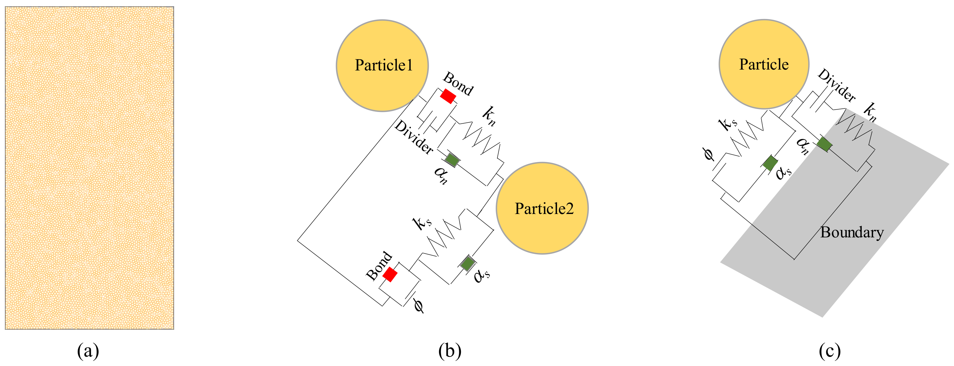
In calculation of local stresses at contacts (particle–particle or particle–boundary, Figure 1), a simple linear contact stiffness model is used to describe the local elastic behavior of rock materials. The detailed force-displacement relations can be expressed as follows:

$$F_n=k_n{u}_n$$

(1)

$$\Delta F_s=-k_s\Delta u_s$$

(2)

where, $F_n$, $k_n$ and $u_n$ are, respectively, the normal force, normal stiffness and displacement at the contact; $\Delta F_s$, $k_s$ and $\Delta u_s$ denote, respectively, the shear force, shear stiffness and relative displacements in each time step $\Delta t$. Note that the normal stiffness, $k_n$, is a secant modulus that relates to the total displacement and force. The shear stiffness, $k_s$, on the other hand, is a tangent modulus that relates to the incremental displacement and force.

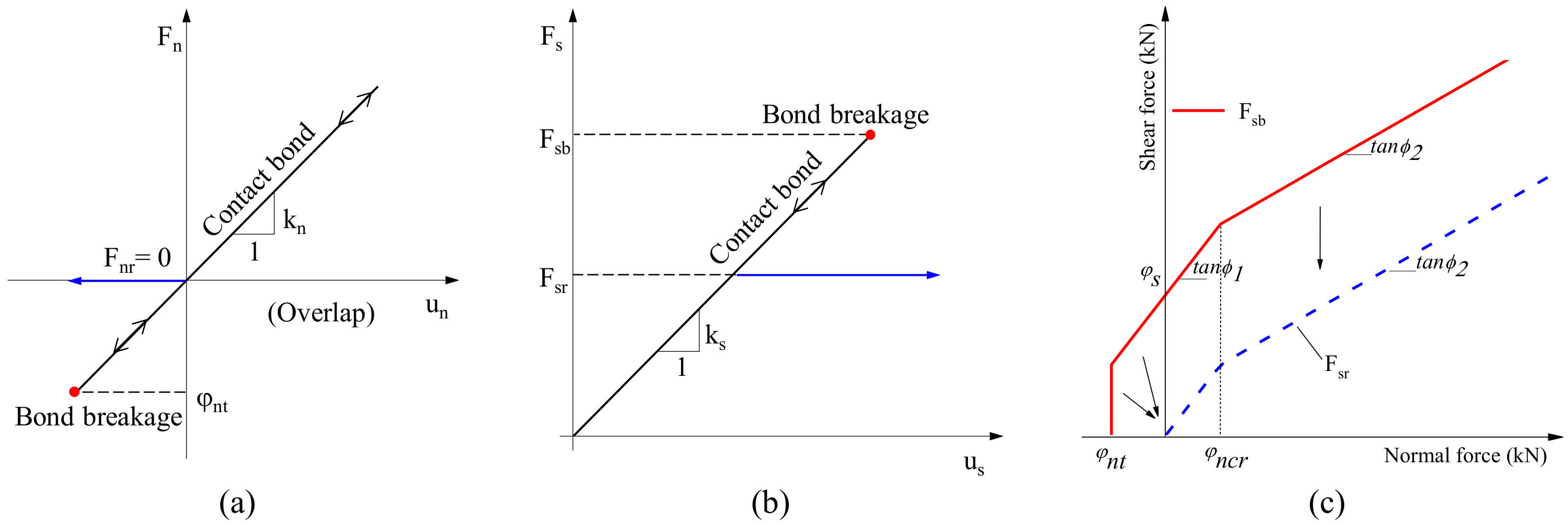
2.2. Contact Bond Behavior

When local stress at the contact reaches a critical value, the contact bond is broken. This process is related to the bond model applied at the contact. Two typical bond models, i.e., the contact bond model (CBM) and parallel bond model (PBM), are often used in particle flow simulations. Due to a simple linear strength failure criterion embedded, these two bond models cannot correctly describe the effect of normal stress on shear strength, especially for a large range of normal stresses. Therefore, in order to better describe the macro mechanic nonlinear property of rocks, a new bond model with nonlinear strength failure criterion has been proposed in our previous studies [41,42], such as that illustrated in Figure 2.

In this bond model, two debonding mechanisms are taken into account: the tensile failure and shear failure. Tensile cracking occurs when the normal contact force $F_{n,f}$ exceeds the normal strength ${\phi }_{nt}$. The shear failure process is relatively more complex, depending on both normal force and tangential shear strength. The shear strength of the interfaces is here approximated by a bi-linear function of normal contact force. When the normal contact force is less than the transition threshold ${\phi }_{ncr}$, the shear strength is defined by the cohesion ${\phi }_s$ and frictional angle ${\varphi }_1$. When the normal force is larger than ${\phi }_{ncr}$, a second frictional angle ${\varphi }_2$ is introduced with ${\varphi }_2<{\varphi }_1$ to define the shear strength. The failure criterion for contact interface is then expressed in the following form:

$$F_{n,f}={\phi }_{nt},\mathrm{tensile}\mathrm{failure}$$

(3)

$$F_{s,f}=\left\{\begin{array}{c}0\hfill \\ {\phi }_s+F_{n}tan{\varphi }_1\hfill \\ {\phi }_s+{\phi }_{ncr}(tan{\varphi }_1-tan{\varphi }_2)+F_{n}tan{\varphi }_2\hfill \end{array}\right.\begin{array}{c}, F_n<{\phi }_{nt}\hfill \\ , {\phi }_{nt}\le F_n\le {\phi }_{ncr}\hfill \\ , F_n\ge {\phi }_{ncr}\hfill \end{array}, \mathrm{shear}\mathrm{failure}$$

(4)

When the contact surface is broken, the tensile strength immediately drops to zero, and the shear strength reduces to a residual value that is a function of the normal force and the coefficient of friction acting on the irregular contact surface. The residual strength envelope is shown in Figure 2c, and the following criterion is formulated:

$$F_{s,r}=\left\{\begin{array}{c}0\hfill \\ F_{n}tan{\varphi }_1\hfill \\ {\phi }_{ncr}(tan{\varphi }_1-tan{\varphi }_2)+F_{n}tan{\varphi }_2\hfill \end{array}\right.\begin{array}{c}, F_n\le 0\hfill \\ , 0<F_n\le {\phi }_{ncr}\hfill \\ , F_n>{\phi }_{ncr}\hfill \end{array}$$

(5)

2.3. Hydraulic Coupling Behavior

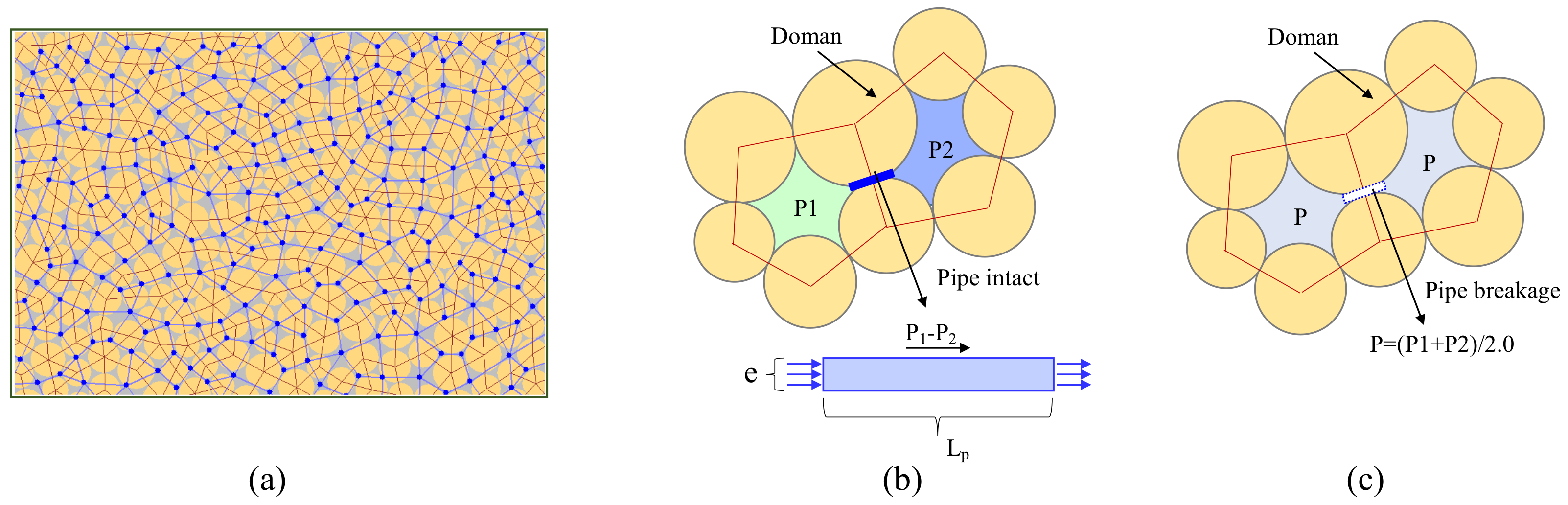
The fluid network model in Figure 3 is mainly composed of two components: the pipes (channels) and domains (reservoirs). Each contact bond serves as one fluid pipe (channel, blue line) linking adjacent domains. A series of enclosed domains (reservoirs, blue points) are created by red lines connecting the centers of neighbouring particles. Each domain (reservoir) has a certain volume and can store some fluid.

When differential pressure between two neighboring domains exists, the corresponding fluid flow happens along their linking pipes. Assuming that each pipe is a set of parallel plates with a certain aperture of e, and fluid flow in the pipe is modelled as laminar, the fluid flow can be calculated using the Poiseuille Equation and the corresponding volumetric laminar-flow rate q can be expressed by:

$$q=\frac{e^3\left(p_1-p_2\right)}{12\mu L_p}$$

(6)

where e is the hydraulic aperture; $L_p$ is the length of fluid pipe; $p_1-p_2$ is the differential pressure between adjacent domains, and $\mu$ is the fluid viscosity.

Correspondingly, for each domain, the flow fluid of surrounding pipes induces a change in its interior fluid volume $\Delta V_d$ as well as fluid pressure $\Delta p$, and that is:

$$\Delta p=\frac{K_f}{V_d}(\sum q\Delta t-\Delta V_d)$$

(7)

$K_f$, $V_d$, $\Delta V_d$ are, respectively, the bulk modulus of the fluid, the domain volume and the change in volume of the domain. After that, the updated fluid pressure of the domain will act on surrounding particles by applying the equivalent body force, thus resulting in variation in the local stress value and hydraulic aperture size e, such as illustrated in Figure 3b.

As mentioned above, during the coupling process, hydraulic aperture evolution plays an important role which controls fluid exchange between adjacent domains. As a consequence, an improved fluid network model has been proposed in our previous studies [34,43]. In this model, hydraulic aperture variation is defined as an empirical function of normal force and bond state at contacts. Its detailed formulations are expressed by the following equations:

$$e=\left\{\begin{array}{cc}{e}_{res}+(e_{ini}-e_{res})exp(-\alpha {\sigma }_n)\hfill & ,\mathrm{compressive}\mathrm{stress}\hfill \\ e_{ini}+\beta \Delta d\hfill & ,\mathrm{tensile}\mathrm{stress}\hfill \end{array}\right.$$

(8)

$e_{ini}$ and $e_{res}$ denote, respectively, the initial and residual aperture of the pipe; $\alpha$, $\beta$ are pipe aperture evolution parameters; ${\sigma }_n$ is the normal force at contact, $\Delta d$ represents the distance between adjacent particles. In addition, that proposed model also take into account the bond state influence on the evolution of fluid pressure. When contact bond between particles is intact, the exchange of fluid flow obeys the formulations mentioned above. Once bond breakage happens, fluid pressure in adjacent domains reallocates instantaneously and takes the average value of their total pressure $p=(p_1+p_2)/2$.

3. Calibration and Assessment of Introduced Model

In this section, the improved hydromechanical coupling model is first implemented in the standard particle flow code (PFC) and then these model micro-parameters are calibrated respectively by numerical compression test and fluid flow test. After that, a series of fluid injection tests are performed to further assess the efficiency of the introduced model by comparing theoretical solutions and typical experimental evidence.

3.1. Identification of Micro-Mechanical Parameters

Prior to performing numerical simulation, there are two distinct types of micro-mechanical parameters that need to be calibrated: the stiffness and strength. As this kind of parameter identification process can be found in a large number of references [30,33], we give a brief and clear introduction here.

The parameter identification is completed by an iterative process. More precisely, for the stiffness and strength parameters, their initial values can be estimated according to empirical relationships between micro-mechanical parameters and macro-mechanical properties, and then the final accurate values can be obtained by conducting numerical tests under different confining stresses (Pc) to iteratively adjust these initial values. The detailed flowchart is presented as below.

$$k_n=4E_{c}R,k_s=k_r{k}_n$$

(9)

$${\phi }_{nt}=4{\sigma }_c{R}^2,{\phi }_s=4{\tau }_c{R}^2$$

(10)

• Given the large values for strength parameters (${\phi }_{nt},{\phi }_s,{\phi }_{ncr},tan{\varphi }_1,tan{\varphi }_2$);
• Calculate the stiffness parameters ($k_n,k_s,k_r$) by using EQ.9;
• Identify the stiffness parameters by following iterative process;

  (a)

  Conduct compression test, and obtain macro elastic value $E_1$;

  (b)

  Compare $E_1$ and $E_0$: if $E_1$ = $E_0$, then go to 4, else go to (c);

  (c)

  Update the stiffness values, and go to (a);

• Calculate the strength parameters (${\phi }_{nt},{\phi }_s$) by using EQ.10;
• Identify the strength parameters by following iterative process;

  (d)

  Conduct compression test, and obtain peak strength $S_1$;

  (e)

  Compare $S_1$ and $S_0$: if $S_1$ = $S_0$, then go to 6, else go to (f);

  (f)

  Update the strength values, and go to (d);

• Compare $E_1$, $E_0$ and $S_1$, $S_0$: if ($E_1$ = $E_0$, $S_1$ = $S_0$), then go to 7, else go to (3 and 5);
• Obtain micro mechanical parameters for one Pc;
• Adjust strength parameters (${\phi }_{ncr},tan{\varphi }_1,tan{\varphi }_2$) with other Pc;
• Complete the micro mechanical parameters calculation.

Based on this process, a rock samples of 150 mm in width and 300 mm in height is generated. The number of particles in the sample is about 10,000, with average radii R of 1.33 mm following uniform distribution. The ratio of the largest radius to the smallest one is 1.66, and the porosity of the sample is about 0.15. This particle size choice can completely meet the size ratio of the particle radius to sample width, largely reducing the particle size effect as reported in reference of [41]. A series of calibrations [10] is then conducted according to the procedure mentioned above, and a set of optical model parameters are given in

Table 1. Mechanical parameters for bond model used in hydraulic fracturing test.

Mechanical Parameters for Bond Model
Normal contact stiffness for test (N/m)	$k_n$	$8.3\times 10^8$
Shear contact stiffness for test (N/m)	$k_s$	$5.2\times 10^8$
Inter-particle coefficient of friction	$tan{\varphi }_1$	1.5
Inter-particle coefficient of friction	$tan{\varphi }_2$	0.5
Normal bond strength (N)	${\phi }_{nt}$	$5.7\times 10^4$
Shear bond strength (N)	${\phi }_s$	$2.1\times 10^5$
The critical normal stress (N)	${\phi }_{ncr}$	$4.2\times 10^5$

.

3.2. Identification of Hydraulic-Related Parameters

The improved hydraulic aperture model needs to calibrate four micro-parameters: the initial and residual aperture of the pipe ($e_{ini}$, $e_{res}$), as well as the pipe aperture evolution parameters ($\alpha$, $\beta$). Inspired by previous studies, the residual value of the pipe $e_{res}$ is strongly depended on the initial aperture $e_{ini}$ and here is taken to be 0.1 times the initial aperture value $e_{ini}$. These two aperture evolution parameters, $\alpha$ and $\beta$, can also be indirectly determined, for instance $2.0\times 10^{-5}$ and 0.5, as reported in reference of [34].

As for the identification of the initial aperture $e_{ini}$, two kinds of procedure can be referred to by empirical method and by numerical fluid flow test. Here, we take a similar approach as mentioned above, of a first estimate according to the empirical relationship, which is then further adjusted by numerical testing. Therefore, based on the large number of numerical simulations of fluid flow, an approximate relationship between macro-permeability k and micro-hydraulic aperture $e_{ini}$ has been developed in previous studies [24,44,45] and its detailed expression is as follows.

$$k=\frac{1}{12V}\sum _{pipes}{L}_p{e_{ini}}^3$$

(11)

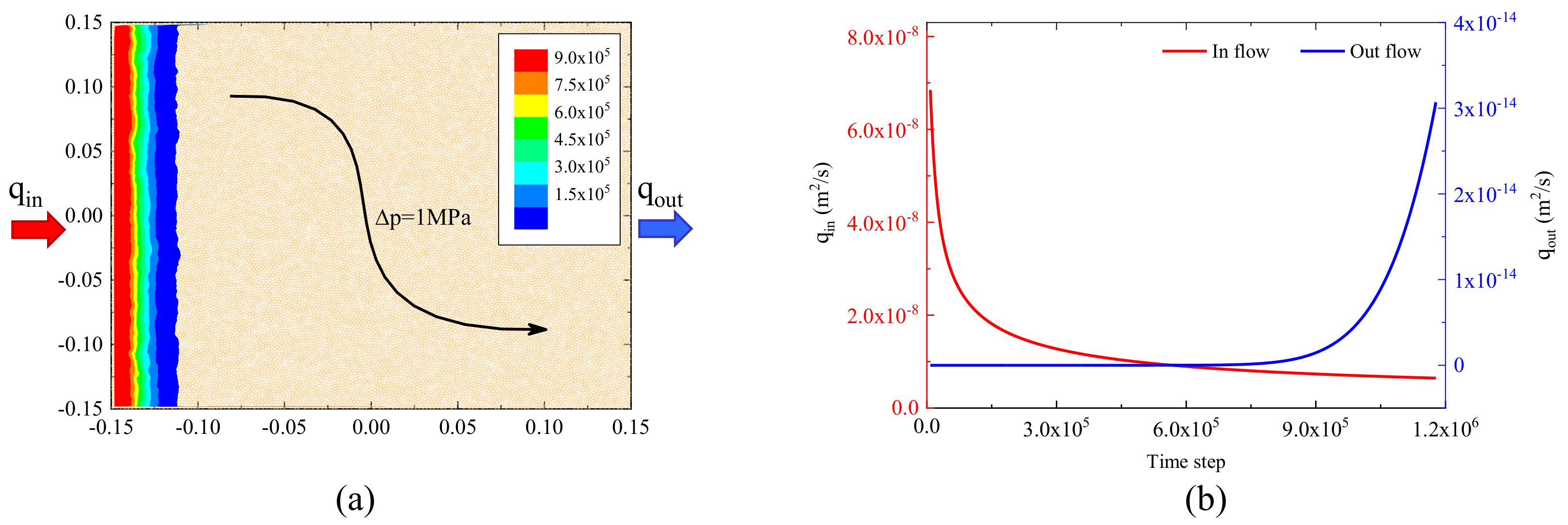
According to the empirical relationship above, an initial hydraulic aperture can be estimated, but its accurate value still needs to be matched iteratively by numerical fluid flow test. The detailed process of this test is as follows. A sample of 300 mm in width (W) and 300 mm in length (H) is first generated, and differential pressure $\Delta p$ of 1 MPa is applied on its two sides, such as shown in Figure 4a. When the input fluid flow rate is equal to that output one ($q_{in}=q_{out}=q_s$), the overall permeability k of the numerical sample can be calculated according to the analysis equation of $k=\left(q_s\mu W\right)/\Delta p$. By comparing permeability obtained numerically and experimentally, the estimated hydraulic aperture is adjusted iteratively. After that, a set of optimal hydraulic related parameters is obtained and given in

Table 2. Hydraulic parameters for fluid network model used in hydraulic fracturing test.

Hydraulic Parameters for Fluid Network Model
Initial hydraulic aperture (m)	$e_{ini}$	$1.6\times 10^{-6}$
Residual hydraulic aperture (m)	$e_{res}$	$0.16\times 10^{-6}$
Model parameters	$\alpha ,$$\beta$	$2.0\times {10}^{-5},$$0.5$
Bulk modulus of the fracturing fluid (GPa)	$K_f$	2.0

. In addition, a typical variation curve of the fluid flow rate is presented in Figure 4b.

3.3. Rock Sample Model and Loading Condition

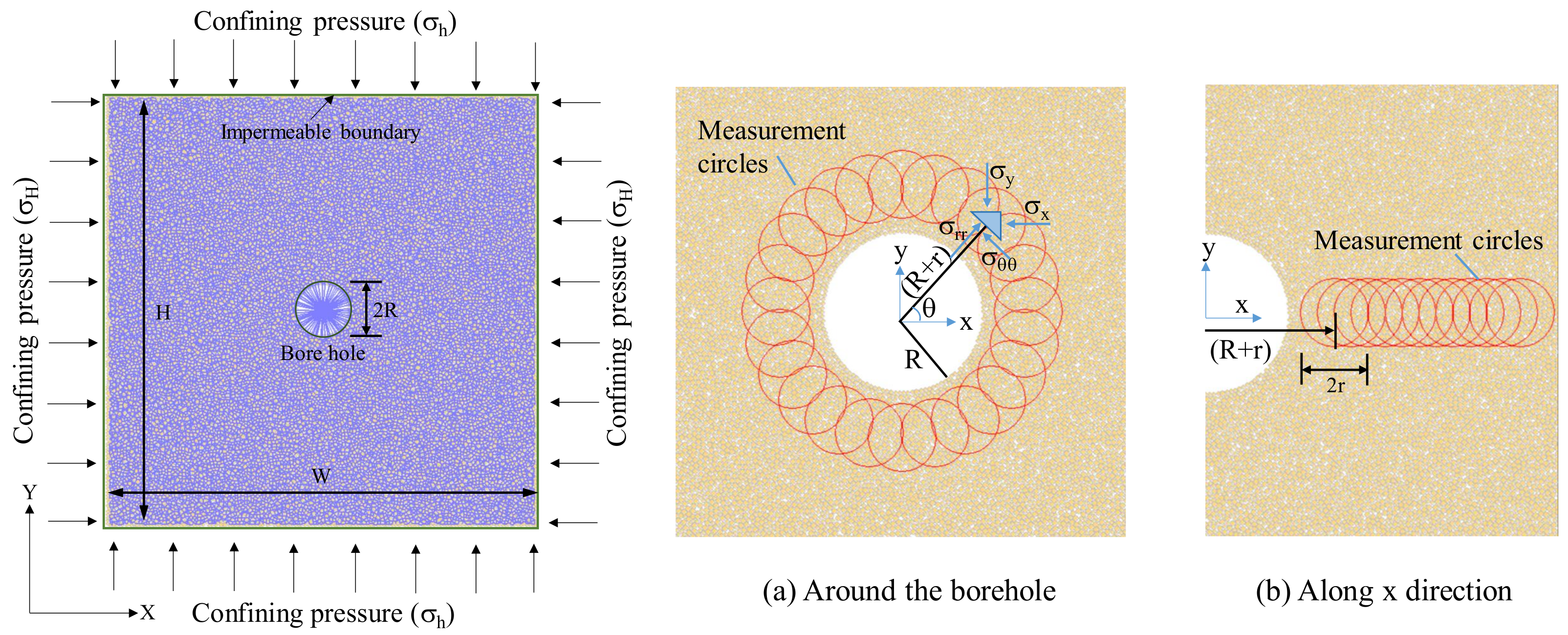
In order to conduct a fluid injection test, a borehole-squared numerical rock sample is first completed. It is 300 mm in width (W) and 300 mm in height (H) with about 20,000 particles. A borehole of 15 mm (R) for fluid injection is created at the center of sample, which is surrounded by some well-organized small particles of 1 mm to possibly eliminate particle heterogeneity causing local stress concentration around borehole. Outside the sample is four moving walls that can apply the specified confining pressure both in x-direction and y-direction. Between those walls and the domain region, there are some un-covered particles to simulate an impermeable rubber housing used in the actual experiment, such as shown in Figure 5. In addition, to obtain stress distribution in the numerical sample and compare with the theoretical stress values, 24 and 16 stress measurement circles with a radius of 15 mm (r) are installed into isotropic numerical samples, respectively around the borehole and along the x direction.

3.4. Assessment of Hydraulic Fracturing Model

Based on the generated borehole-squared rock sample, a series of fluid injection tests are performed to assess the efficiency of the hydromechanical coupling model. For this purpose, two typical cases are considered here: local stress evolution around the borehole, as well as the breakdown pressure variation of the borehole.

3.4.1. Assessment of Local Stress Evolution

By adopting the calibrated parameters in Table 1 and Table 2, and keeping the fluid injection rate of $1.0\times 10^{-5}$ m${}^3$/s, a representative fluid injection test is first carried out with confining stresses of ${\sigma }_H$ = 20 MPa in x direction and ${\sigma }_h$ = 10 MPa in y direction. 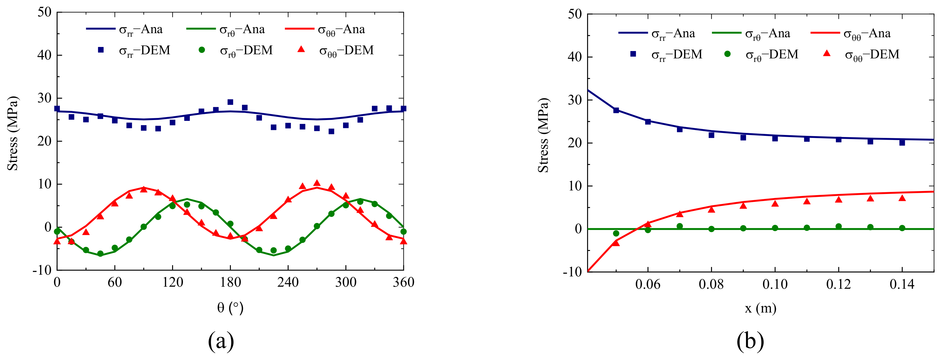During this process, the local stress values, such as the radial (${\sigma }_{rr}$), tangential (${\sigma }_{\theta \theta }$) and shear (${\sigma }_{r\theta }$) stresses around the borehole and along the x direction, can be recorded by those set measurement circles. At the same time, for a circular injection hole in the elastic, homogeneous, isotropic plate, subjected to effective principal stresses, the theoretical values of these local stresses around the hole, as well as along the x direction, can be also obtained according to previous studies [46,47].

Figure 6 first compares local stress evolution induced by fluid injection obtained numerically and theoretically. One can see that the local stress values between them are both in excellent agreement in terms of magnitude and fluctuation characteristics, either around the borehole or along the x direction. More precisely, due to the existence of differential confining stress, the local stress values around the borehole present a gradually concentrated distribution towards x direction. As a result, the tangential stress (${\sigma }_{\theta \theta }$) reaches the maximum (minimum) value when $\theta$ = ${90}^{\circ }$ and ${270}^{\circ }$ ($0^{\circ }$ and ${180}^{\circ }$), and correspondingly the shear one (${\sigma }_{r\theta }$) takes the maximum (minimum) value as $\theta$ equals to ${135}^{\circ }$ and ${315}^{\circ }$ (${45}^{\circ }$ and ${225}^{\circ }$). As for local stress distribution along the x direction, the overall trends for ${\sigma }_{rr}$ and ${\sigma }_{\theta \theta }$ are similar, first sharply changing and then trending to their own gentle values. More notably, due to local stress concentration around the borehole, the tangential stress ${\sigma }_{\theta \theta }$ changes from compression to tension status, which further means the possibility of cracking at the orientation of $0^{\circ }$ and ${180}^{\circ }$ becomes more and more obvious. Therefore, local stress evolution induced by fluid injection can be well reproduced by the introduced hydromechanical coupling model.

3.4.2. Description of Hydraulic Fracturing Behavior

In the modelling of hydraulic fracturing, the description of breakdown pressure is also an important indicator to assess the efficiency of the hydromechanical model. As a consequence, some additional hydraulic fracturing simulations are performed with confining stress(${\sigma }_h$) range of 10 Mpa to 20 Mpa. Other input parameters remain unchanged as mentioned above.

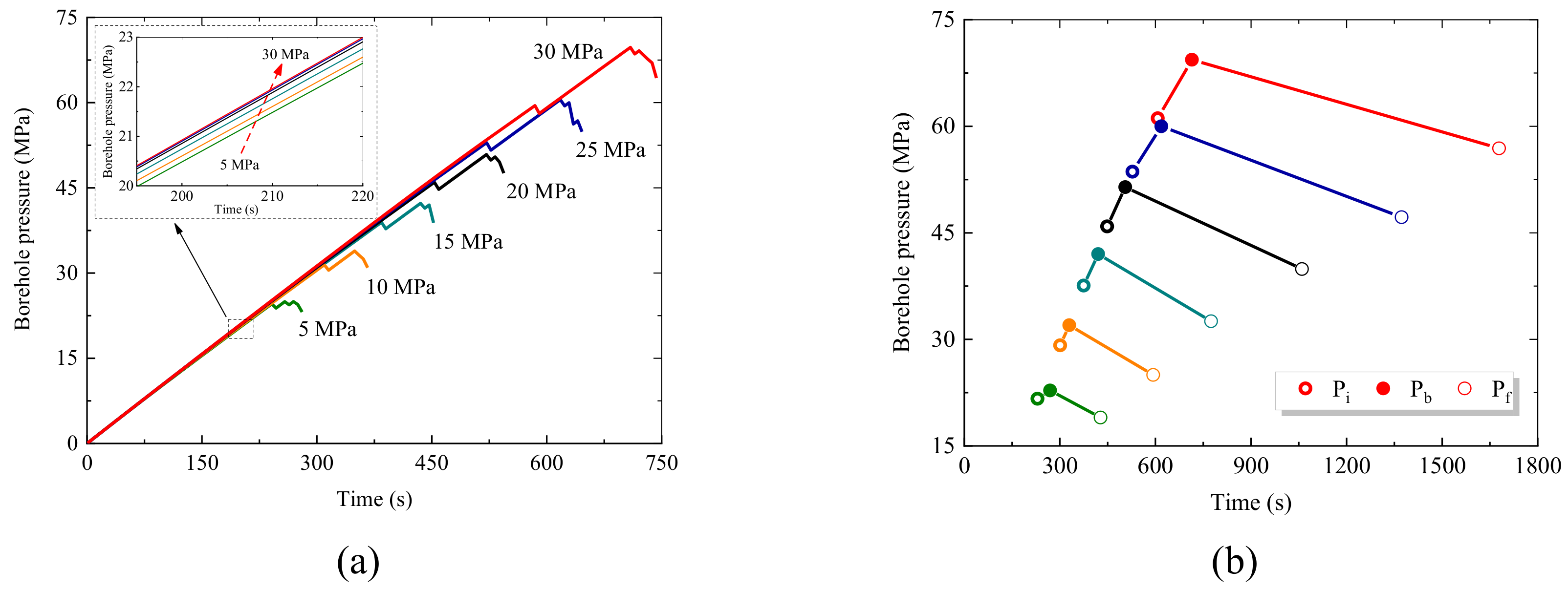
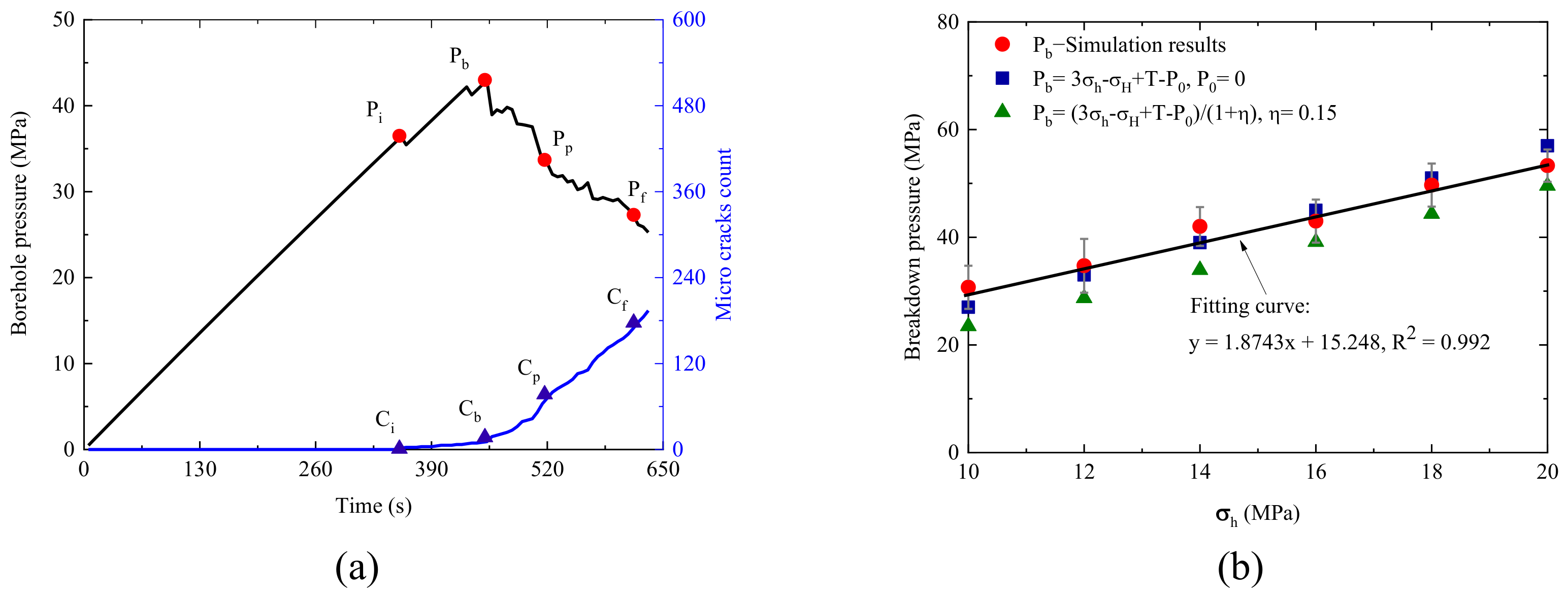
A set of typical curves of borehole pressure, as well as the micro-crack count, are first given in Figure 7a. It is clear that the curve of the borehole pressure presents three significant change stages: (1) fluid pressure increasing stage ($0-P_i$); (2) borehole breakage stage ($P_i-P_b$); (3) fracture propagation stage ($P_b-P_f$). Along with this process, one can also capture four key characteristic pressure points, including the initial cracking pressure $P_i$, breakdown pressure $P_b$, fracture propagation pressure $P_p$ and fracture though pressure $P_f$. This kind of borehole pressure variation is consistent with that observed in common laboratory tests.

In respect to breakdown pressure $P_b$, a classical equation ($P_b=3{\sigma }_h-{\sigma }_H+T-P_0$) is first proposed based on elasticity consideration to forecast breakdown pressure variation by assuming that the borehole fluid is not exchanged with the rock matrix [46,48]. However, in reality, the borehole fluid inherently communicates with the pore fluid and, subsequently, an improved equation ($P_b=\left(3{\sigma }_h-{\sigma }_H+T-P_0\right)/(1+\eta )$) is proposed [33,35]. With these theoretical solutions, further comparisons on breakdown pressure are provided in Figure 7. There is an acceptable difference between numerical results and theoretical solutions. Moreover, inspired by theoretical equations, the breakdown pressure can be regarded as a linear function of ${\sigma }_h$, ${\sigma }_H$, $P_0$ and T. This characteristic is also captured by the simulation results, as shown in Figure 7b. This introduced hydromechanical coupling model can well describe the variation in breakdown pressure with differential stress.

4. Parameter Sensitivity Analysis

After the assessment of hydromechanical coupling model, a series of numerical simulations are now conducted to investigate the influence of underlying factors on hydraulic fracturing behavior, such as in situ stress, differential stress, fluid injection rate, fluid viscosity, and borehole size.

In subsequent analysis, we will focus on the variation in borehole pressure and hydraulic fracturing propagation. To this end, the borehole pressure curves are also divided into three stages similar to that defined above. At the same time, to better compare hydraulic fracturing propagation, two additional representative simulated results are provided for each influencing factor.

4.1. Influence of In Situ Stress

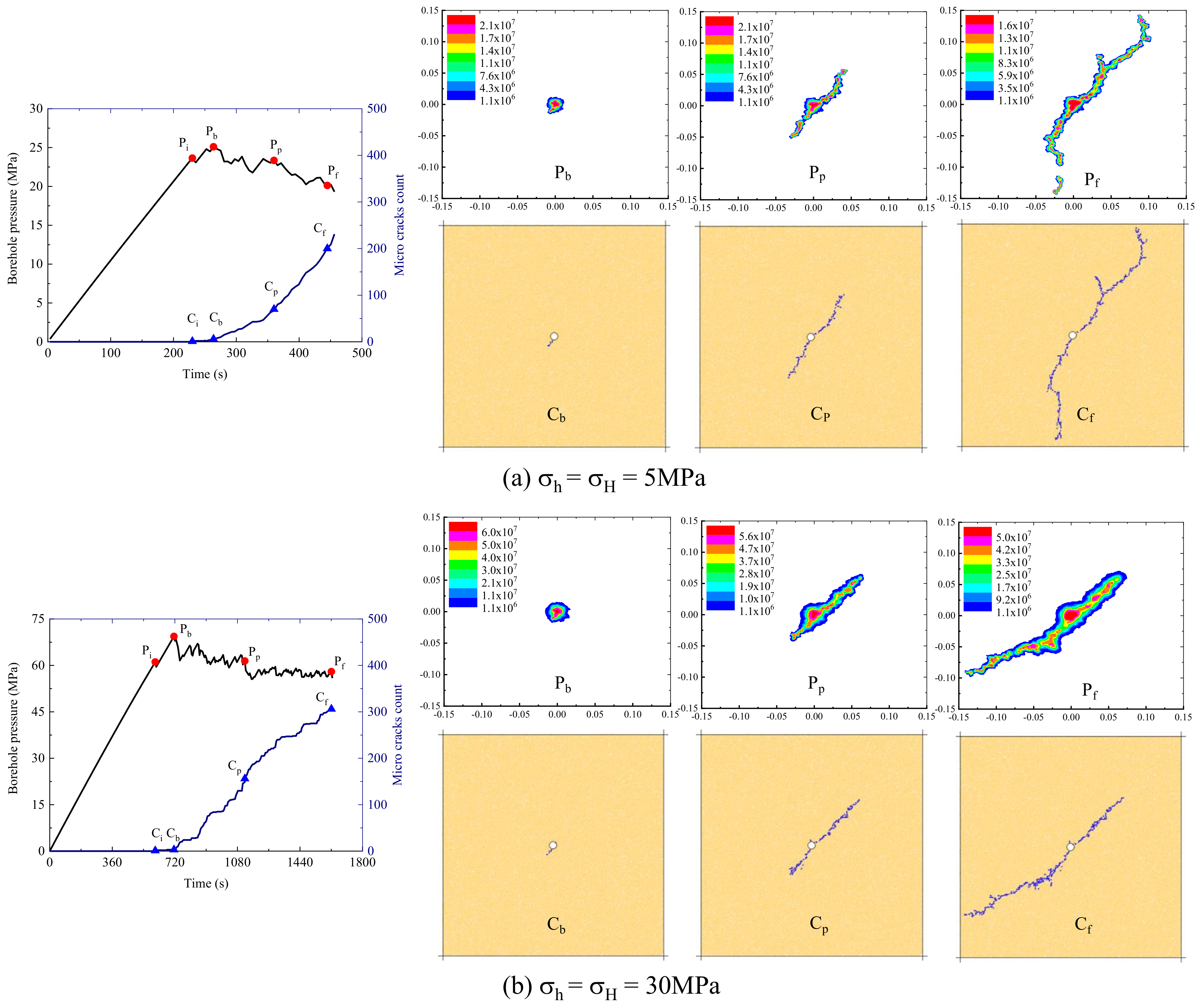
Conversely from other factors, in situ stress is an inherent property. Here, we first study the influence of this factor. For this purpose, a series of hydraulic fracturing simulations are conducted with confining stress (${\sigma }_h$, ${\sigma }_H$) increasing from 5 MPa to 30 MPa. Other micro parameters remain consistent as used above.

One can observe from Figure 8 that, with increasing confining pressure, the borehole pressure increase curve enhances and, correspondingly, the crack initiation pressure ($P_i$) and breakdown pressure ($P_b$) also increase. The increase in confining stress seems to be an advantage to borehole pressure. This trend is related to hydraulic aperture evolution. When confining stress increases, the hydraulic aperture reduces and thus leads to a decrease in permeability. For a borehole with the same injection fluid, the smaller the permeability is, the larger the increase in pressure. At the same time, due to a decrease in permeability, the duration of the fracture propagation also increases linearly.

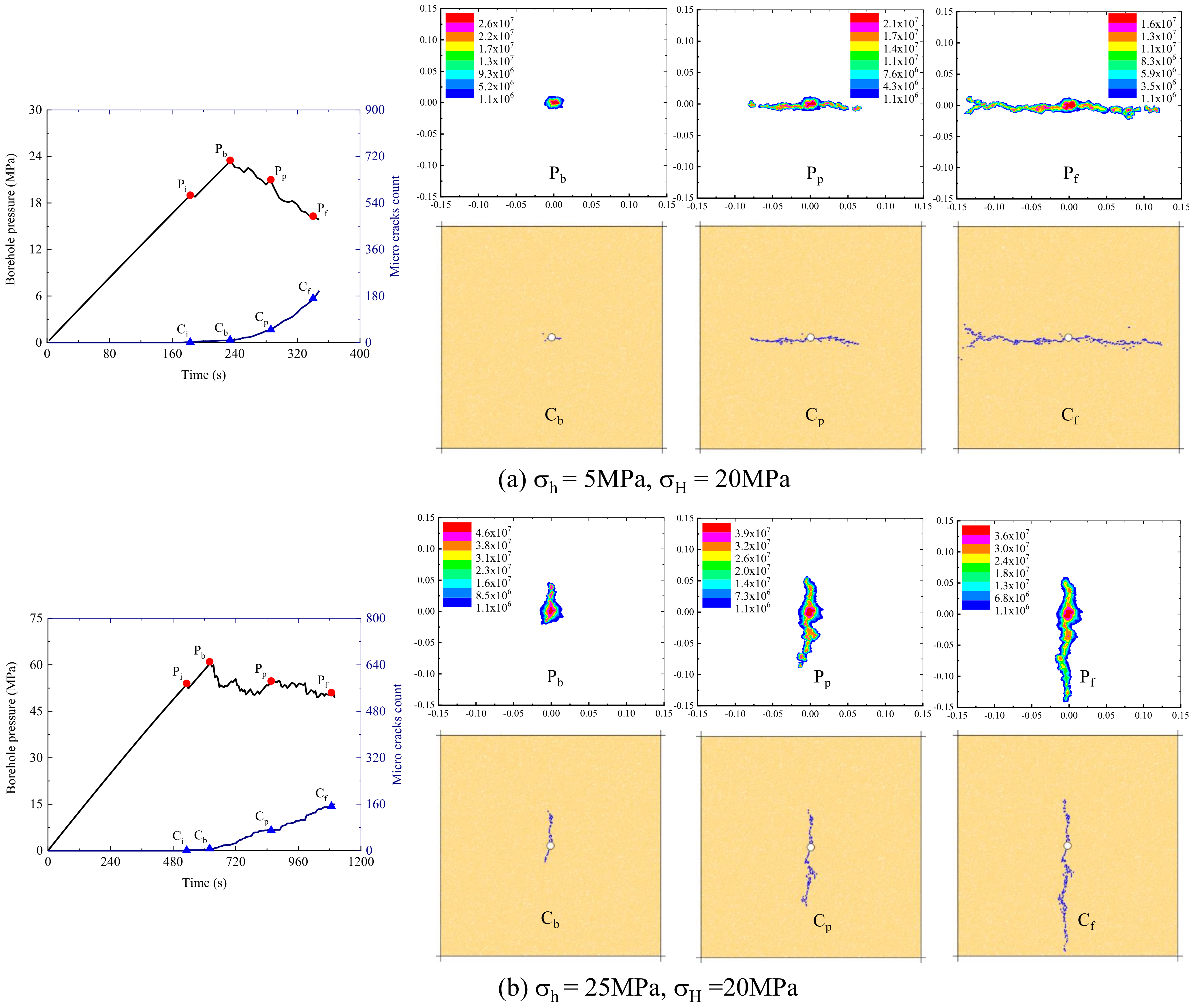
Two typical cases of 5 MPa and 30 MPa are further compared in Figure 9. According to the feature pressure of the borehole, the corresponding cracking states are provided. It is clear that under low confining stress, the cracking localization is sharp and forms one main fracture along with several branch-shaped cracks. This failure process presents obvious brittleness. For high confining stress limited by small permeability, the fracturing process is slow and thus leads to a smooth fracture formation. Hydraulic fracture propagation has typical ductile characteristics. Corresponding to this change, a concentrated fluid evolution band forms for low confining stress, and a diffusion zone for the large confining stress, such as shown in Figure 9.

4.2. Influence of Differential Stress

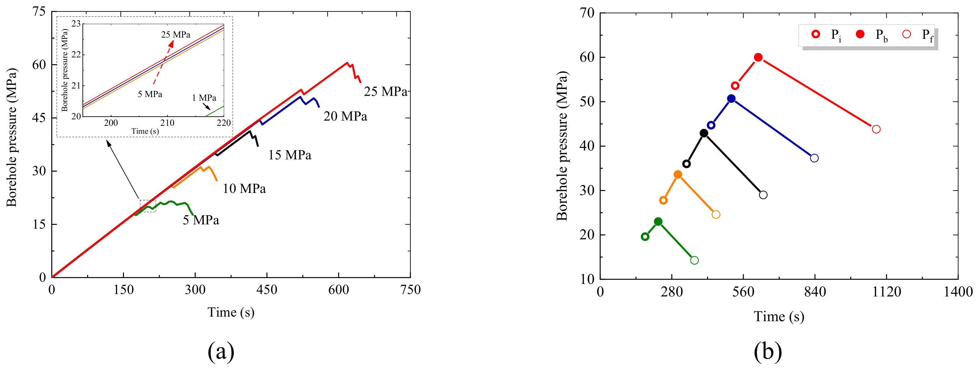
The influence of in situ stress difference is investigated in this section by maintaining ${\sigma }_H$ equal to 20 MPa and changing ${\sigma }_h$ to 5 MPa, 10 MPa, 15 MPa, 20 MPa and 25 MPa. Other micro parameters remain unchanged.

The variation curves of the borehole pressure, as well as time to fracture, are first given in Figure 10. It is clear that their change is similar to the case of hydrostatic stress. Increasing with minimum principal stress, the increase in the borehole pressure curve enhances and their corresponding feature pressure increases linearly. As for the time to fracture, we note the same linear increase that is often observed in laboratory tests [10,12].

Figure 11 shows hydraulic fracturing propagation in two representative cases. By contrast, their propagation has a large difference that changes from the horizontal direction to the vertical direction when the minimum principal stress increases from 5 MPa to 25 MPa. This change tendency is consistent with common experimental observation. Hydraulic fractures always propagate along the direction of maximum principal stress. In fact, hydraulic fracture propagation is essentially dependent on local stress evolution, which is directly related to in situ stress. The existence of differential in situ stress induces tensile force concentration. This feature drives hydraulic fracture propagation re-orientation. Therefore, the differential stress mainly affects the hydraulic fracturing direction. In addition, fluid pressure evolution along the fracture propagation is provided in Figure 11.

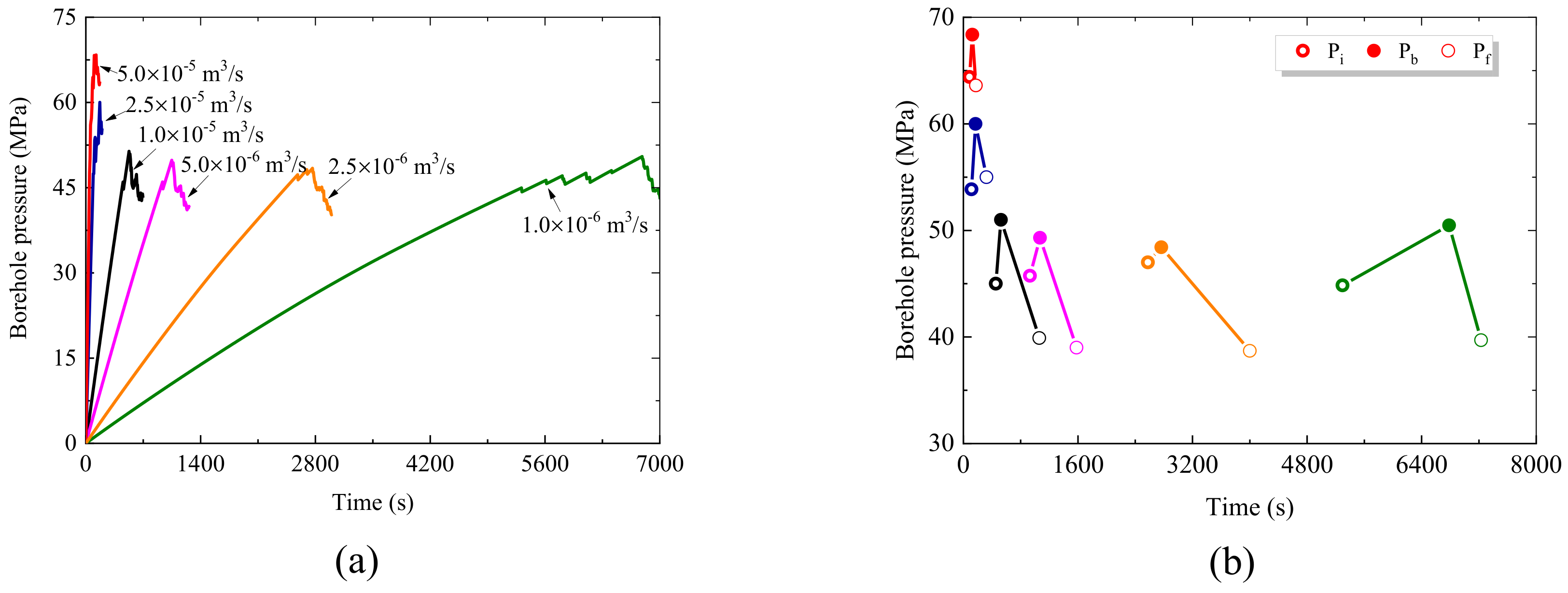
4.3. Influence of Fluid Injection Rate

In this section, keeping confining stress ${\sigma }_h$ and ${\sigma }_H$ as 20 MPa, the influence of the fluid injection rate on hydraulic fracturing behavior is investigated, with the injection rate changing from $1.0\times 10^{-6}$ m${}^3$/s, $2.5\times 10^{-6}$ m${}^3$/s, $5.0\times 10^{-6}$ m${}^3$/s, $1.0\times 10^{-5}$ m${}^3$/s, $2.5\times 10^{-5}$ m${}^3$/s, to $5.0\times 10^{-5}$ m${}^3$/s. Other parameters like mechanics, hydraulic parameters and fluid viscosity still remain constant.

Again, some representative curves are first given in Figure 12 in terms of borehole pressure and time to fracture. One can see that decreasing with fluid injection rate, the breakdown pressure first reduces sharply and then trends to a gentle value. At the same time, the increase in the borehole pressure curve becomes more and more non-linear, in particular at the injection rate of $1.0\times 10^{-6}$ m${}^3$/s. As for time to fracture, although the total time increase with fluid injection rate decreases, the prolonged time is mainly induced by the stage of $0-P_i$. Therefore, the change in fluid injection rate mainly influences the time before crack initiation.

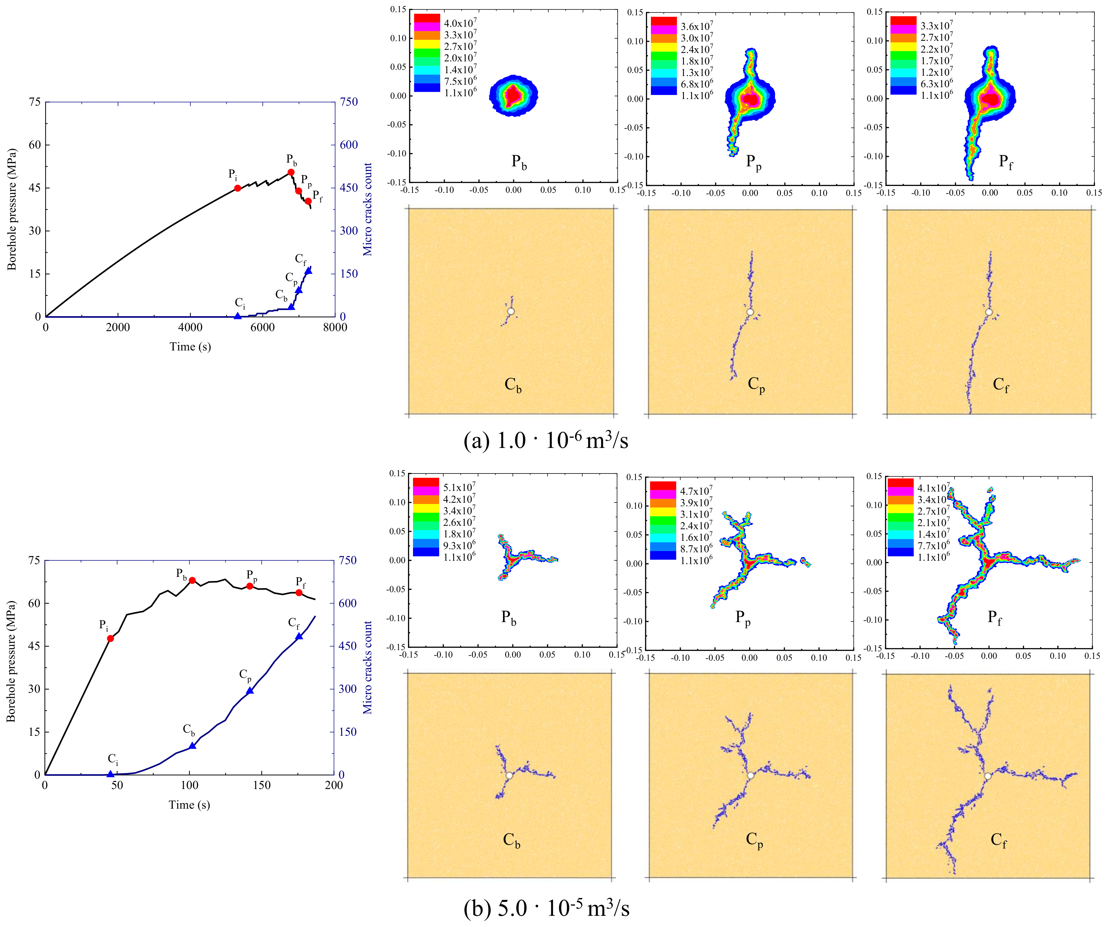
In addition, two typical cases with an injection rate of $1.0\times 10^{-6}$ m${}^3$/s and $5.0\times 10^{-5}$ m${}^3$/s are further compared in Figure 13. One can see that a relatively complex branch-shaped fracture is formed for a large rate of fluid injection, while a simple wing-shaped fracture is formed for a small one. It seems that the large injection rate can easily cause hydraulic fracture propagation. More precisely, the quickly increasing differential pressure of adjacent pores induced by a large fluid injection does not have enough time to diffuse, and thus leads to more crack formation. As a result, there is no distinct fluid diffusion band for the case of the large injection rate, but there is a clear fluid pressure evolution zone for the small one. More details can be found in Figure 13.

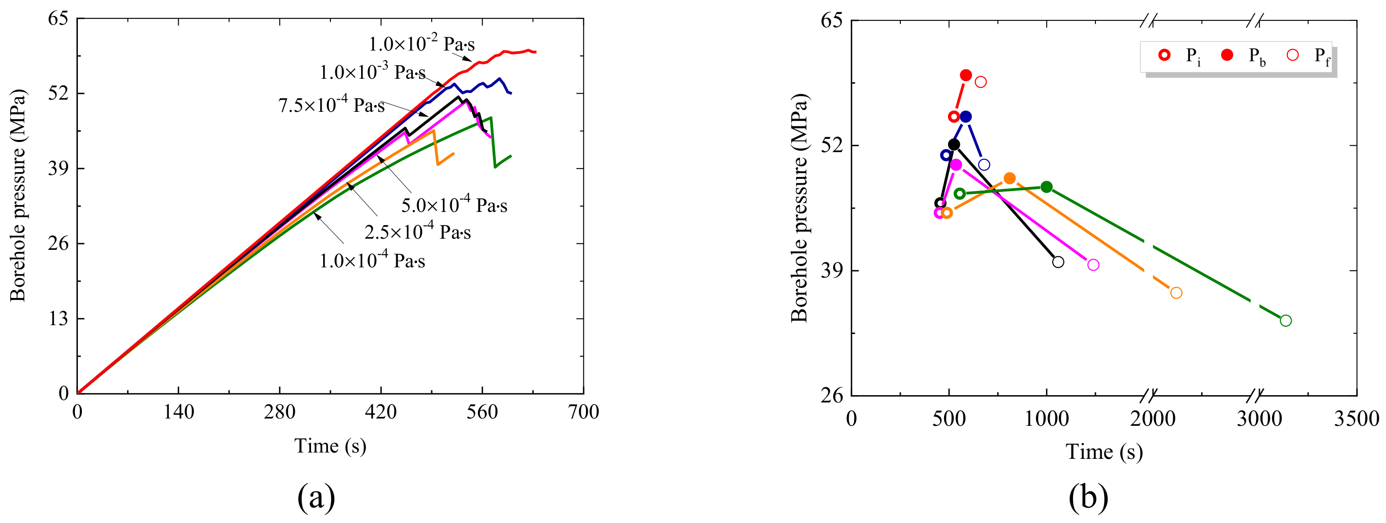
4.4. Influence of Fluid Viscosity

In order to assess the influence of fluid viscosity, a series of numerical hydraulic fracturing simulations are performed here by considering the different fluid viscosity of $1.0\times {10}^{-4}$ Pa · s, $2.5\times {10}^{-4}$ Pa · s, $5.0\times {10}^{-4}$ Pa · s, $7.5\times {10}^{-4}$ Pa · s, $1.0\times {10}^{-3}$ Pa · s and $1.0\times {10}^{-2}$ Pa · s. The injection rate is fixed to be $1.0\times 10^{-5}$ m${}^3$/s, and the in situ stress of both in the x and y direction remains constant at 20 MPa.

Results in Figure 14 show that with the decrease in fluid viscosity, the increasing degree of borehole pressure decline and the non-linear property of the corresponding curve becomes more significant. These pressure characteristics first drop quickly and then tend toward gentle values, especially breakdown pressure $P_i$. At the same time, the total time to fracture largely increases, and the prolonged part is focused on the stage of $P_i-P_f$. This change suggests that fluid viscosity mainly controls the time to fracture propagation.

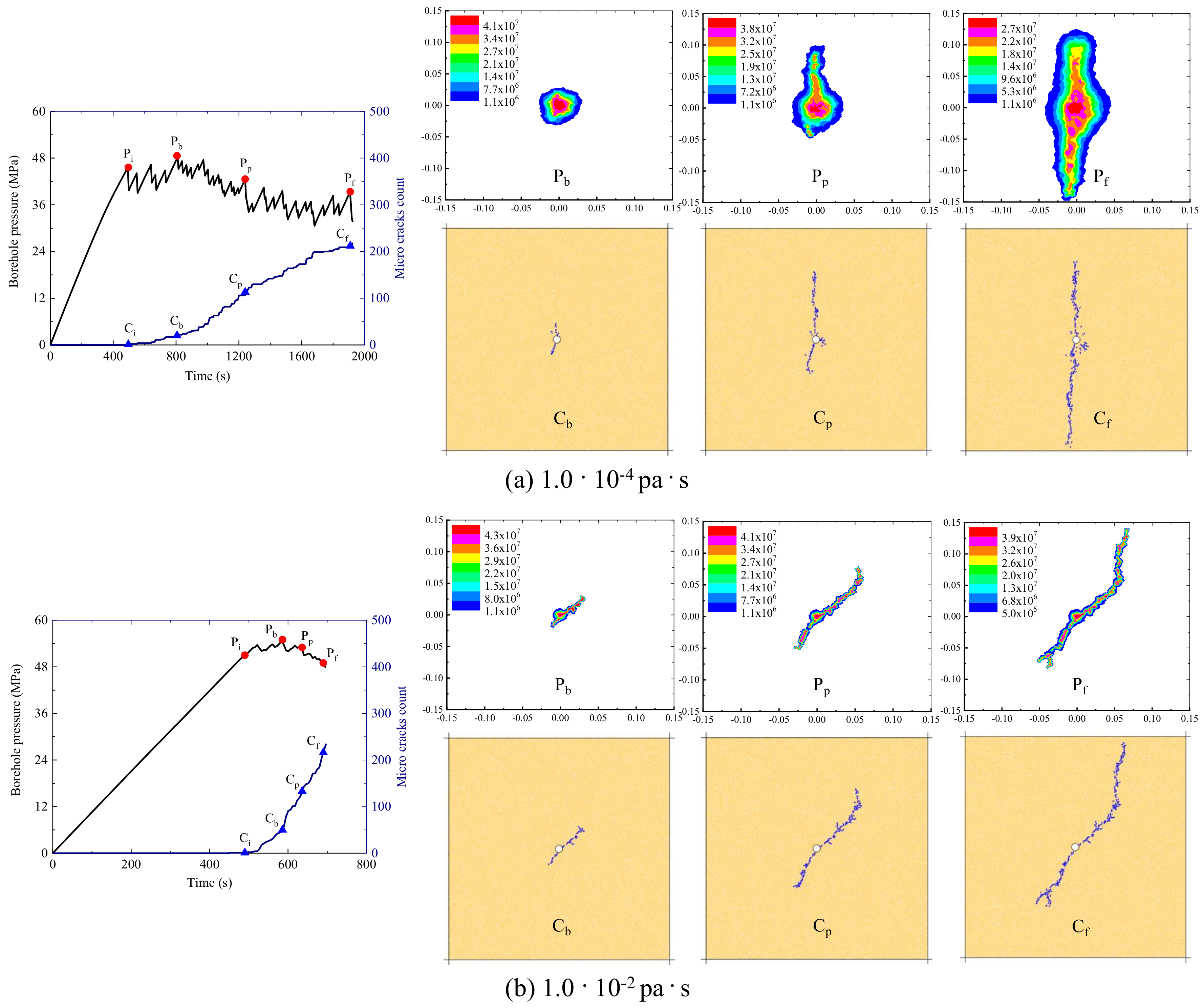
In this respect, two detailed comparisons of borehole pressure variation are provided in Figure 14a. Along with borehole pressure change, fluid pressure diffusion along fracture propagation also presents the corresponding evolution process. When fluid viscosity is low, the fluid has a relatively strong penetrating ability and thus one distinct distribution band with a clear pressure gradient forms around the borehole as well as along the fracture propagation. Whereas, when fluid viscosity is high, its flow ability declines, and the fluid pressure evolves mainly along the fracture propagation without diffusion into the rock matrix. As a consequence, a relatively complex fracture with branch-shaped cracks develops for a high viscosity fluid, but a simple one develops for a low viscosity fluid, as shown in Figure 15.

4.5. Influence of Borehole Radius

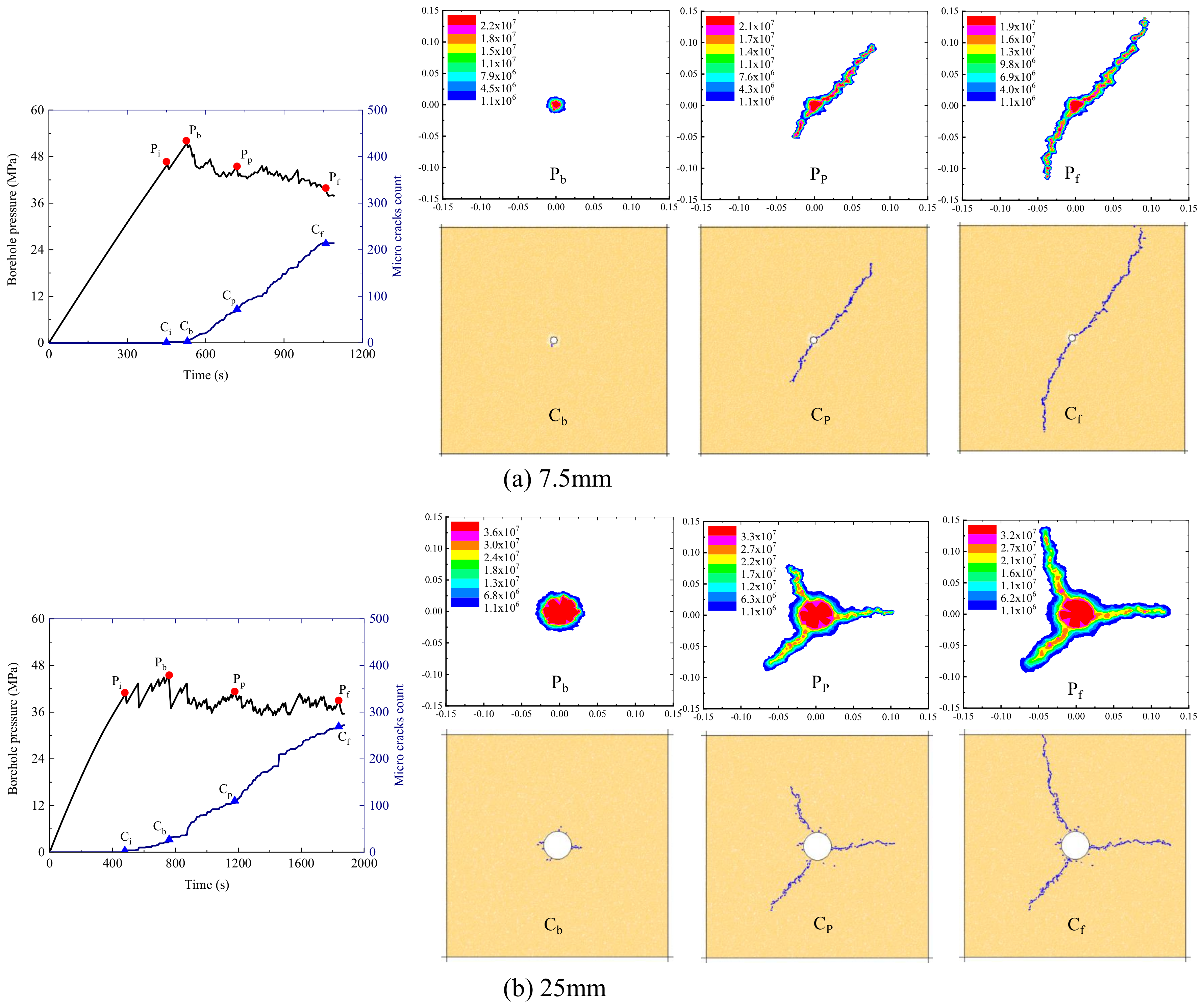
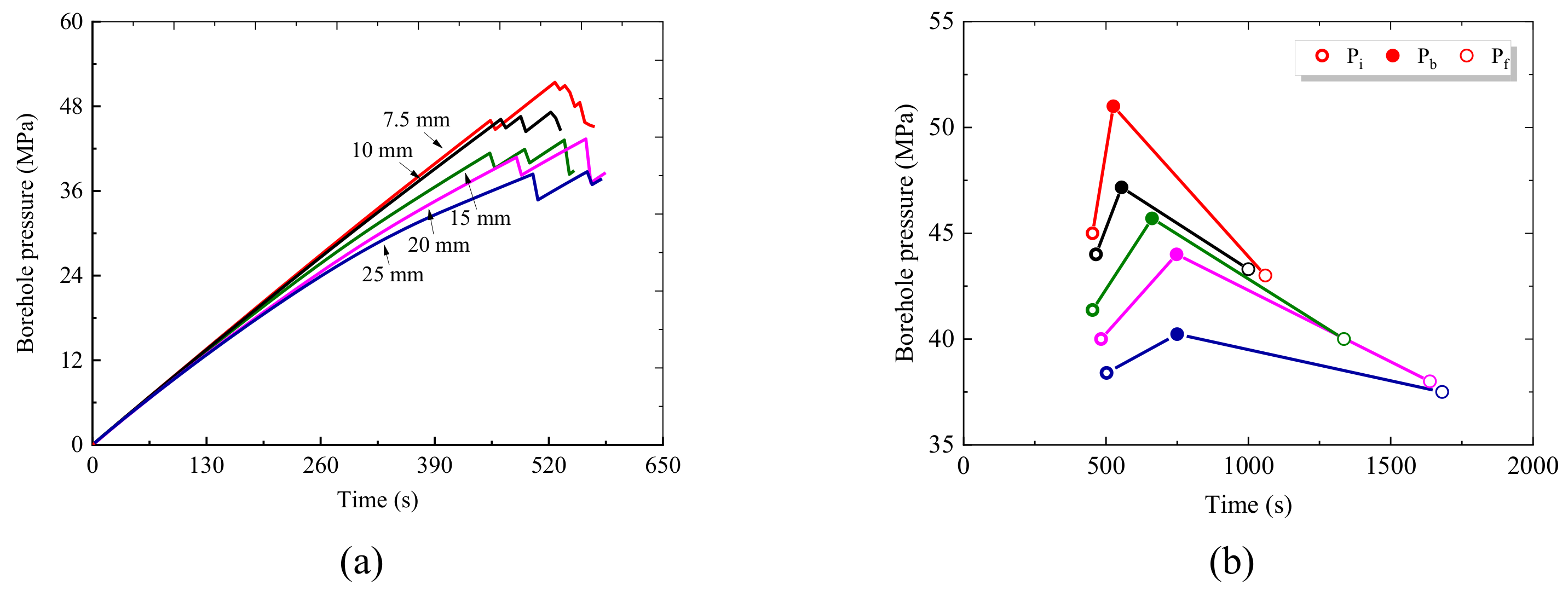
As one of the easily neglected factors, the effect of borehole radius on hydraulic fracturing behavior is investigated in this section, by conducting a series of numerical simulations with a sample radius changing from 7.5 mm, 10 mm, 15 mm, 20 mm to 25 mm. Other micro parameters remain the same as used above.

Figure 16 shows that as the borehole radius increases, the non-linear property of the pressure curves becomes more obvious, and the corresponding feature pressure gradually decreases. More interestingly, the differential value between breakdown pressure $P_b$ and fracture though pressure $P_f$ is also reduced, which further means that the increase in borehole radius seems to be a disadvantage for fluid injection pressurization. Consequently, the total time to fracture largely increases. In spite of that, the prolonged time is mainly concentrated at the stage of fracture propagation ($P_i-P_f$).

In addition, a detailed hydraulic fracture propagation, as well as fluid pressure evolution, are compared in Figure 17 for a borehole radius of 7.5 mm and 25 mm. It is clear that when the borehole radius is small, a symmetric wing-shaped fracture forms, along with a clear fluid pressure band. For the large borehole, three branch-shaped fractures develop around the borehole and accompany the relatively large fluid pressure evolution zone. The difference is due to the idea that the larger the fluid injection area is, the more underlying defects there are. As a result, this leads to hydraulic fracturing patterns becoming more complex.

5. Conclusions

In this paper, we have first introduced an improved hydraulic coupling model and then implemented it in the framework of particle flow simulation. This model can well describe variation in hydraulic aperture with normal contact force pre- and post contact bond breakage. Numerical parameter calibration and model assessment tests were then conducted. The introduced hydromechanical coupling model has the ability to describe local stress evolution around boreholes and fracture propagation outside of boreholes. With this model in hand, a series of parameter sensitive studies on hydraulic fracturing propagation have been performed, including in situ stress, differential stress, fluid injection rate, fluid viscosity and borehole size.

The obtained numerical results suggest that the increase either in hydrostatics stress or differential stress leads to borehole pressure linearly increasing, and the fracture pattern changing from brittle to ductile. Conversely, the variation in differential stress can induce hydraulic fracturing reorientation. The injection rate and fluid viscosity have a similar influence on hydraulic fracturing behavior where, as their values decrease, the non-linear increase in borehole pressure gradually becomes more obvious and the total time to fracture is substantially prolonged. However, the fluid injection rate mainly controls the time to the initial crack, while fluid viscosity decides the duration of the fracture propagation. The increase in borehole radius directly enhances the fluid diffusion zone, which further leads to injection pressure nonlinear property enhancement, a decrease in breakdown pressure, time to fracture prolongation, and hydraulic fracture complexity.

The inherent anisotropy of rocks should play an important role in the hydraulic fracturing process, and this feature will be investigated in our future studies.

References

- Damjanac, B.; Cundall, P. Application of distinct element methods to simulation of hydraulic fracturing in naturally fractured reservoirs. Comput. Geotech. 2016, 71, 283–294. [Google Scholar] [CrossRef]
- Warpinski, N.R.; Mayerhofer, M.J.; Vincent, M.C.; Cipolla, C.L.; Lolon, E.P. Stimulating Unconventional Reservoirs: Maximizing Network Growth While Optimizing Fracture Conductivity. J. Can. Pet. Technol. 2009, 48, 39–51. [Google Scholar] [CrossRef]
- Pruess, K. Enhanced geothermal systems (EGS) using CO2 as working fluid—A novel approach for generating renewable energy with simultaneous sequestration of carbon. Geothermics 2006, 35, 351–367. [Google Scholar] [CrossRef] [Green Version]
- Ilawe, N.V.; Zimmerman, J.A.; Wong, B.M. Breaking badly: DFT-D2 gives sizeable errors for tensile strengths in palladium-hydride solids. J. Chem. Theory Comput. 2015, 11, 5426–5435. [Google Scholar] [CrossRef] [PubMed]
- Lee, J.H.; Park, J.H.; Soon, A. Assessing the influence of van der Waals corrected exchange-correlation functionals on the anisotropic mechanical properties of coinage metals. Phys. Rev. B 2016, 94, 024108. [Google Scholar] [CrossRef] [Green Version]
- Goodfellow, S.D.; Nasseri, M.H.B.; Maxwell, S.C.; Young, R.P. Hydraulic Fracture Energy Budget: Insights From the Laboratory. Geophys. Res. Lett. 2015, 42, 3179–3187. [Google Scholar] [CrossRef]
- Zhou, J.; Jin, Y.; Chen, M. Experimental investigation of hydraulic fracturing in random naturally fractured blocks. Int. J. Rock Mech. Min. Sci. 2010, 47, 1193–1199. [Google Scholar] [CrossRef]
- He, J.; Afolagboye, L.O.; Lin, C.; Wan, X. An Experimental Investigation of Hydraulic Fracturing in Shale Considering Anisotropy and Using Freshwater and Supercritical CO2. Energies 2018, 11, 557. [Google Scholar] [CrossRef] [Green Version]
- Bohloli, B.; de Pater, C.J. Experimental study on hydraulic fracturing of soft rocks: Influence of fluid rheology and confining stress. J. Pet. Sci. Eng. 2006, 53, 1–12. [Google Scholar] [CrossRef]
- Sarmadivaleh, M.; Rasouli, V. Test design and sample preparation procedure for experimental investigation of hydraulic fracturing interaction modes. Rock Mech. Rock Eng. 2015, 48, 93–105. [Google Scholar] [CrossRef]
- Zhang, X.; Lu, Y.; Tang, J.; Zhou, Z.; Liao, Y. Experimental study on fracture initiation and propagation in shale using supercritical carbon dioxide fracturing. Fuel 2017, 190, 370–378. [Google Scholar] [CrossRef]
- Zhou, J.; Chen, M.; Jin, Y.; Zhang, G.Q. Analysis of fracture propagation behavior and fracture geometry using a tri-axial fracturing system in naturally fractured reservoirs. Int. J. Rock Mech. Min. Sci. 2008, 45, 1143–1152. [Google Scholar] [CrossRef]
- Aadnøy, B.S.; Belayneh, M. Elasto-plastic fracturing model for wellbore stability using non-penetrating fluids. J. Pet. Sci. Eng. 2004, 45, 179–192. [Google Scholar] [CrossRef]
- Haimson, B.C. The hydraulic fracturing method of stress measurement: Theory and practice. Rock Test. Site Charact. 1993, 67, 395–412. [Google Scholar]
- Hossain, M.M.; Rahman, M.K.; Rahman, S.S. Hydraulic fracture initiation and propagation: Roles of wellbore trajectory, perforation and stress regimes. J. Pet. Sci. Eng. 2000, 27, 129–149. [Google Scholar] [CrossRef]
- Huang, J.; Griffiths, D.V.; Wong, S.W. Initiation pressure, location and orientation of hydraulic fracture. Int. J. Rock Mech. Min. Sci. 2012, 49, 59–67. [Google Scholar] [CrossRef]
- Gan, Q.; Elsworth, D.; Alpern, J.; Marone, C.; Connolly, P. Breakdown pressures due to infiltration and exclusion in finite length boreholes. J. Pet. Sci. Eng. 2015, 127, 329–337. [Google Scholar] [CrossRef]
- Hamidi, F.; Mortazavi, A. A new three dimensional approach to numerically model hydraulic fracturing process. J. Pet. Sci. Eng. 2014, 124, 451–467. [Google Scholar] [CrossRef]
- Ma, X.; Zhou, T.; Zou, Y. Experimental and numerical study of hydraulic fracture geometry in shale formations with complex geologic conditions. J. Struct. Geol. 2017, 98, 53–66. [Google Scholar] [CrossRef]
- Nagel, N.B.; Sanchez-Nagel, M.A.; Zhang, F.; Garcia, X.; Lee, B. Coupled numerical evaluations of the geomechanical interactions between a hydraulic fracture stimulation and a natural fracture system in shale formations. Rock Mech. Rock Eng. 2013, 46, 581–609. [Google Scholar] [CrossRef]
- Nasehi, M.J.; Mortazavi, A. Effects of in-situ stress regime and intact rock strength parameters on the hydraulic fracturing. J. Pet. Sci. Eng. 2013, 108, 211–221. [Google Scholar] [CrossRef]
- Yushi, Z.; Xinfang, M.; Shicheng, Z.; Tong, Z.; Han, L. Numerical investigation into the influence of bedding plane on hydraulic fracture network propagation in shale formations. Rock Mech. Rock Eng. 2016, 49, 3597–3614. [Google Scholar] [CrossRef]
- Zhang, Y.; Liu, Z.; Shi, C.; Shao, J. Three-dimensional Reconstruction of Block Shape Irregularity and its Effects on Block Impacts Using an Energy-Based Approach. Rock Mech. Rock Eng. 2018, 51, 1173–1191. [Google Scholar] [CrossRef]
- Al-Busaidi, A.; Hazzard, J.F.; Young, R.P. Distinct element modeling of hydraulically fractured Lac du Bonnet granite. J. Geophys. Res. Solid Earth 2005, 110, B6. [Google Scholar] [CrossRef] [Green Version]
- Duan, K.; Kwok, C.Y. Evolution of stress-induced borehole breakout in inherently anisotropic rock: Insights from discrete element modeling. J. Geophys. Res. Solid Earth 2016, 121, 2361–2381. [Google Scholar] [CrossRef] [Green Version]
- Reinicke, A.; Rybacki, E.; Stanchits, S.; Huenges, E.; Dresen, G. Hydraulic fracturing stimulation techniques and formation damage mechanisms—Implications from laboratory testing of tight sandstone–proppant systems. Chem. Der-Erde-Geochem. 2010, 70, 107–117. [Google Scholar] [CrossRef]
- Zhang, Y.; Han, B.; Zhang, X.; Jia, Y.; Zhu, C. Study of Interactions between Induced and Natural Fracture Effects on Hydraulic Fracture Propagation Using a Discrete Approach. Lithosphere 2021, Special 4, 5810181. [Google Scholar] [CrossRef]
- Hazzard, J.F.; Young, R.P.; Oates, S.J. Numerical modeling of seismicity induced by fluid injection in naturally fractured reservoir. Geophysics 2011, 76, WC167–WC180. [Google Scholar]
- Eshiet, K.I.; Sheng, Y.; Ye, J. Microscopic modelling of the hydraulic fracturing process. Environ. Earth Sci. 2013, 68, 1169–1186. [Google Scholar] [CrossRef]
- Fatahi, H.; Hossain, M.M.; Sarmadivaleh, M. Numerical and experimental investigation of the interaction of natural and propagated hydraulic fracture. J. Nat. Gas Sci. Eng. 2017, 37, 409–424. [Google Scholar] [CrossRef] [Green Version]
- Hazzard, J.F.; Young, R.P.; Oates, S.J. Numerical modeling of seismicity induced by fluid injection in a fractured reservoir. In Mining and Tunnel Innovation and Opportunity, Proceedings of the 5th North American Rock Mechanics Symposium, University of Toronto Press, Toronto, ON, Canada, 7–10 July 2002; University of Toronto Press: Toronto, ON, Canada, 2002; Volume 32, pp. 1023–1030. [Google Scholar]
- Wang, T.; Hu, W.; Elsworth, D.; Zhou, W.; Zhou, W.; Zhao, X.; Zhao, L. The effect of natural fractures on hydraulic fracturing propagation in coal seams. J. Pet. Sci. Eng. 2017, 150, 180–190. [Google Scholar] [CrossRef]
- Wang, T.; Zhou, W.; Chen, J.; Xiao, X.; Li, Y.; Zhao, X. Simulation of hydraulic fracturing using particle flow method and application in a coal mine. Int. J. Coal Geol. 2014, 121, 1–13. [Google Scholar] [CrossRef]
- Zhang, Y.; Shao, J.; Liu, Z.; Shi, C. An improved hydromechanical model for particle flow simulation of fractures in saturated rocks. Int. J. Rock Mech. Min. Sci. 2021, 147, 104870. [Google Scholar] [CrossRef]
- Duan, K.; Kwok, C.Y.; Wu, W.; Jing, L. DEM modeling of hydraulic fracturing in permeable rock: Influence of viscosity, injection rate and in situ states. Acta Geotech. 2018, 13, 1187–1202. [Google Scholar] [CrossRef]
- Shimizu, H.; Murata, S.; Ishida, T. The distinct element analysis for hydraulic fracturing in hard rock considering fluid viscosity and particle size distribution. Int. J. Rock Mech. Min. Sci. 2011, 48, 712–727. [Google Scholar] [CrossRef]
- Zhang, Q.; Zhang, X.P.; Ji, P.Q.; Zhang, H.; Tang, X.; Wu, Z. Study of interaction mechanisms between multiple parallel weak planes and hydraulic fracture using the bonded-particle model based on moment tensors. J. Nat. Gas Ence Eng. 2020, 76, 103176. [Google Scholar] [CrossRef]
- Cundall, P.A. PFC2D User’s Manual (Version 3.1); Itasca Consulting Group Inc.: Minneapolis, MN, USA, 2004; Volume 325. [Google Scholar]
- Cundall, P.A. PFC2D User’s Manual (Version 4.0); Itasca Consulting Group Inc.: Minneapolis, MN, USA, 2008; Volume 237. [Google Scholar]
- Potyondy, D.O.; Cundall, P.A. A bonded-particle model for rock. Int. J. Rock Mech. Min. Sci. 2004, 41, 1329–1364. [Google Scholar] [CrossRef]
- Zhang, Y.; Shao, J.; Liu, Z.; Shi, C.; De Saxcé, G. Effects of confining pressure and loading path on deformation and strength of cohesive granular materials: A three-dimensional DEM analysis. Acta Geotech. 2019, 14, 443–460. [Google Scholar] [CrossRef]
- Zhang, Y.; Shao, J.; de Saxcé, G.; Shi, C.; Liu, Z. Study of deformation and failure in an anisotropic rock with a three-dimensional discrete element model. Int. J. Rock Mech. Min. Sci. 2019, 120, 17–28. [Google Scholar] [CrossRef]
- Zhang, Y.; Liu, Z.; Han, B.; Zhu, S.; Zhang, X. Numerical study of hydraulic fracture propagation in inherently laminated rocks accounting for bedding plane properties. J. Pet. Sci. Eng. 2022, 210, 109798. [Google Scholar] [CrossRef]
- Zhou, J.; Zhang, L.; Han, Z. Hydraulic fracturing process by using a modified two-dimensional particle flow code-method and validation. Prog. Comput. Fluid Dyn. Int. J. 2017, 17, 52–62. [Google Scholar] [CrossRef]
- Zhou, J.; Zhang, L.; Pan, Z.; Han, Z. Numerical investigation of fluid-driven near-borehole fracture propagation in laminated reservoir rock using PFC 2D. J. Nat. Gas Sci. Eng. 2016, 36, 719–733. [Google Scholar] [CrossRef]
- Haimson, B.C.; Cornet, F.H. ISRM suggested methods for rock stress estimation—Part 3: Hydraulic fracturing (HF) and/or hydraulic testing of pre-existing fractures (HTPF). Int. J. Rock Mech. Min. Sci. 2003, 40, 1011–1020. [Google Scholar] [CrossRef]
- Haimson, B. Micromechanisms of borehole instability leading to breakouts in rocks. Int. J. Rock Mech. Min. Sci. 2007, 44, 157–173. [Google Scholar] [CrossRef]
- Fairhurst, C. Stress estimation in rock: A brief history and review. Int. J. Rock Mech. Min. Sci. 2003, 40, 957–973. [Google Scholar] [CrossRef]
Figure 1.
Illustration of numerical rock sample: (a) Particle–based numerical model; (b) Particle–particle bonded contact; (c) Particle–boundary contact.
Figure 2.
Basic mechanical behavior at contacts: (
a) Normal force versus normal displacement; (
b) Shear force versus shear displacement; (
c) Peak and residual strength envelopes of nonlinear failure criterion for bond contact [
41].
Figure 3.
Fluid network model and implemented mechanism: (a) Solid particles (yellow circles), flow channels (blue lines), domains (red polygons) and domain centers (blue points); (b) Calculation of fluid flow in domain and pipe; (c) Fluid pressure evolution post bond breakage.
Figure 4.
Implementation of fluid flow simulation (a) boundary setting and (b) corresponding simulated results.
Figure 5.
Generation of numerical sample and setting of measurement circles for hydraulic fracturing simulation.
Figure 6.
Comparisons of local stresses obtained theoretically and numerically: (a) Around borehole; (b) Along x direction.
Figure 7.
Results of hydraulic fracturing simulation: (a) Representative curves of borehole pressure and micro cracks ( = 20 MPa, = 15 MPa); (b) Comparison of numerical prediction and theoretical solution.
Figure 8.
Effect of hydrostatic stress values on hydraulic fracturing behavior with respect to (a) borehole pressure response and (b) time to fracture.
Figure 9.
Comparisons of hydraulic fracturing behaviors in terms of borehole pressure (MPa), fluid pressure (Pa) distribution and crack propagation for two representative hydrostatic stress values.
Figure 10.
Effect of differential stress on hydraulic fracturing behavior in respect of (a) borehole pressure response and (b) time to fracture.
Figure 11.
Comparisons of hydraulic fracturing behaviors in terms of borehole pressure (MPa), fluid pressure (Pa) distribution and crack propagation for two representative differential stress values.
Figure 12.
Effect of fluid injection rate on hydraulic fracturing behavior in respect of (a) borehole pressure response and (b) time to fracture.
Figure 13.
Comparisons of hydraulic fracturing behaviors in terms of borehole pressure (MPa), fluid pressure (Pa) distribution and crack propagation for two representative fluid injection rates.
Figure 14.
Effect of fluid viscosity on hydraulic fracturing behavior in respect of (a) borehole pressure response and (b) time to fracture.
Figure 15.
Comparisons of hydraulic fracturing behaviors in terms of borehole pressure (MPa), fluid pressure (Pa) distribution and crack propagation for two representative fluid viscosity values.
Figure 16.
Effect of borehole radius on hydraulic fracturing behavior with respect to (a) borehole pressure response and (b) time to fracture.
Figure 17.
Comparisons of hydraulic fracturing behaviors in terms of borehole pressure (MPa), fluid pressure (Pa) distribution and crack propagation for two representative borehole radius values.