Article

Diagnostic Column Reasoning Based on Multi-Valued Evaluation of Residuals and the Elementary Symptoms Sequence

Institute of Automatic Control and Robotics, Warsaw University of Technology, Boboli 8, 02-525 Warsaw, Poland
*
Author to whom correspondence should be addressed.
These authors contributed equally to this work.
Energies 2022, 15(7), 2614; https://doi.org/10.3390/en15072614
Submission received: 2 February 2022 / Revised: 21 March 2022 / Accepted: 29 March 2022 / Published: 3 April 2022

Abstract

:
The paper concerns a significant problem in the diagnostics of industrial processes, which is the need to achieve high fault distinguishability. High distinguishability results in the generation of precise diagnoses that enable making appropriate security decisions. In the known approaches, the efforts to obtain high distinguishability are focused on the selection of an appropriate set of generated residuals. The paper presents a new method of diagnostic reasoning using the notation of faults/diagnostic signals’ relations in the form of a Fault Isolation System (FIS), which enables the use of multivalent diagnostic signals. In addition, the proposed method uses knowledge (usually incomplete) about the sequence of symptoms. Reasoning was carried out on the basis of simple, physically possible signatures, resulting from the FIS. Assumptions and a diagnostic algorithm are given. The reasoning algorithm works in a step-by-step manner, after observing further symptoms. In each reasoning step, two diagnoses are generated in parallel. A more accurate, but less certain diagnosis is formulated on the basis of the value of all diagnostic signals, and the diagnosis is less accurate, but more reliable, solely on the basis of symptoms. An example of using the method for diagnosing a set of connected liquid tanks is given. The method was compared with other reasoning methods based on columns (signatures) and, also, with row-based reasoning methods. It is shown that the proposed method allows the increase of the distinguishability of faults compared to other methods. The distinguishability grows with the knowledge of elementary symptom sequences. It is also noted that the proposed approach makes possible diagnosing not only faults, but also cyber attacks.

1. Introduction

The importance of model-based automatic fault diagnosis is growing steadily in industrial control systems. This is due to the disadvantages of commonly used alarm systems, which are the simplest diagnostic systems, as well as the advantages of advanced diagnostics, which contribute to increasing the efficiency and safety of processes. In the case of critical facilities, a properly functioning diagnostic system may prevent accidents that may threaten human health or life, as well as the natural environment.
Fault detection is carried out using a variety of models: analytical [1,2], neural [3,4], fuzzy [5,6], and statistical [7]. Only if the analytical models that take into account the impact of a fault on the residuals are known [2] is it possible to determine the relationship between the residuals and the faults. This relationship is necessary for fault isolation. In practice, models that represent the process state without any fault are usually used. In such cases, there are two options for obtaining knowledge about the impact of faults on residuals: using expert knowledge [1] or learning [8]. The learning technique requires the acquisition of experimental data not only for the normal state, but also for all faulty states that are to be recognised. In practice, this is impossible, because some faults are very rare, and the diagnostic system should recognise their first occurrence. Therefore, classification methods that require training data can only be used in special cases. The fault isolation methods that use expert knowledge to design the relationship between diagnostic signals resulting from the assessment of residuals and faults are of fundamental importance.
The simplest form of this relationship is the Fault Signature Matrix (FSM) [9,10,11], in which rows represent binary diagnostic signals and columns correspond to faults. A signature is a set of diagnostic signal values corresponding to a given fault. This form of notation of the fault–symptom relationship is also referred to as: the effect of the faults on the residuals [12] or a binary diagnostic matrix [13]. Another way to write the fault–diagnostic signal relation is the Fault Isolation System (FIS) [13,14], in which multivalued diagnostic signals are allowed.
In model-based diagnostics and FSM or FIS, two different approaches to diagnostic reasoning can be distinguished: column reasoning and row reasoning. In this classification, the columns or rows refer to the tabular record of the relationship, the knowledge of which is necessary to isolate faults.
Column-based (also known as signature-based) reasoning is commonly used in the FDI approach, while all diagnostic algorithms developed in a DX group, derived from the Reiter theory [15], represent row-based reasoning. Other works are also known, in which reasoning based on rows was used differently from the Reiter-based approach, e.g., [16].
All other forms of notation of the relationship between binary or multivalued diagnostic signals and faults are derived from FSM or FIS notations. Both IF–THEN rules, as well as logical functions or fault trees can be derived from the FSM or FIS [17].
In order to achieve a high distinguishability of faults, it is appropriate to use multivalued diagnostic signals instead of binary signals [17,18,19]. In model-based diagnostics, this usually means taking into account the residual sign, i.e., the use of a three-value residual evaluation.
In most diagnostic algorithms, only diagnostic signal values are used. However, as shown in many works (e.g., [10,20,21]), it is appropriate to take into account the knowledge about delays in the formation of symptoms. This can protect against false diagnoses in the period before all the symptoms of the fault are revealed. However, such knowledge can be also used to increase the distinguishability of faults. High differentiation leads to precise diagnosis, which results in making the right decisions to secure the process. These decisions can be made automatically as in Fault-Tolerant Control (FTC) systems or by process operators.
The contribution of the article consists of presenting a proposal for a new method of diagnostic reasoning based on three-value fault signatures with the use of knowledge about the sequence of symptoms, which may be incomplete. The aim of taking into account the knowledge of the residual signs and the known symptom sequences was to obtain a high distinguishability of faults. An additional contribution of this work is conducting a comparative analysis of the new approach with other known methods of inference.
The new reasoning algorithm uses a three-value residual evaluation and the knowledge of the sequence in which symptoms appear in the form of elementary sequences of symptoms proposed in [16]. There may appear temporary false diagnoses before all the symptoms of the fault are revealed in the case of column-based reasoning. Two parallel procedures are used in the new algorithm to achieve a proper diagnosis at any time of reasoning. One of them determines diagnoses based on all the values of the diagnostic signals, while the other utilises only observed symptoms.
An alternative reasoning algorithm was presented in [5]. The method also uses the FIS and knowledge of elementary symptom sequences, but the reasoning is based on rows. The methods of reasoning based on rows and columns differ in operational properties. Row-based reasoning eliminates false diagnoses resulting from delays in symptoms forming, but at the cost of less precise diagnosis in relation to column-based reasoning.
This paper focuses on the analysis of reasoning methods based on columns. The same process and the same set of models were used for the generation of residuals in a considered example. The aim was to calculate and compare the diagnostic quality indicators for all analysed algorithms. Using the results of the work [1], the accuracy of diagnosing for both groups of diagnostic reasoning methods was compared.
The structure of the work is as follows: Section 2 contain the review of known methods of fault detection and isolation. Section 3 discusses the differences between column-based and row-based reasoning. Section 4 introduces a new inference algorithm based on the fault isolation system and the sequence of symptoms. Section 5 presents the example application of the proposed algorithm for a set of serially connected buffer tanks.

2. The Knowledge and Data Used to Isolate Faults

To be able to carry out diagnostic reasoning, it is necessary to have specific knowledge of the diagnosed process and up-to-date data on the results of fault detection. The more accurate the knowledge and the corresponding collection of data, the higher the quality of the diagnoses generated is [10].
The most complete description of the process being diagnosed is a nonlinear analytical model that takes into account the impact of the inputs, as well as faults on the process outputs. Such models contain the knowledge needed not only for the detection, but also for the isolation of faults. In the case of a linear model, structural, directional, or sequential [17] computational and internal form residuals can be obtained. However, acquiring such models, especially for non-linear problems, is very difficult and, sometimes, even impossible.
This work considers a typical case for complex processes, in which only models representing the state of the process without faults are known. Therefore, we assumed that the quantitative knowledge of the sensitivity of residuals to faults is unknown. The relationship between the values of diagnostic signals, resulting from the evaluation of residuals, and faults was determined on the basis of expert knowledge. In this case, it has a qualitative nature, and it takes into account the sensitivity of the residuals to the faults in a binary manner (FSM case) or, additionally, the sign of the residual is also considered (FIS case).
In addition, heuristic knowledge of the time dependences of symptoms’ formation can also be used in diagnostic reasoning. The unequal times of various symptoms forming of the same fault pose a problem of reasoning that takes into account, not only the symptoms, but also zero values of diagnostic signals. This mainly applies to column-based reasoning, but also to row-based reasoning methods, in which the exonerationassumption is made. An example is the DTS method [22]. The problem disappears in the DX approach [15,23] and reasoning algorithms based only on symptoms [24], in which the above assumption is rejected.
The problem of delays in the appearance of symptoms was analysed in [10,16,20,24,25,26,27]. There are several methods of protecting the fault isolation algorithm against generating false diagnoses due to the delays of symptoms forming. Minimal and maximal delay times of symptoms of a given fault were used in [27], which allowed for a higher distinguishability of faults. However, estimating the minimum and maximum delay times for symptoms is very difficult. Defining the delay of a symptom by specifying a fuzzy time frame in the form of a trapezoid membership function, proposed in [10], is a similar solution.
In [16], the FSM and heuristic knowledge (usually incomplete) about the order in which the symptoms were observed were used to carry out row-based reasoning without the exonerationassumption. The development of this approach is the diagnostic reasoning method presented in [5].
The fault isolation algorithm can also be improved by considering the size of the residuals (large threshold violation or only a small signal activation) and the residuals’ sensitivity with respect to a certain fault [10]. However, at the design stage, the acquisition of such data is related to the knowledge of the residuals in an internal form, dependent on faults. At the outset, however, it was assumed that quantitative knowledge of the sensitivity of the residuals to faults is not known. The elements of knowledge regarding the diagnosed object and the data used in the proposed diagnostic reasoning algorithm are defined below.

2.1. Symptoms–Process Variables Relationship

The set of all Z variables used for fault detection includes control signals U and measurement signals Y.
Z = U Y = { z i : i = 1 , 2 , , I }
Residuals are either calculated as the difference between the modelled value and the measured one or between the left and right side of the equation describing the controlled part of the process [13]. The latter case concerns analytical models whose form is entangled with the output signal. For the isolation of a fault, a set of R residuals is used:
R = r j : j = 1 , 2 , , J
During the DS operation, residual values are calculated. As a result of the evaluation of residual values r j R , diagnostic signals s j S are formed, whereby:
S = s j : j = 1 , 2 , , J
One can define the relationship R S Z on the Cartesian product of the S and Z sets:
R S Z S × Z
The expression s j , z i R S Z means that the value of the process variable z i is used by the jth test to generate the diagnostic signal s j .
One can define a bidirectional graph G S Z :
G S Z = S , Z , R S Z
whose set of vertices consists of sets of diagnostic signals S and process variables Z. The set of the graph edges is described by the relation R S Z . This graph defines the sets of process variables used for the generation of particular diagnostic signals.

2.2. Symptoms–Faults Relation

There are two basic forms of notation for qualitative knowledge of the relationship between diagnostic signal values and faults, which can be designed based on expert knowledge. These are the F S M and F I S . By using the F S M , as well as the F I S , one can specify reasoning algorithms based on both columns and rows. The difference between these solutions is that: in the case of the F S M , binary diagnostic signals are taken into account, while in the case of the F I S , multivalued signals are used. An F S M example is shown in Table 1, while Table 2 shows an example of the F I S .
To describe the relationship between symptoms and faults when using binary residual evaluation, the F S M is used. When using the three-value evaluation of residuals 0 , + 1 , 1 , the F I S is used. This notation allows the use of model-based diagnostic signals, as well as the ones generated with the use of other techniques, e.g., from video sensors.
The F S M is a special case of the F I S . In order to introduce the concepts necessary for further consideration, a formal description of the F I S is given, as introduced in the work [13,14].
The F I S is defined as follows:
F I S = F , S , V S , q
where F is a finite set of faults,
F = f k : k = 1 , 2 , , K
S is a finite set of diagnostic signals determined by a dependency (3), and V S is a set of all diagnostic signal values:
V S = s j S V j
The q function specified on the Cartesian product F × S :
q : F × S Φ V S
and assigns to each pair of fault and diagnostic signals s j , f k a subset of diagnostic signal values, which can observe when f k fault occurs:
q s j , f k V j k = ν j i k V j , V j
Therefore, F I S is an array that specifies the diagnostic signal reference values for each fault. If the set of values for all diagnostic signals is the same and equals V S = 0 , 1 , then the F I S is simplified to the F S M .
The fault signature corresponds to the F I S column and is determined by the dependency:
Q f k = [ V 1 k , , V j k , , V J k ] T
The examples given in Table 1 and Table 2 illustrate the differences between the F S M and F I S . They are as follows:
  • In the F S M , each diagnostic signal s j can take only one of two values V j = { 0 , 1 } , while in the F I S , the set V j can be multivalued and each diagnostic signal s j can have its own individual set of values V j (zero always means no symptom);
  • Each table item contains only one value, while any table item in F S M s j , f k can contain a subset of values V j k V j ;
  • The fault signatures corresponding to the table columns (Table 1) in the F S M case contain only single signal values (simple signatures), while in the F I S case (Table 3), they can also contain subsets of the values of each diagnostic signal (complex signatures). Each complex signature can be replaced with a set of simple signatures, as illustrated in Table 3. Usually, not all simple signatures are physically possible. It is advisable to eliminate physically impossible signatures, as they may result in an false increase in the distinguishability of faults.
    The reasoning rule can be associated with the signature of the kth fault. In the case of the F S M , it takes the form of:
    i f s 1 = v 1 k s j = v j k s J = v J k t h e n f k
    In the case of the F I S , the rule is as follows:
    i f s 1 V 1 k s j V j k s J V J k t h e n f k ;
  • In the case of the F S M , each row has one rule in the form:
    i f s j = 1 t h e n f F s j = 1
    where F s j = 1 denotes the set of faults to which the signal s j is sensitive, while for the F I S , each row corresponds to as many rules as the number of symptom values in the subset V j :
    i f s j = v p t h e n f F s j = v p ; v p 0
    where F s j = v p = f k : v p V j k ; v p 0 denotes the set of faults that may cause a symptom with a value s j = v p .
By taking into account the sign of the residual, the F I S provides a higher distinguishability of faults compared to the F S M , as shown in [14,17,21].

2.3. The Sequence of Symptoms

Not only the values of diagnostic signals can be used to distinguish faults, but also the knowledge about the sequence of symptoms. This knowledge can be acquired from historical data, and it requires recording the order in which symptoms occur whenever a diagnosis is made. This sequence can also be specified if analytical models of the diagnosed process are available that take into account the impact of faults. However, this case was not considered in this work.
In the work [28,29], the Temporal Causal Graph (TCG) was built based on the bond graph. The TCG allows the generation of fault signatures containing signs of impact and allows us to take into account the dynamic effects of faults.
In the work [16], the concept of the elementary sequence condition was defined, and it was shown that partial knowledge about such sequences can be acquired from the Graph of Process (GP) and expert knowledge. The GP was presented in [30].
Determining the complete set of symptom sequences for faults based only on expert knowledge is difficult, or even impossible. However, in many cases, this knowledge is sufficient to determine the order of some pairs of symptoms of the same fault.
If e s j , p ( f k ) is the elementary sequence, i.e., a sequence of two symptoms j and p for f k fault:
e s j , p f k = < s j , s p >
then it means that when the fault f k occurs, the symptom s j will occur before the symptom s p . Note that, to distinguish between two faults with the same signatures, it is sufficient that there exist two elementary sequences for these faults that are different: e s j , p f k = s j , s p e s j , p f n = s p , s j . The conditions for the distinguishability of faults based on elementary sequences were given in [17].
It is important that the knowledge of the order of symptoms does not have to be complete. The various elementary sequences for faults ensure their unconditional distinguishability, but knowing even a single sequence can also be useful. If, based on the values of diagnostic signals, one suspects the existence of the fault f n , with the corresponding elementary sequence e s j , p f n = s p , s j , and the observed sequence is s j , s p , then the fault f n can be eliminated from the potential diagnosis.
The sequence of symptoms was also taken into account in [10]. The proposed algorithm made it possible to exclude fault in the case of a sequence inconsistent with the theoretical one.

2.4. Current Fault Detection Results

Real-time data with current residual values are used for diagnostic reasoning. Assume the set of predefined thresholds, on the basis of which, at the set threshold values of the limitations, the values of diagnostic signals are calculated and the sequence of symptoms is recorded.

3. Column-Based and Row-Based Reasoning Properties

3.1. Types of Algorithm

The fault diagnosis with the use of the F S M or F I S is conducted in two ways [10]:
  • Column reasoning, also known as signature-based reasoning [9,11], or parallel reasoning [13];
  • Row reasoning, also known as reasoning based on symptoms [24] or sequential reasoning [13].
The diagnostic reasoning algorithms based on columns and rows can be used in the following variants:
  • Using binary or trivalent diagnostic signals, which correspond to the use of the F S M or F I S , respectively;
  • Using knowledge of the Elementary Sequence condition ( E S ) or without that knowledge.
Thus, the following methods can be specified:
  • CR-FSM: reasoning based on columns using the F S M [9];
  • CR-FIS: reasoning based on columns using the F I S [13,19];
  • CR-FSM-ES: reasoning based on columns using the F S M and E S ;
  • CR-FIS-ES: reasoning based on columns using the F I S and E S ;
  • DX: reasoning based on rows according to the DX approach [9];
  • RR-FSM: reasoning based on rows using the F S M , known as symptom-based reasoning [24];
  • RR-FIS: reasoning based on rows using the F I S [13], also known as Tree-Valued Row Reasoning (TVRR) [19];
  • RR-FSM-ES: reasoning based on rows using the F S M and E S , known as Symptoms’ Sequence Fault Isolation (SSFI) [16];
  • RR-FIS-ES: reasoning based on rows using the F I S and E S , defined in [19] as Tree-Valued Symptoms’ Sequence Fault Isolation (TVSSFI).
All of the methods listed above relate to Passive Fault Diagnosis (PFD) using only signals recorded during the normal operation of the diagnosed process. In the last few years, Active Fault Diagnosis methods (AFD) have also been developed, where deliberate test stimulations have been used [31,32].
The practical usability of these methods is due to the fact that they use models representing the state of the process without the faults’ influence. It is not necessary to know the quantitative effect of the faults on residuals. Depending on the method, only binary knowledge of the sensitivity (or absence) of diagnostic signals to the faults ( F S M ) is used or, additionally, the sign of this effect ( F I S ) is considered. In addition, heuristic knowledge of elementary symptom sequences for particular faults can be used.

3.2. Assumptions of the Reasoning Algorithms

In the first studies in the field of FDI, an assumption was made that only single faults occur. However, this assumption is not valid for complex systems. In the DX approach, there is no limit to the number of possible simultaneous faults. Therefore, this assumption was not taken into account in the comparative studies.
The following common assumptions are made in diagnostic inference based on columns and rows:
Assumption 1.
Activation of a symptom (the value of the diagnostic signal is not zero) indicates the occurrence of at least one fault to which the diagnostic signal is sensitive.
The above assumption is adopted both in the FDI and DX approaches [9,10,11] and, therefore, applies to all cases of reasoning based on columns or rows. In a DX approach where process components are considered, a difference between a valid model and observations must mean that the component is damaged.
Assumption 2.
After their activation, all symptoms of the faults persist throughout the fault isolation process.
The other assumptions for reasoning based on columns and rows are not the same. In the case of signature-based reasoning, the following assumption is used:
Assumption 3.
The zero value of the diagnostic signal means that none of the faults to which the signal is sensitive have occurred.
This assumption is better known as the exoneration assumption [9]. Two variants are distinguished, for single and multiple faults:
Assumption 3a.
Single fault exoneration assumption, which leads to the elimination from the diagnosis of such faults, for which sensitive diagnostic signals take zero values (ARR is satisfied).
Assumption 3b.
Multi-fault exoneration assumption, which leads to the exclusion from the diagnosis the states for which sensitive diagnostic signals take zero values.
Assumption 3b is a generalisation of Assumption 3a.
In the case of multiple faults, Assumption 3 means the use of an additional assumption related to the lack of the possibility of mutual compensation of the impact of faults on the value of residuals.
Assumption 4.
It is not possible to compensate the effect of the faults on the values of binary-evaluated residuals.
The above assumption is related to multiple faults and is made in the case of binary diagnostic signals and reasoning based on columns. This assumption is not used in the algorithms of diagnosing based on columns, with a three-value residual evaluation [19]. The DX approach also accepts the possibility of the effect of the compensation of the fault effect on residuals [15].
In reasoning based on signatures, if the uncertainty of the symptoms is not taken into account, then another assumption is made:
Assumption 5.
All theoretical fault symptoms must occur (symptom completeness).
This assumption (made in FDI approaches) is not used in the DX approach, where symptoms can be incomplete. This is justified as follows [9]: if the model is satisfied in a certain context, this means that it operates correctly in this context. In another context, it may not necessarily work correctly.
Assumption 6.
All symptoms must be activated simultaneously.
This assumption is used tacitly in some column-based reasoning approaches. In fact, there are always many delays in symptoms, so the reasoning algorithm has to deal with this problem.
In [5], a comparison of inference algorithms based on rows was carried out. This paper focused on the analysis of reasoning methods based on columns, for the same diagnosed process and the same set of models used for the generation of residuals. The aim was to compile and compare the examined indicators of the quality of diagnosis for all the above-mentioned algorithms.

3.3. Algorithm Properties

The differences in reasoning algorithms results in a differentiation of their properties. Some properties are tested and widely known; others require analysis and research. The following known features of column-based and row-based reasoning algorithms are initially characterised:
1.
Fault distinguishability:
The three-value assessment of residuals provides a higher distinguishability of faults compared to the F S M , as shown in [14,17,18,21]. The use of knowledge about the sequence of symptoms also leads to an increase in distinguishability [5,10,16]. The increase is greater the more complete is the knowledge about the relationships between symptom delays.
Low fault distinguishability in the case of the DX method (as well as other methods of reasoning based on rows) results not only from the binary evaluation of the residuals, but also from the abandonment of the exoneration assumption. Only conflicts that have arisen are taken into account during the reasoning. The lack of other conflicts does not result in excluding the elements belonging to them from the possible faults.
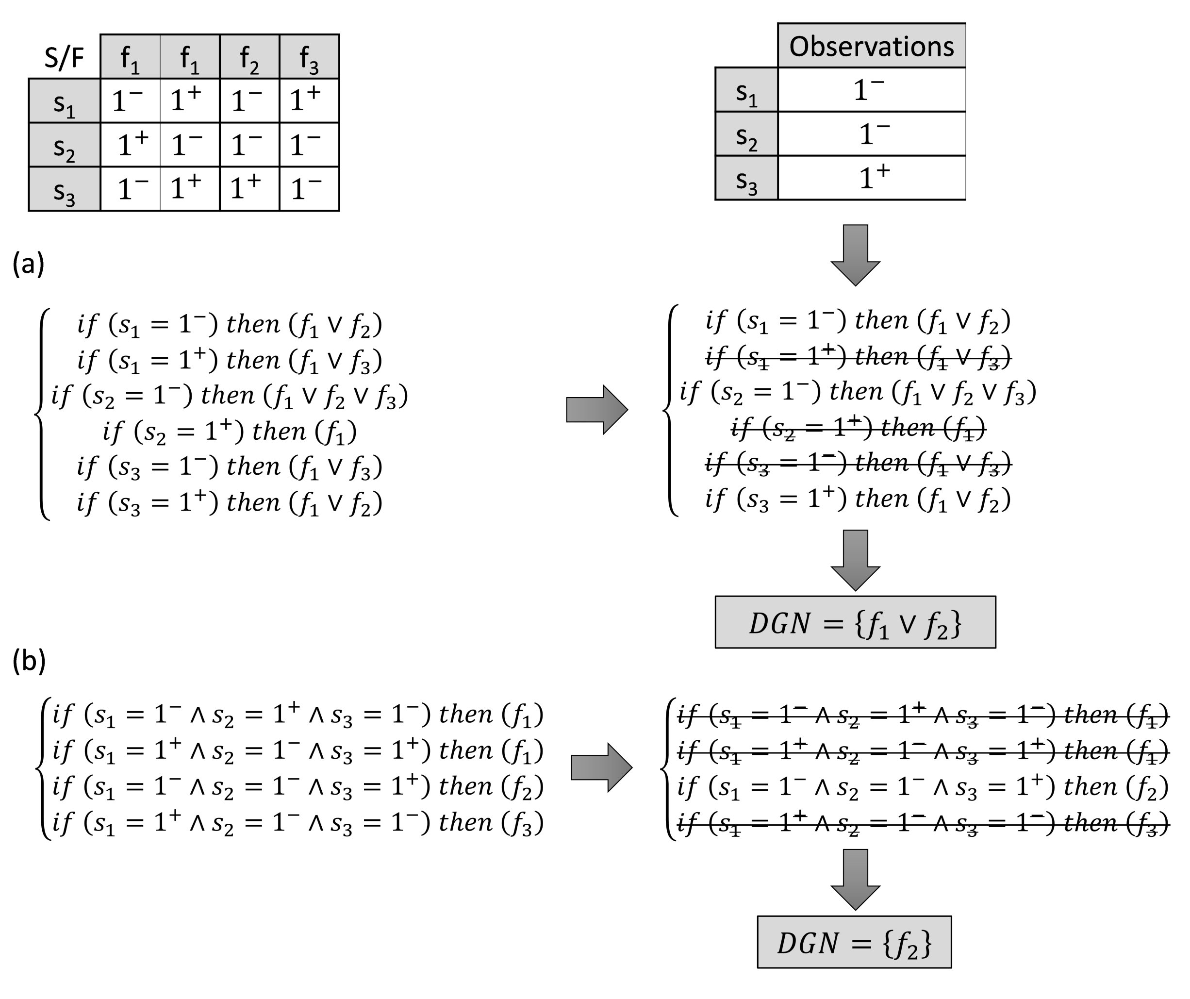
Signature-based reasoning provides higher fault distinguishability than row-based reasoning. The main reason for this is the use of the exoneration assumption, but not only that. It can be shown that even in the absence of zeros in the signatures, reasoning based on columns can provide higher distinguishability. This is illustrated by the example shown in Figure 1.
The reason for this is the use of additional information on the mutual relations of symptoms in simple signatures (Figure 1), which cannot be derived directly from the analysis of the rules corresponding to the FIS rows, as well as from columns in the form of complex signatures (13). Such a situation may occur only in the case of a multivalued residual assessment. When replacing a complex signature with simple signatures, it often turns out that some combinations of diagnostic signal values are physically impossible. The number of real simple signatures is smaller than the theoretical number of different combinations of diagnostic signal values. In theory, as shown in Section 5.2, eight simple signatures may appear for measurement faults f 8 , f 9 , f 10 , but only two are physically possible. The elimination of physically impossible combinations can lead to increased fault distinguishability.
The above statements regarding the distinguishability of faults are qualitative. There are a few examples of studies in which the impact of various elements of diagnostic reasoning algorithms on the indices of fault distinguishability were quantified. They are necessary for a more precise understanding of the impact of the methods of diagnosing and the properties of the diagnosed process on the indicators of distinguishing faults/states of the process;
2.
Resistance to symptom delays:
The problem of unequal delays of fault symptoms is well known and was analysed in [10,16,20,22,24,25,26,27]. Disregarding the dynamics of symptom formation may lead to the generation of temporary false diagnoses [10,22]. This applies to reasoning methods based on columns in which both symptoms and zero values of diagnostic signals are taken into account. The final diagnosis is made only in the steady state of all residuals. In transient states, the temporary values of diagnostic signals may indicate other faults/states of the process than the real one. This is how temporary false diagnoses arise.
All algorithms of reasoning based on rows, in which only fault symptoms are analysed, are resistant to symptom delays in the sense that they do not generate temporary false diagnoses;
3.
Resistance to structural changes (set of variables):
The method of reasoning also affects the resistance of the diagnostic system to structural changes of the diagnosed process, e.g., changes of the set of correctly functioning measurements. Measurement devices can be faulty or temporarily disconnected for calibration purposes, etc. The above changes result in the variability of the set of calculated residuals. In addition, each indication of an existing fault requires the introduction of automatic changes to the diagnostic system to ensure its proper functioning with a new process state. The set of active diagnostic signals should be reduced by those signals that are sensitive to the detected fault.
During the operation of the diagnostic system, the generated set of residuals changes. This leads to the necessity to change the fault signatures accordingly. Without such changes, column-based reasoning is not resistant to the structural changes of the diagnosed process. Moreover, in the case of large-scale systems, where the number of calculated residuals is very large, the signatures corresponding to the columns of the binary diagnostic matrix or information system are inconvenient, due to their large size.
A resistant method of notation of the diagnostic relationship in terms of possible changes in the structure of the object is the rules of the form of (14) and (15), in which particular symptoms are assigned to subsets of faults causing these symptoms. This relationship does not change. In the case of changes in the structure of the process or as a result of previous diagnoses, such a rule may be temporarily eliminated from the set of active rules, but its form remains unchanged. Moreover, such a rule has a compact form, also because the number of possible faults indicated in the conclusion is not large, in the case of using partial models;
4.
Resistance to compensation effect:
The compensation effect occurs in the case of multiple faults, when the influences of two or more faults compensate for each other and the residual value does not exceed the decision threshold. This phenomenon can occur only when the signs of the fault influence on the residual are opposite.
Reasoning based on columns with binary diagnostic signals is not immune to the compensation effect. The DX method assumes the possibility of compensation of the fault influence on the residual; however, the signs of fault interaction on the residuals are not taken into account. Therefore, the property of correct reasoning commonly attributed to this method in situations of fault compensation sometimes fails. Potentially incorrect diagnoses, inconsistent with the existing state, may be generated, which was demonstrated in [19]. It was shown that diagnosing on the basis of the three-value residual assessment was an effective method of eliminating reasoning errors caused by compensation effects. The rules for determining signatures for states with double faults are given;
5.
Possibility of making diagnoses inconsistent with the actual state:
The binary assessment of the residual values/conflicts in the FDI and DX approaches may be the cause of incorrect diagnoses, not necessarily related to the compensation effect [19]. Logically correct, but physically impossible diagnoses arise even in the absence of modelling errors, disturbances, and measurement noise. The reason for this is the loss of information about the residuum sign. The use of the three-value residual assessment and the principle of determining signatures for states with double faults given in the above work eliminate such diagnoses.

4. Column Reasoning Based on the Fault Isolation System and Elementary Symptoms’ Sequence: The New Method of Reasoning

4.1. Assumptions

  • The relationship between the faults and the diagnostic signals in the form of the FIS is known;
  • Complex signatures derived from the FIS are transformed into a set of simple, physically possible signatures;
  • Some relationships between symptom delays and elementary sequences e s j , p f k s j , s p > are known. A set of these sequences is not usually complete;
  • It is assumed that the diagnostic signal is sensitive or not sensitive to the given fault. This means that if the subset V j k contains 0, it is a single-element set (it does not contain any other diagnostic signal value that is a symptom of the fault);
  • It is assumed that if a symptom occurs, it does not disappear at the end of the reasoning process;
  • In the reasoning process, a state without faults and single-fault states are considered. In the case of multiple faults, the complication of the sequence of symptoms is so great that it cannot be determined by an expert. The lack of a solution in the class of single faults results in the necessity to conclude with an increasing number of faults, based solely on the values of the diagnostic signals. In this case, the HS tree algorithms [15] can be used;
  • In the nth step (moment) of reasoning, two diagnoses are made in parallel: a diagnosis D G N n based on all values of the diagnostic signals s j S and a diagnosis D G N O S n solely based on the symptoms;
  • The complex signature Q f k = [ V 1 k , , V j k , , V J k ] T is converted into a set of simple signatures:
    Q f k = { Q p ( f k ) } ,
    where only those simple signatures that can physically exist are taken into account:
    Q p ( f k ) = [ v 1 p k , , v j p k , , v J p k ] T .

4.2. Principles of Formulating the Diagnosis

Physically possible, simple signatures of faults Q p ( f k ) and known elementary sequences stored in the knowledge base are used to formulate the diagnosis in steps. Each newly detected symptom starts another step of reasoning. In a given nth step, three stages of reasoning can be distinguished:
  • Recording of the symptom w j n 0 and all current diagnostic signal values:
    W n = [ w 1 n , , w j n , , w J n ] T ;
  • Determination of a pair of instantaneous diagnoses D n and D O S n based on the current values of the diagnostic signals;
  • Reduction of the sets indicated in the diagnoses from Step 2 as a result of the analysis of elementary sequences containing the last observed symptom w j n . In this phase, the following diagnoses are generated: D G N n and D G N O S n . As an aid, the set of faults that are impossible due to the observed sequences F O S ¯ is determined.
The reasoning process is completed after all diagnostic signal values have been determined. The last temporary diagnosis is the final diagnosis.
The first ( n = 1 ) symptom w j 1 0 detected initialises a fault isolation algorithm, and each subsequent w g n 0 symptom begins a new reasoning step. This corresponds to Phase (1) of the reasoning procedure.
In Phase (2), the D n diagnosis is made based on a comparison of the current values of diagnostic signals W n with simple signatures of all faults Q p ( f k ) :
D n = { f k : Q p f k = W n } .
This diagnosis may be an empty set in cases where the current values of the diagnostic signals do not match any fault signature. Due to the symptom delays, it may also indicate a fault other than the existing one. The diagnosis D O S n indicates faults with signatures where all observed symptoms are present. Diagnostic signals with a value of zero are disregarded. In the first step, it has the form:
D O S 1 = f k : w j 1 = v j p k .
In the next steps, only the faults indicated in the previous step of this diagnosis are taken into account:
D O S n = { f k D O S n 1 : w g n = v g p k } .
In Phase (3), the possibility of reducing diagnoses based on elementary sequences is analysed. In this case, the following reasoning applies to the last detected symptom w g n 0 : if there is an elementary sequence e s g , a f l = < s g , s a > , this means that the fault f l activates the symptom s g = w g first and then the symptom s a . If the symptom s g did not occur, but the symptom s a was detected, then the fault f l should be eliminated from the set of faults indicated in the diagnosis. Therefore, the set of faults that are impossible, due to the observed sequences F ¯ O S n , has the following form:
F ¯ O S n = { f l D n : e s g , a f l = s g , s a } .
Diagnoses are determined by the following formulas:
D G N n = D n { f l D n : e s g , a f l = s g , s a } ,
D G N O S n = D O S n { f l D O S n : e s g , a f l = s g , s a .
In the above algorithm, when formulating diagnoses D G N n based on the columns, only simple signatures are taken into account, which are allowed due to physical constraints. This guarantees higher fault distinguishability in comparison to the algorithms presented in [13].

5. Example

5.1. Diagnosed Process

The comparison of the new method with other known methods is carried out on the example of diagnosing the process shown in Figure 2. It is a group of serially connected liquid buffer tanks. The same object was used in [5] to compare the methods of inference based on rows. This makes it possible to compare the diagnostic accuracy indicators for these two groups of algorithms.
The processes taking place in the system of serially connected tanks [29,33,34,35] are simple for analytical modelling and, moreover, relatively complicated due to the feedback in the diagnosed process itself. Therefore, simulators of this process are often used in the comparative research of diagnostic methods.
The flow between tanks is given by:
F i = α i S i 2 g ( L i L i + 1 )
where:
  • α i —flow coefficient;
  • S i —flow cross-section;
  • g—acceleration due to gravity.
F 1 is an input flow forced by the pump.
In the conducted experiments, the values of flows are expressed in L/min and levels in m.
The change in volume in the ith tank is expressed as:
A i d L i d t = F i F i + 1
where A i is the cross-sectional area of the tank.

5.2. Diagnostic System Components

A brief description of the components of the diagnostic system in relation to the work [5] are provided so that the operation of the proposed diagnostic algorithm can be analysed.
The process diagnostics was carried out on the basis of three available measurements: flow F 1 and levels L 1 and L 4 . The partial parametric models with the following structure were used for the residuals’ calculation: L 1 = q 1 ( F 1 ) , L 4 = q 2 ( F 1 ) , and L 4 = q 3 ( L 1 ) . It was assumed that fuzzy TSK models, based on experimental data, would be used. These models were identified and validated using several datasets divided into training, test, and validation data.
The corresponding residuals are:
r 1 = L 1 q 1 ( F 1 )
r 2 = L 4 q 2 ( F 1 )
r 3 = L 4 q 3 ( L 1 )
The set of faults (Table 4) includes leaks from tanks, clogging of channels connecting the tanks, and measurement devices’ faults.
The sensitivity of particular residuals to faults is described by the dependencies:
r 1 = r 1 ( f 1 , f 2 , f 3 , f 4 , f 5 , f 6 , f 7 , f 8 , f 9 )
r 2 = r 2 ( f 1 , f 2 , f 3 , f 4 , f 5 , f 6 , f 7 , f 8 , f 10 )
r 3 = r 3 ( f 2 , f 3 , f 4 , f 6 , f 7 , f 9 , f 10 )
The binary diagnostic matrix for a considered process is presented in Table 5.
It can be concluded that the faults f 9 and f 10 can be distinguished, on the basis of the analysis of binary signatures, while the faults in the following subsets: { f 1 , f 8 } , { f 2 , f 3 , f 4 , f 5 , f 6 , f 7 } are indistinguishable.
A Fault Isolation System (FIS), developed with the assumption of a three-value assessment of residuals, is shown in Table 6. The simple signatures of physically possible faults are listed in Table 7.
Based on the analysis of the signatures in the FIS, it can be seen that faults f 9 and f 10 are unconditionally distinguishable, the faults in the subsets { f 2 , f 3 , f 4 } , { f 5 , f 6 , f 7 } are unconditionally distinguishable, and the faults in the subset { f 1 , f 8 } are conditionally distinguishable.
As in the work [5], the elementary sequences were defined and listed in Table 8, based on the GP and assuming the same geometric parameters of the tanks and the pipelines connecting them. The effects of sensor faults on the residual values were immediate; therefore, the sequences for these faults are not defined.
Table 9 lists pairs of elementary sequences that distinguish faults.
It should be noted that elementary sequences ensure the distinguishability of the following fault pairs (among others): f 2 and f 3 , f 2 and f 4 , f 2 and f 7 , f 3 and f 5 , f 4 and f 5 , and f 5 and f 7 , which are not distinguishable on the basis of binary signatures, and pairs f 2 and f 3 , f 2 and f 4 , and f 5 and f 7 , which are indistinguishable on the basis of three-value signatures.

5.3. Examples of Reasoning Based on the Proposed Algorithm

Below are examples of the diagnostic reasoning according to the proposed algorithm. A simulator of the diagnosed object was used in the research.
Example 1.
Figure 3 shows the plots of residuals and diagnostic signals for the f 1 fault simulation. The following sequence of symptoms was recorded: s 1 , s 2 . The course of reasoning is given in Table 10.
Remark 1.
  • The following elementary sequences were used in Step 1c: e s 1 , 2 f 1 = s 1 , s 2 ,
    e s 1 , 2 f 3 = s 2 , s 1 . They eliminate the possibility of faults f 3 and f 4 , as the first symptom of these faults would be s 2 = 1 , not s 1 = 1 ;
  • Temporary diagnoses D O S 1 and D O S 2 contain existing faults and are therefore genuine;
  • Final diagnoses D G N 2 D G N O S 2 are not the same due to the nature of the signatures in the FIS and the lack of a sequence to distinguish between faults f 1 and f 2 .
Example 2.
Figure 4 shows the plots of residuals and diagnostic signals for the fault f 5 simulation. The following sequence of symptoms was recorded: s 1 , s 3 , s 2 . The course of reasoning is given in Table 11.
Remark 2.
  • In Steps 1c and 3c, for the elementary sequences e s 1 , 2 f 7 = s 2 , s 1 and e s 1 , 3 f 7 = s 3 , s 1 , the fault f 7 is eliminated from the diagnosis;
  • Temporary diagnosis D G N 2 = f 9 is false. Temporary diagnoses D O S 1 , D O S 2 , and D O S 3 contain existing faults and are therefore genuine;
  • Final diagnoses are equal and indicate indistinguishable faults f 5 and f 6 .
Example 3.
Figure 5 shows the plots of residuals and diagnostic signals for the fault f 7 simulation. The following sequence of symptoms was recorded: < s 2 , s 1 > and < s 3 , s 1 > . Symptoms s 2 and s 3 appear in a such a short delay from each other that it is impossible to determine their sequence. The course of reasoning is given in Table 12.
Remark 3.
  • In Step 1c for the elementary sequences: e s 1 , 2 f 2 = s 1 , s 2 , e s 1 , 2 f 5 = s 1 , s 2 , e s 1 , 3 f 2 = s 1 , s 3 and e s 1 , 3 f 5 = s 1 , s 3 , the faults f 2 and f 5 are eliminated from the diagnosis.
  • Temporary diagnosis D G N 1 = f 10 is false. Temporary diagnosis D O S 1 contains existing faults and is therefore genuine;
  • Final diagnoses are equal and indicate indistinguishable faults f 6 and f 7 .

6. Comparison of the Method with Others in Terms of the Obtained Fault Distinguishability

The following methods were taken into account for the comparison: CR-FSM, CR-FSM-ES, CR-FIS, and CR-FIS-ES. According to the authors’ knowledge, the CR-FSM-ES method has not been presented so far. Table 13 summarises the diagnoses obtained with the use of various methods of inference based on the columns.
On the basis of Table 13, the distinguishability of faults in the case of the considered object and the analysed diagnostic methods can be compared. The diagnostic accuracy index D [5], defined as the mean accuracy of diagnosis for all K faults, was used as a measure of distinguishability.
D = 1 K i = 1 K 1 d i
The accuracy of a single diagnosis is defined as the reciprocal of the number of faults d i indicated in the diagnosis. Thus, the accuracy of the isolation of the fault f i is the average value of the accuracy of diagnoses generated in the event of this fault.
Table 14 presents the calculated values of the diagnosis accuracy index D for the studied methods of inference based on Columns (CR) and compared them with the values of this indicator when making inference based on Rows (RR) determined in [5].
Table 14 shows an increase in the value of the diagnostic accuracy index when using the FIS instead of the FSM and the knowledge of elementary symptom sequences. The highest value of the diagnostic accuracy index D, which is a measure of fault distinguishability, was obtained for the newly proposed CR-FIS-ES method. The increment of the values in relation to the classical algorithm of inference, based on columns with the use of the FSM, was 0.275 (over 68%).
The aim of the article was also to compare the results obtained by inference methods based on columns and rows. The comparison was possible because the same diagnosed process and the same set of models for fault detection were used in the research. Table 14 shows that the methods of reasoning based on columns ensured a higher distinguishability of faults, compared to the methods of reasoning based on rows.
One of the disadvantages of reasoning based on signatures is false diagnoses generated in the transient states of diagnostic signals, before their final value is established. However, because of the second parallel reasoning process, the new method provides a diagnosis D G N O S n containing the existing fault. The presented fault isolation method allowed us to obtain the highest distinguishability of faults in the case of the analysed object among all the methods. This proves the effectiveness of the proposed algorithm.

7. Discussion and Conclusions

This paper presented a new method of diagnostic reasoning based on columns, in which three-value diagnostic signals and knowledge about the sequence of symptom formation for individual faults were used. The knowledge about sequences does not have to be complete. Only known elementary sequences were used.
The reasoning algorithm was implemented in a stepwise manner, after observing subsequent symptoms. At each reasoning step, two diagnoses were formulated in parallel: diagnosis D G N n based on all values of diagnostic signals s j S and diagnosis D G N O S n solely on the basis of symptoms. Temporary diagnoses D G N n may be false, but the final diagnosis made after all symptoms emerged is true. On the other hand, temporary diagnoses D G N n C O S always contain the existing fault.
The proposed method allows the increase of the obtained fault distinguishability, in relation to other known methods. The increase in distinguishability is greater the more complete is the knowledge of the elementary symptoms’ sequences.
High distinguishability of faults in the diagnostic reasoning is essential for the safety of the diagnosed process. Precise indications of faults in diagnoses allow taking effective actions to protect against the occurrence of dangerous failures.
The obtained results contribute to the increase of knowledge on the methods of increasing fault distinguishability in the diagnostics of dynamic systems. The proposed method can be easily applied in industry. It does not require models that take into account the impact of faults on the residuals. It uses knowledge and data that can be obtained relatively simply from specialists who understand the diagnosed process.
It is worth underlining that the proposed approach makes it possible to diagnose not only faults, but also cyber attacks aimed at falsifying measurement data. Assuming that the cyber attack will result in false measurement values in the automation system, the described method will generate information about the fault: there will be residuals deviating from the normal values, and related symptoms will appear. In the classic approach, the effect of such a cyber attack is indistinguishable from measuring device fault. However, taking into account the multivalued residuals’ assessment and the sequence of symptoms can lead to the possibility of distinguishing fault from cyber attack. This is a hypothesis that requires verification in the course of further research. The method, unlike others [36], does not require knowledge of the mathematical model of the process.
The direction of further work should focus on increasing the resistance of the method to the uncertainty of symptoms. The sources of these uncertainties are: variability of process model parameters, measurement disturbances and noise, and difficulties in determining threshold values. Further work is expected to introduce the fuzzy approach or to apply the Dempster–Shafer theory to address symptom uncertainty problems.

Author Contributions

Conceptualisation, methodology, and writing—original draft, J.M.K. and M.S.; formal analysis, J.M.K.; data curation and software, M.S.; validation and investigation, M.S., P.W. and M.S.; writing—review and editing, P.W., M.S. and J.M.K.; visualisation, M.S.; supervision, J.M.K. All authors have read and agreed to the published version of the manuscript.

Funding

The project was funded by the POB Research Centre for Artificial Intelligence and Robotics at the Warsaw University of Technology, within the Excellence Initiative Program-Research University (ID-UB).

Informed Consent Statement

Not applicable.

Data Availability Statement

Not applicable.

Conflicts of Interest

The authors declare no conflict of interest. The funders had no role in the design of the study; in the collection, analyses, or interpretation of the data; in the writing of the manuscript; nor in the decision to publish the results.

References

  1. Kościelny, J.M.; Bartyś, M.; Sztyber, A. Diagnosing with a hybrid fuzzy-bayesian inference approach. Eng. Appl. Artif. Intell. 2021, 104, 104345. [Google Scholar] [CrossRef]
  2. Buciakowski, M.; Witczak, M.; Mrugalski, M.; Theilliol, D. A quadratic boundedness approach to robust DC motor fault estimation. Control Eng. Pract. 2017, 66, 181–194. [Google Scholar] [CrossRef]
  3. Pulido, B.; Zamarreo, J.; Merino, A.; Bregon, A. State space neural networks and model-decomposition methods for fault diagnosis of complex industrial systems. Eng. Appl. Artif. Intell. 2019, 79, 67–86. [Google Scholar] [CrossRef]
  4. Talaat, M.; Gobran, M.; Wasfi, M. A hybrid model of an artificial neural network with thermodynamic model for system diagnosis of electrical power plant gas turbine. Eng. Appl. Artif. Intell. 2018, 68, 222–235. [Google Scholar] [CrossRef]
  5. Kościelny, J.M.; Syfert, M.; Wnuk, P. Diagnostic Row Reasoning Method Based on Multiple-Valued Evaluation of Residuals and Elementary Symptoms Sequence. Energies 2021, 14, 2476. [Google Scholar] [CrossRef]
  6. Pazera, M.; Witczak, M.; Kukurowski, N.; Buciakowski, M. Towards Simultaneous Actuator and Sensor Faults Estimation for a Class of Takagi-Sugeno Fuzzy Systems: A Twin-Rotor System Application. Sensors 2020, 20, 3486. [Google Scholar] [CrossRef]
  7. Łabęda-Grudziak, Z.M.; Lipiński, M. The identification method of the coal mill motor power model with the use of machine learning techniques. Bull. Ploish Acad. Sci. Tech. Sci. 2021, 69, e135842. [Google Scholar] [CrossRef]
  8. Cho, S.; Jiang, J. A fault detection and isolation technique using nonlinear support vectors dichotomizing multi-class parity space residuals. J. Process Control 2019, 82, 31–43. [Google Scholar] [CrossRef]
  9. Cordier, M.O.; Dague, P.; Lévy, F.; Montmain, J.; Staroswiecki, M.; Travé-Massuyès, L. Conflicts versus analytical redundancy relations: A comparative analysis of the model based diagnosis approach from the artificial intelligence and automatic control perspectives. IEEE Trans. Syst. Man Cybern. Part A Syst. Hum. 2004, 34, 2163–2177. [Google Scholar] [CrossRef]
  10. Puig, V.; Schmid, F.; Quevedo, J.; Pulido, B. A New Fault Diagnosis Algorithm that Improves the Integration of Fault Detection and Isolation. In Proceedings of the 44th IEEE Conference on Decision and Control, Seville, Spain, 15 December 2005; pp. 3809–3814. [Google Scholar] [CrossRef]
  11. Travé-Massuyès, L. Bridges between diagnosis theories from control and AI perspectives. In Intelligent Systems in Technical and Medical Diagnostics; Springer: Berlin/Heidelberg, Germany, 2014; Volume 230, pp. 3–28. [Google Scholar] [CrossRef]
  12. Blanke, M.; Kinnaert, M.; Lunze, J.; Staroswiecki, M. Diagnosis and Fault-Tolerant Control; Springer: New York, NY, USA, 2015. [Google Scholar]
  13. Korbicz, J.; Kościelny, J.M.; Kowalczuk, Z.; Cholewa, W. Fault Diagnosis: Models, Artificial Intelligence Methods, Applications; Springer: Berlin/Heidelberg, Germany, 2004. [Google Scholar]
  14. Kościelny, J.M.; Bartyś, M.; Rzepiejewski, P.; Sá da Costa, J. Actuator fault distinguishability study for the DAMADICS benchmark problem. Control Eng. Prac. 2006, 14, 645–652. [Google Scholar] [CrossRef]
  15. Reiter, R.A. Theory of Diagnosis from First Principles. Artif. Intell. 1987, 32, 57–95. [Google Scholar] [CrossRef]
  16. Syfert, M.; Kościelny, J.M. Diagnostic Reasoning Based on Symptom Forming Sequence. IFAC Proc. Vol. 2009, 42, 89–94. [Google Scholar] [CrossRef]
  17. Kościelny, J.M.; Syfert, M.; Rostek, K.; Sztyber, A. Fault isolability with different forms of the faults–symptoms relation. Int. J. Appl. Math. Comput. Sci. 2016, 26, 815–826. [Google Scholar] [CrossRef] [Green Version]
  18. Bregon, A.; Biswas, G.; Pulido, B.; Alonso-Gonzalez, C.; Khorasgani, H. A common framework for compilation techniques applied to diagnosis of linear dynamic systems. IEEE Trans. Syst. Man Cybern. Syst. 2014, 44, 863–876. [Google Scholar] [CrossRef]
  19. Kościelny, J.M.; Bartyś, M.; Łabęda-Grudziak, Z. Tri-valued Evaluation of Residuals as a Method of Addressing the Problem of Fault Compensation Effect. In Advances in Diagnostics of Processes and Systems, Proceedings of the 14th International Conference on Diagnostics of Processes and Systems (DPS), Zielona Góra, Poland, 21–23 September 2020; Korbicz, J., Patan, K., Luzar, M., Eds.; Studies in Systems, Decision and Control; Springer: Cham, Switzerland, 2021; Volume 313, pp. 31–44. ISBN 3030589633. [Google Scholar] [CrossRef]
  20. Kościelny, J.M.; Zakroczymski, K. Fault Isolation Algorithm that Takes Dynamics of Symptoms Appearances into Account. Bull. Pol. Acad. Sci. Tech. Sci. 2001, 49, 323–336. [Google Scholar] [CrossRef]
  21. Kościelny, J.M.; Bartyś, M.; Rostek, K. The comparison of fault distinguishability approaches—Case study. Bull. Pol. Acad. Sciences. Tech. Sci. 2019, 67, 1059–1068. [Google Scholar] [CrossRef]
  22. Kościelny, J.M. Fault Isolation in Industrial Processes by Dynamic Table of States Method. Automatica 1995, 31, 747–753. [Google Scholar] [CrossRef]
  23. De Kleer, J. Hitting set algorithms for model-based diagnosis. In Proceedings of the 22th International Workshop on Principles of Diagnosis (DX-11), Murnau, Germany, 4–7 October 2011. [Google Scholar]
  24. Kościelny, J.M.; Syfert, M. The issue of symptom based diagnostic reasoning. In Recent Advances in Mechatronics; Springer: Berlin/Heidelberg, Germany, 2007; pp. 167–171. [Google Scholar]
  25. Combastel, C.; Gentil, S.; Rognon, J.P. Toward a better integration of residual generation and diagnostic decision. IFAC Proc. Vol. 2003, 36, 69–74. [Google Scholar] [CrossRef]
  26. Daigle, M.; Koutsoukos, X.; Biswas, G. Relative Measurement Orderings in Diagnosis of Distributed Physical Systems. In Proceedings of the 43rd Annual Allerton Conference on Communication, Control, and Computing, Monticello, IL, USA, 28–30 September 2005; pp. 1707–1716. [Google Scholar]
  27. Meseguer, J.; Puig, V.; Escobet, T. Fault Diagnosis using a Timed Discrete Event Approach based on Observers. IFAC Proc. Vol. 2008, 41, 6914–6919. [Google Scholar] [CrossRef]
  28. Biswas, G.; Koutsoukos, X.; Pulido, B.; Bregon, A. Analytic redundancy, possible conflicts, and tcg-based fault signature diagnosis applied to nonlinear dynamic systems. IFAC Proc. Vol. 2009, 42, 1486–1491. [Google Scholar] [CrossRef] [Green Version]
  29. Bregon, A.; Biswas, G.; Pulido, B. A Decomposition Method for Nonlinear Parameter Estimation. IEEE Trans. Syst. Man Cybern. Part A Syst. Hum. 2012, 42, 751–763. [Google Scholar] [CrossRef]
  30. Sztyber, A.; Ostasz, A.; Kościelny, J.M. Graph of a Process-a new tool for finding model’s structures in model based diagnosis. IEEE Trans. Syst. Man Cybern. Syst. 2015, 45, 1004–1017. [Google Scholar] [CrossRef]
  31. Straka, O.; Punčochář, I. Decentralized and distributed active fault diagnosis: Multiple model estimation algorithms. Int. J. Appl. Math. Comput. Sci. 2020, 30, 239–249. [Google Scholar] [CrossRef]
  32. Xu, F.; Puig, V.; Ocampo-Martinez, C.; Olaru, S.; Niculescu, S.-I. Robust MPC for actuator-fault tolerance using set-based passive fault detection and active fault isolation. Int. J. Appl. Math. Comput. Sci. 2017, 27, 43–61. [Google Scholar] [CrossRef] [Green Version]
  33. Daigle, M.; Bregon, A.; Koutsoukos, X.; Biswas, G.; Pulido, B. A qualitative event-based approach to multiple fault diagnosis in continuous systems using structural model decomposition. Eng. Appl. Artif. Intell. 2016, 53, 190–206. [Google Scholar] [CrossRef]
  34. Bregon, A.; Alonso-González, C.J.; Pulido, B. Integration of simulation and state observers for online fault detection of nonlinear continuous systems. IEEE Trans. Syst. Man Cybern. Syst. 2014, 44, 1553–1568. [Google Scholar] [CrossRef]
  35. Khorasgani, H.; Biswas, G.; Jung, D. Structural Methodologies for Distributed Fault Detection and Isolation. Appl. Sci. 2019, 9, 1286. [Google Scholar] [CrossRef]
  36. Taheri, M.; Khorasani, K.; Shames, I.; Meskin, N. Cyber Attack and Machine Induced Fault Detection and Isolation Methodologies for Cyber-Physical Systems. Comput. Sci. Eng. 2020, 10. [Google Scholar] [CrossRef]
Figure 1. Reasoning based on rules corresponding to: (a) rows or (b) columns (fault signatures) of the F I S .
Energies 15 02614 g001
Figure 2. Diagnosed process—a set of serially-connected liquid buffer tanks. Physical variables available for measurement are placed in the black boxes.
Energies 15 02614 g002
Figure 3. Examples of diagnosing the case of the f 1 fault: (a) residual values and (b) diagnostic signal values (three-value signal 1 , 0 , 1 scaled to an s j number).
Energies 15 02614 g003
Figure 4. Examples of diagnosing in the case of the f 5 fault: (a) residual values and (b) diagnostic signal values (three-value signal 1 , 0 , 1 scaled to an s j number).
Energies 15 02614 g004
Figure 5. Examples of diagnosing in the case of the f 7 fault: (a) residual values and (b) diagnostic signal values (three-value signal 1 , 0 , 1 scaled to an s j number).
Energies 15 02614 g005
Table 1. Example of the FSM.
S/F f 1 f 2 f 3 f 4
s 1 1 11
s 2 11
s 3 1 1
Table 2. Example FIS.
S/F f 1 f 2 f 3 f 4 V j
s 1 1011{0,1}
s 2 0=1−1, +1−1{0, +1, −1}
s 3 1, 2210{0, 1, 2}
Table 3. Replacement of a complex signature by a set of simple signatures.
S f k f k
s 1 1, 21212
s 2 00000
s 3 −1, +1−1−1+1+1
Table 4. A set of faults.
Fault SymbolDescription
f 1 leak from Tank 1
f 2 leak from Tank 2
f 3 leak from Tank 3
f 4 leak from Tank 4
f 5 clogging in the flow channel between Tanks 1 and 2
f 6 clogging in the flow channel between Tanks 2 and 3
f 7 clogging in the flow channel between Tanks 3 and 4
f 8 measurement F 1 fault
f 9 measurement L 1 fault
f 10 measurement L 4 fault
Table 5. Binary diagnostic matrix.
f 1 f 2 f 3 f 4 f 5 f 6 f 7 f 8 f 9 f 10
s 1 111111111
s 2 11111111 1
s 3 111111 11
Table 6. Fault Isolation System (FIS).
f 1 f 2 f 3 f 4 f 5 f 6 f 7 f 8 f 9 f 10
s 1 −1−1−1−1+1+1+1−1,+1−1,+1
s 2 −1−1−1−1−1−1−1−1,+1 −1,+1
s 3 −1−1−1−1−1−1 −1,+1−1,+1
Table 7. Physically possible three-value fault signatures.
f 1 f 2 f 3 f 4 f 5 f 6 f 7 f 8 f 9 f 10
+++
s 1 −1−1−1−1+1+1+1+1−1−1+1
s 2 −1−1−1−1−1−1−1+1−1 −1+1
s 3 −1−1−1−1−1−1 +1−1−1+1
Table 8. Elementary sequences for an object.
Fault SymbolDescription
f k Elementary Sequences
f 1 e s 1 , 2 f 1 = s 1 , s 2 ,
f 2 e s 1 , 2 f 2 = s 1 , s 2 , e s 1 , 3 f 2 = s 1 , s 3 ,
f 3 e s 1 , 2 f 3 = s 2 , s 1 , e s 1 , 3 f 3 = s 3 , s 1 ,
f 4 e s 1 , 2 f 4 = s 2 , s 1 , e s 1 , 3 f 4 = s 3 , s 1
f 5 e s 1 , 2 f 5 = s 1 , s 2 , e s 1 , 2 f 5 = s 1 , s 3 ,
f 6 none
f 7 e s 1 , 2 f 7 = s 2 , s 1 , e s 1 , 3 f 7 = s 3 , s 1 ,
Table 9. Pairs of elementary sequences that distinguish faults.
e s 1 , 2 f 1 = s 1 , s 2 , e s 1 , 2 f 3 = s 2 , s 1 e s 1 , 2 f 1 = s 1 , s 2 e s 1 , 2 f 4 = s 2 , s 1
e s 1 , 2 f 1 = s 1 , s 2 , e s 1 , 2 f 7 = s 2 , s 1
e s 1 , 2 f 2 = s 1 , s 2 , e s 1 , 2 f 3 = s 2 , s 1 e s 1 , 3 f 2 = s 1 , s 3 , e s 1 , 3 f 3 = s 3 , s 1
e s 1 , 2 f 2 = s 1 , s 2 , e s 1 , 2 f 4 = s 2 , s 1 e s 1 , 3 f 2 = s 1 , s 3 , e s 1 , 3 f 4 = s 3 , s 1
e s 1 , 2 f 2 = s 1 , s 2 , e s 1 , 2 f 7 = s 2 , s 1 e s 1 , 3 f 2 = s 1 , s 3 , e s 1 , 3 f 7 = s 3 , s 1
e s 1 , 2 f 3 = s 2 , s 1 , e s 1 , 2 f 5 = s 1 , s 2 e s 1 , 3 f 3 = s 3 , s 1 , e s 1 , 3 f 5 = s 1 , s 3
e s 1 , 2 f 4 = s 2 , s 1 , e s 1 , 2 f 5 = s 1 , s 2 e s 1 , 3 f 4 = s 3 , s 1 , e s 1 , 2 f 5 = s 1 , s 3
e s 1 , 2 f 5 = s 1 , s 2 , e s 1 , 2 f 7 = s 2 , s 1 e s 1 , 3 f 5 = s 1 , s 3 , e s 1 , 3 f 7 = s 3 , s 1
Table 10. The results of the algorithm for the input signals from Figure 3.
StepAlgorithm Results
1a s 1 = 1 ; W 1 = [ 1 , 0 , 0 ] T
b D 1 = ; D O S 1 = f 1 , f 2 , f 3 , f 4 , f 8 , f 9
c F ¯ O S 1 = f 3 , f 4 , f 7 D G N 1 = , D G N O S 1 = f 1 , f 2 , f 8 , f 9
2a s 2 = 1 ; W 2 = [ 1 , 1 , 0 ] T
b D 2 = f 1 , f 8 , D O S 2 = f 1 , f 2 , f 8
c F ¯ O S 2 = f 3 , f 4 , f 7 D G N 2 = f 1 , f 8 , D G N O S 2 = f 1 , f 2 , f 8
Table 11. The results of the algorithm for the input signals from Figure 4.
StepAlgorithm Results
1a s 1 = + 1 ; W 1 = [ + 1 , 0 , 0 ] T
b D 1 = ; D O S 1 = f 5 , f 6 , f 7 , f 8 , f 9
c F ¯ O S 1 = f 3 , f 4 , f 7 , D G N 1 = ; D G N O S 1 = f 5 , f 6 , f 8 , f 9
2a s 3 = 1 ; W 2 = [ + 1 , 0 , 1 ] T
b D 2 = f 9 ; D O S 2 = f 5 , f 6 , f 9
c F ¯ O S 2 = f 3 , f 4 , f 7 , D G N 2 = f 9 ; D G N O S 2 = f 5 , f 6 , f 9
3a s 2 = 1 ; W 3 = [ + 1 , 1 , 1 ] T
b D 3 = f 5 , f 6 , f 7 ; D O S 3 = f 5 , f 6
c F ¯ O S 2 = f 3 , f 4 , f 7 , D G N 3 = f 5 , f 6 ; D O S 3 = f 5 , f 6
Table 12. The results of the algorithm for the input signals from Figure 5.
StepAlgorithm Results
1a s 2 = 1 ; s 3 = 1 ; W 1 = [ 0 , 1 , 1 ] T
b D 2 = f 10 ; D O S 1 = f 2 , f 3 , f 4 , f 5 , f 6 , f 7 , f 10
c F ¯ O S 1 = f 1 , f 2 , f 5 ; D G N 1 = f 10 ; D G N O S 1 = f 3 , f 4 , f 6 , f 7 , f 10
2a s 1 = + 1 ; W 2 = [ + 1 , 1 , 1 ] T
b D 2 = f 5 , f 6 , f 7 ; D O S 2 = f 6 , f 7
c F ¯ O S 2 = f 1 , f 2 , f 5 ; D G N 2 = f 6 , f 7 ; D G N O S 2 = f 6 , f 7
Table 13. List of diagnoses obtained by reasoning methods based on columns.
f k Diagn. SignalsCR-FSMCR-FSM-ESCR-FISCR-FIS-ESDiagn. Signals
f 1 1 , 1 , 0 { f 1 , f 8 } { f 1 , f 8 } { f 1 , f 8 } { f 1 , f 8 } −1,−1, 0
f 2 1 , 1 , 1 { f 2 , f 3 , f 4 , f 5 , f 6 , f 7 } { f 2 , f 5 , f 6 } { f 2 , f 3 , f 4 } { f 2 } −1,−1,−1
f 3 1 , 1 , 1 { f 2 , f 3 , f 4 , f 5 , f 6 , f 7 } { f 3 , f 4 , f 6 , f 7 } { f 2 , f 3 , f 4 } { f 3 , f 4 } −1,−1,−1
f 4 1 , 1 , 1 { f 2 , f 3 , f 4 , f 5 , f 6 , f 7 } { f 3 , f 4 , f 6 , f 7 } { f 2 , f 3 , f 4 } { f 3 , f 4 } −1,−1,−1
f 5 1 , 1 , 1 { f 2 , f 3 , f 4 , f 5 , f 6 , f 7 } { f 2 , f 5 , f 6 } { f 5 , f 6 , f 7 } { f 5 , f 6 } +1,−1,−1
f 6 1 , 1 , 1 { f 2 , f 3 , f 4 , f 5 , f 6 , f 7 } { f 2 , f 5 , f 6 } or { f 3 , f 4 , f 6 , f 7 } * { f 5 , f 6 , f 7 } { f 5 , f 6 } or { f 6 , f 7 } *+1,−1,−1
f 7 1 , 1 , 1 { f 2 , f 3 , f 4 , f 5 , f 6 , f 7 } { f 3 , f 4 , f 6 , f 7 } { f 5 , f 6 , f 7 } { f 6 , f 7 } +1,−1,−1
f 8 1 , 1 , 0 { f 1 , f 8 } { f 1 , f 8 } { f 1 , f 8 } { f 1 , f 8 } −1, −1, 0
{ f 8 } { f 8 } +1, +1, 0
f 9 1 , 0 , 1 { f 9 } { f 9 } { f 9 } { f 9 } −1, 0, +1
{ f 9 } { f 9 } +1, 0, −1
f 10 0 , 1 , 1 { f 10 } { f 10 } { f 10 } { f 10 } 0,−1,−1
f 10 f 10 0, +1, +1
* Diagnosis depends on the observed sequence of symptoms.
Table 14. Summary of diagnostic accuracy indicators for the tested methods
Reasoning MethodFSMFSM-ESFISFIS-ES
CR0.4000.4700.5250.675
RR0.1540.2470.4000.538
Publisher’s Note: MDPI stays neutral with regard to jurisdictional claims in published maps and institutional affiliations.

