Water, Energy and Food Algorithm with Optimal Allocation and Sizing of Renewable Distributed Generation for Power Loss Minimization in Distribution Systems (WEF)

Abstract

Distributed generation (DG) plays a vital role in electrical power networks. However, power loss reduction, voltage profile improvement, friendly environment, and reliability are all benefits of DG units. In this research work, a worthwhile methodology is recommended for optimal allocation of traditional (gas turbine) and renewable energy sources that are based on distributed generators which include solar and wind in the distribution system. The major objective of the research paper is the minimization of real, reactive power losses and emissions produced during the application of these conventional sources. Originally, the best locations to place this DG are identified using the concept of water, energy, and food algorithm (WEFA). The number and sizes of these renewable energy sources selected (wind and solar) are determined by applying the concepts of the Dragonfly Algorithm. The Weibull and beta distribution functions are modeled to extract the exact position to fix our DGs to minimize losses within the distribution network. To assess the performance of WEF five different cases scenario considered are DG capacity, Location of Bus, voltage profile, maximum power loss as well as utilization rate. The proposed WEF Algorithm is tested on the IEEE standard 33-bus system. The simulated results were compared with others found in literature and found to be better in terms of power loss reductions.

1. Introduction

Distributed Generation has demonstrated an expanding measure of development in Power Distribution Network all over the world. This is because of the advancement in the usage of renewable energy resources and improvement in co-generation. This development has made DG more popular [1,2]. Distributed Generations are small-scale power generation sources that are connected directly to the Distribution Network (DN) and close to the consumer load being served [3]. Hence, the size of the DN can be increased by integrating renewable-based technology. For instance, biomass generations and solar photovoltaic cell’s needs [3,4], to provide dependable and cost-effective services directly to customers while ensuring power reduction losses, greenhouse gas emission, flexible voltage regulations, power quality, peak load shaving, and reliability enhancements [5].

However, bad allocations decrease the overall performance of the distribution system [6]. Thus, it gained attention especially on developing methodologies for power losses minimization. For details, see [7,8,9,10,11,12].

Additionally, various algorithms have been developed to handle the issues related to DG in DN. For instance, Particle swarm optimization [13,14,15], Artificial bee colony [16], Hybrid particle swarm optimization [17], Harmony Search Algorithm [18], Dynamic programming [19], Simulated Annealing [20], Mixed linear integer programming [21], Improved Analytical [22] and Analytical [9] are used to solve DG allocation issues for minimizing power losses. An analytical method based on the determination of power loss and minimization of real power losses allocation of both single and multiple DG in primary DN were presented in [9,22]. However, this method does not provide actual computational time.

Harmony search optimization algorithm was proposed to optimally locate and size the DG in radial DN to minimize the total power losses [23]. Simulated Annealing was used in [20], while optimal sizing and locating a DG in large-scale DN to minimize power loss sensitivity and optimal sitting is achieved by a low sensitivity factor (LSF) [24]. Hence, a comparison between loss sensitivity, index vector, and voltage sensitivity index was done to optimal locate and size the DG in DN.

However, the author only considers the case of the unity power factor without considering the optimal power factor. A particle swarm optimization was presented for both a single and multi-objective approach to determine a real position to place multiple DG in a DN to maximize power loss [25]. Nevertheless, if a careful selection is made on the placement of the DG, it will become a real optimum solution. Thus, a simple search algorithm proposed in [26], to investigate the possibility of connecting wind turbines in a radial distribution system, with technical objectives of boosting the stability of the system.

Subsequently, the Algorithm requires large computational time to obtain results and is only suitable for single-objective optimization problems. Ref. [19], proposes dynamic programming to find optimum DG location in the distribution system and to minimize total power loss and boost the reliability of the system for maximum profit. The clonal selection Algorithm was applied in [27], to determine optimal DG’s size and location in radial distribution system with the technical objective for maximization of energy savings.

Additionally in [28], optimization was proposed to address the issue of optimal sizing and sitting the DG in DN for voltage improvement, power losses, and Total harmonic distortions (THD). Ref. [29], proposed an artificial bee colony to provide a solution to output DG power and location to multiple DG sources. The Big Bang crunch optimization algorithm was adopted in [30], to find the optimal location and size of the DG to minimize power loss in a balanced and unbalanced distribution network system.

While distribution planning was adopted by [31], using a backtracking search algorithm to produce an optimum solution for DG installations to boost voltage profile and reduce power loss in the radial system. Hence, in this paper, a new Algorithm based on water, energy, and food was proposed and adopted from [32], to determine optimum size and placement of multiple DG’s and to minimize power losses that arise in placement of our DG’s in a non-optimal position in the distribution network.

Furthermore, a methodology was proposed for optimal multiple DG placement of Gas turbines (conventional) and renewable-based DGs such as (wind and solar) placement in DN operating at 0.8 power factor which is sufficient in reducing power losses and improvement of voltage profile within the specified constraints. The major objectives are to minimize total power loss and emissions produced by this conventional system. The modeling of this renewable energy system was carried out based on Weibull and beta distribution probability to determine to extract the power loss. In this research work, the best location for the placement of sources was determined using the Water, energy, and food algorithm adopted by [32].

2. Basic Water, Energy, and Food (WEF) Optimization Algorithm Review

2.1. Water, Energy, and Food (WEF)

The concept of the WEF algorithm was proposed by [33], it’s a mathematical model developed to handle issues related to open-but-restricted-environment (OBR-E), which helps in achieving a sustainable environment. It’s a strong model for predicting the state of an element combined at any time. In [34], the authors proposed water, energy, and food Algorithm to achieve a sustainable environment. In 2005, J. Diamond surmises that it is essential for human beings to think about how to solve a complicated problem within the environment using (WEF) [35]. Mohammad Al-Saidi and Nadir Ahmad affirm that this problem of achieving a sustainable environment includes water-energy-food linkage [36]. Hence, we tend to apply this concept to achieve a greater sustainable distributed energy system.

2.2. Dragonfly Algorithm (DFA)

In 2015 [37], Seyedali Mirjalii proposed a dragonfly algorithm. This algorithm was developed to monitor both the static and dynamic behavior of dragonflies. The search for foods marks the path of utilization and informs and guides others. These creatures find the optimal position and perform the task efficiently within their domain.

The static swarm creates a particular group and flies back over a small area and hunt for flying prey, while the dynamic swarm creates a massive number of dragonflies, which makes the swarm migrate in one positive over long distances.

These two phases can be mathematically expressed as follows:

$$let Ki be the search process of drangonflies during the search to avoid collision$$

• $K_i=-{{\displaystyle \sum }}_{j=1}^{N}X-X_j$
  X denotes the current position of the dragonflies,
  While $X_j$ is the jth neighboring individuals.
  N is the number of neighboring individuals
• The alignment fitness is computed as follows:
  Considering the movement velocity as Vi, in the matching process as searching is taking place.

  $$Vi=\frac{{\displaystyle {\sum }_{j=1}^N{X}_j-X}}{N}$$

  (1)
  Jth is the velocity of neighboring.
• The cohesion is computed to attract the swarm towards the middle point of the grouping swarm.

  $$Ci=\frac{{\displaystyle {\sum }_{j=1}^{N}Xj-X}}{N}$$

  (2)
  X is the current position of individual
  N is the number of Neighborhood
  $X_j$ Denotes the position at neighboring individual
• The food attraction $(f^{\ast })$ by the swarm is mathematically computed to, attract the swarm.

  $$f^{\ast }=X^{+}-X$$

  (3)
  X is the current position of the individual
  $X^{+}$ The position of the food attraction source
• During Food attraction, the enemy is always present and must put into consideration

  $$E^{\ast }=X^{-}+X$$

  (4)
  $X^{-}$ is the enemy position, while $X$ in the initial position.

Lastly, the behavior of dragonflies during the searching period is modeled by the five governing equations given above in Equations (39) and (43). However in the process of searching the position and movements of these flies are amended by using a two-step vector.

$$\Delta X_{t+1}=(kKi+vVi+cCi+f{f}^{\ast }+e{E}^{\ast })+w\Delta Xt$$

(5)

After calculating the step vector in Equation (6), the position of the vector can be updated below.

$$X_{t+1}=X_t+\Delta X_{t+1}$$

(6)

where t, Ki, Vi, Ci, fi, and Ei are the initial iteration, alignment, cohesion, food attraction, and enemy and distraction towards enemy outwards of ith individuals. Additionally, (k, v, c, f, and e) are the weighting factors for the different parameters. To assure the guarantee of convergence of the dragonflies during optimization, there is always a change in their adaptive weights. Equation (7) can be updated to obtain the position of the dragonflies as given below.

$$X_{t+1}=X_t+0.01\times \frac{r1\times \sigma }{{\left(r_2\right)}^{1/\beta }}\times X_t$$

(7)

$$\sigma =\left(\frac{\Gamma \left(1+\beta \right)}{\frac{(1+\beta )}{2}}\right)\times {\left(\frac{\sin \frac{\beta \pi }{2}}{\beta \times 2\times \frac{\beta -1}{2}}\right)}^{\frac{1}{\beta }}$$

(8)

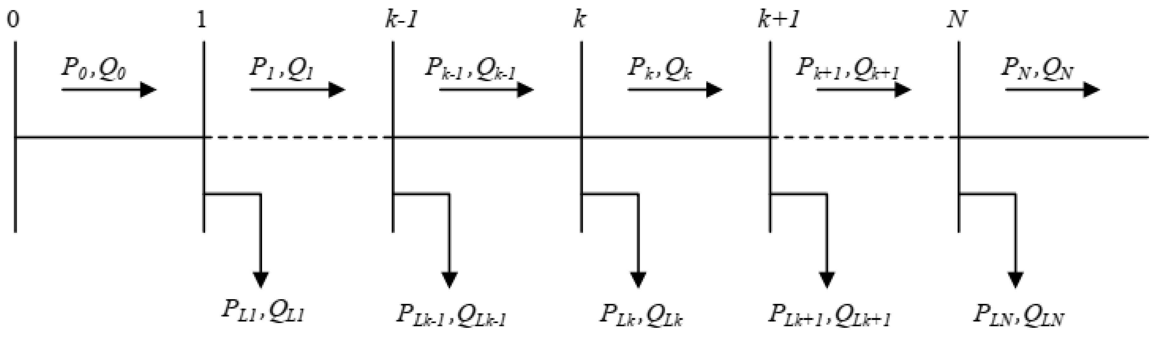
2.3. Active Power Loss Minimization

Electrical power energy is generated from a long-distance far away from the consumer side and is transported through the transmission line to many distribution circuits systems that the electrical utility operates on. Generally, the distribution network system will take power and sent it to the consumer of the load to serve their demands. However not all the power will be delivered 100 percent efficiently due to losses that occur at the distribution network line. The power loss in the distribution network system is dependent on the precise location and size of the Renewable DG system. The real power here is obtained and defined by [14].

$$E_{4}PLoss={\displaystyle {\sum }_j^{bn}{(Ij)}^2}Rj$$

(9)

where Ij and Rj are the current magnitude and resistance corresponding to the Jth branch, bn is the number of branches.

It is observed from Equation (10), that the total power loss will be affected when the line current changes. However, minimizing the total real power loss can be achieved by optimal placement and sizing. The renewable-based DG in the distribution system is defined by the Equation (11) below.

$$F_{Total}=\frac{P_{T}Loss+\mu }{MV{A}_{base}}$$

(10)

To normalize the total power loss MVA_base and µ are introduced which take a value between (0, 1) which is stated earlier.

$$PLDi\%(j)=\frac{PL(j)-PL\max }{PL(j)-PL\min }\times 100$$

(11)

where PLDi (j), PLmax and PLmin are the power loss index at bus j, power loss rejects at bus j, maximum power loss rejects and minimum power reject. The power loss index in Equation (12) is most likely to identify our DGs placement.

2.4. Constraints

The constraints imposed here is to solve the problems associated with optimal placement and sizing the DG in the distribution system. The bus cumulative magnitude voltage deviation (CVD) must be kept at a normalized value within specified limits at each particular bus as defined below.

$$\mathrm{CVD}=\left\{{\displaystyle {\sum }_{j=1}^{NDG’S}(1-vi)}\right., \mathrm{if} 0.95 \le vi\le 1.05\left.\right\}$$

(12)

The minimum of (0.95 pu) and maximum of (1.05 pu) voltage magnitude of each bus should be within the given limits.

$$\begin{gathered} V_{\min }\le V\le V_{(\max )} \\ \left|I_{K,K+1}\right|\ge I_{K,K+1(\max )} \end{gathered}$$

(13)

Equation (14) defines current limits carrying the line section between the buses of K and K + 1.

The current limits of the branches should be noted that they are not explicit and are defined by the IEEE bus.

Power flow constraints satisfaction

A simple radial feeder configuration is represented by the single line diagram in Figure 1. Power flow is computed with the aid of the following set of equations taking from [38].

$$P_{K+1}=P_K-P_{LK+1}-R_{K,K+1}\times \frac{P{K}^2+Q{K}^2}{\left|VK\right|\times \left|VK\right|}$$

(14)

$$Q_{K+1}=Q_K-Q_{LK+1}-Q_{LK+1}-X_{LK+1}{,}_L\times \frac{P^2{}_K+Q^2{}_K}{{\left|V_K\right|}^2}$$

(15)

$${\left|V_{K+1}\right|}^2={\left|V_k\right|}^2-2\times [R_{K,K+1}\times P_K+X_{K,K+1}\times Q]+⌊R_{{K,K+1}^2}+X_{K,K+1}⌋$$

(16)

$$P_{Load}+P_{Loss}=P_{subreal}+{\displaystyle {\sum }_{RDG=1}^{j}PRDG}$$

(17)

$$Q_{Load}+Q_{Loss}=Q_{Subreal}+{\displaystyle {\sum }_{RDG=1}^{j}QRDG}$$

(18)

DG perforation limit

$$PRDG\le PDemand$$

where $P_K$ the real power and $Q_K$ is the reactive power flowing through the bus K $P_{LK+1}$ is the real power demand, while $Q_{LK+1}$ is the reactive demand load at the peculiar bus called K + 1. Reactance and resistance of the line are $\left[R_{{K,K+1}^2},+,X_{K,K+1}\right]$ and. $\left|V_K\right|$, Is the magnitude of the voltage at the K bus. However, Equations (18) and (19) provide line losses connecting the bus Q.

The above constraints must always satisfy in the distribution network system, otherwise rejected.

2.5. Overall System Efficiency

To calculate the total efficiency η_System of the proposed system RDG in this work, we apply the concept of efficiency model in [38]. We let η_{j,j = 1,2,……n} denotes the component efficiencies for a given system with j components. Then the overall system energy efficiency η_System is given by

$${\eta }_{\mathit{\text{System}}}={\displaystyle \prod {\eta }_{j-k}}$$

(19)

3. Distributed Energy Resources Modelling (DER)

For the planning of various kinds of Renewable energy sources (RES), three (3) different optimization formulations have been adopted. The objectives used in this optimization technique are considered as maximization of energy utilization of Gas turbine, photo-voltaic system (PV) and wind turbine generation. The formulation is based on water, energy and food techniques adopted by having eight possible points to position our DGs within a given distribution network system.

3.1. Problem Formulation for Proposed Algorithm

The proposed Algorithm here, tells how the energy is utilized or under-utilized in a distribution network. The Algorithm predicts the state of an object relative to its usage at any given number of elements within the network system. However, this model is deployed to address global problems related to allocating multiple DGs in a given network system. This model has eight (8) possible coordinates to fix an object in a given network system, thereby minimizing energy loss.

The WEF model design for the allocation of the hybrid Renewable energy-based DG has some unique properties if fixed within the distribution network nodes.

• It has an infinite number of solutions and this has made it simple to fix our DG in many points within the Distribution system.
• A probabilistic solution generates several solutions for the whole WEF Renewable hybrid DG, thereby providing an optimal solution to minimize energy loss.

Here we assumed a state of three elements (water, energy, and food) that are interdependent on one another. However, these three states will form a natural communication Markov as proposed in [33]. The following notations are adopted:

• β: Denotes the constant values of the energy in wind
• γ: Denotes the constant values of solar energy
• α: Denotes the fuel cell energy constants
• ρ: Probabilitymeasuresontheenergyspaceforthe3DG^’ s such that Ei(:)i = 0,1
• μ: rate at which an element is used in the Distribution system
• L: The state of wind energy DG in a Distribution System
• i: The state of solar energy DG in a Distribution network system
• j: The state of fuel energy DG in a Distribution network system.

P 0, 0, 0: probability measure allocation of the DGs is maximum utilized in the distribution network.

P 1, 0, 0: probability measure that wind energy is maximum utilized, solar and gas turbines are minima utilized.

P 0, 1, 0: probability measure that solar is maximum utilized, while wind and gas turbines are minima utilized.

P 0, 0, 1: probability measure that gas turbine is maximum utilized, while solar and wind energy is minimum utilized.

P 1, 1, 0: probability measure that both solar and wind energy are maximum utilized, while gas turbine is minimum utilized.

P 0, 1, 1: probability measure that wind and gas turbines are maximum utilized, while solar energy is under-utilized.

P 0, 0, 1: probability measure that gas turbine is maximum utilized, while solar and wind energy is under-utilized.

P 1, 1, 1: probability measure that the 3 DGs is maximum utilized

In general

$$Ei=hc\sum Pi$$

(20)

E-Energy at [P 0, 0, 0], [P 1, 0, 0], [P 0, 1, 0], [P 1, 1, 0], [P 1, 0, 1], [P 0, 1, 1], [P 0, 0, 1], [P 1, 1, 1].

Emax is the monoticity, for the Emax to hold Ei > Ej.

3.2. Objective Functions Formulations

Case A: Minimization of wind energy

$$E(w)=E0,1,0(w)+E0,1,1(w)+E1,1,0(w)+E1,1,1(w)$$

(21)

Case B: Minimization of the solar PV system

$$E2(s)=E1,0,0(s)+E1,1,0(s)+E1,0,1(s)+E1,1,1(s)$$

(22)

Case C: Minimization of Gas Turbine energy system

$$E3=E0,0,1(f)+E0,1,1(f)+E1,0,1(f)+E1,1,1(f)$$

(23)

3.3. Wind Speed Modeling and Power Output

The real output power of the wind DG based is always immensely influenced by wind speed. Therefore, before the placement of these energy sources in the distribution system the uncertainty related to the speed of the energy is modeled. The wind power function is taken from [40].

$$P_{Wind}=0.5\rho ACpNgNb$$

Here Cp = Coefficient of performance

g = generator efficiency

Nb = gear box efficiency

ρ = density

A = Area

Let P be a probability of measure on the energy space for the wind DG, such that

$$\left\{Ei\left(:\right) :i=0,1\right\}$$

$$P\left(E1\left(w\right)\right.)=probability \mathrm{that} \mathrm{wind} \mathrm{DG} \mathrm{energy} \mathrm{is} \mathrm{at} \mathrm{maximum}$$

Application of the model, by [33], for a DG to attained maximum it must certify the Lagrangian function.

By Hamilton’s variation principle on Equation (22), the probability of the total energy is given by the Lagrangian function along the extreme path (maximum or minimum) compared to the nearby variation.

$${\displaystyle {\int }_0^{1}0.5\delta ANg\rho \partial \rho }$$

(24)

We assume $CP\to \rho$

$${{\displaystyle \int }}_0^{\infty }A Ng Nb f\left(\rho \right)\partial \rho =P\left(E0,1,0\right)+P\left(E0,1,1\right)+P\left(E,1,1,0\right)+P\left(E1,1,1\right)\left(4\right)$$

(25)

We assume

$$\beta =0.5\delta ANgNb$$

where $F\left(\rho \right) \mathrm{is} \mathrm{the} \mathrm{Langranrian} \mathrm{function}$

$$(\rho ,w)=\beta {\displaystyle \underset{0}{\overset{\infty }{\int }}f(\rho )\partial \rho =\frac{\pi \rho }{{(1+\rho )}^3(1+\pi +{\pi }^2)}}+\frac{\pi \rho (\pi +1)}{{(1+\rho )}^3(1+\pi +{\pi }^2)}+\frac{\rho (\pi +1)}{{(1+\rho )}^3(1+\pi +{\pi }^2)}+\frac{{\rho }^3}{(1+{\rho }^3)}$$

(26)

Given Equations (22) and (25)–(27), and upon applying the Quotient rule on the Equation (20), and differentiating with respect to $\rho$ one obtains Equation (29) as follows

$$f(\rho ,w)=\pi ({\pi }^2+\pi +1)(\rho (\rho +2\pi +4))-\pi -3/{(\rho +1)}^4+\raisebox{1ex}{$3{\rho }^2$}\!\left/ \!\raisebox{-1ex}{${(\rho +1)}^4$}\right.$$

(27)

$$=\frac{(3{\pi }^2+2\pi +3){\rho }^2-2\pi (\pi +2)\rho +\pi +3\pi }{({\pi }^2+\pi +1){(\rho +1)}^4}$$

(28)

For numerical approximation to illustrate the behavior of $F\left(\rho ,w\right)$ with the utilization parameter $\rho$, we assume that $\rho$ varies from 0.0010 to 0.9999. The numerical result for the behavior is obtained in

Table 1. Results for the first scenario of rho in D.S. type one.

$\mathit{\rho }$	$\mathit{f} \left(\mathit{\rho },\mathit{w}\right)$
0.0010	0.730322055
0.1250	0.706831639
0.2990	0.358818766
0.4753	0.191723776
0.8111	0.182632786
0.9000	0.178659698
0.9999	0.175479984

,

Table 2. Results for the second scenario (rho, solar) in D.S. type two.

$\mathit{\rho }$	$\mathit{f} \left(\mathit{\rho },\mathit{w}\right)$
0.0010	0.730322055
0.1250	0.619125122
0.2990	0.469749681
0.4753	0.566307961
0.8111	0.775099677
0.9000	0.649395187
0.9999	0.799201072

and

Table 3. Results for third scenario (solar, wind and gas turbine) in D.S. type three.

$\mathit{\rho }$	P 1, 0, 0	P 0, 10	P 0, 0, 1
0.0010	0.000071229	0.000005508	0.000991467
0.1250	0.000704904	0.000485012	0.087301243
0.2990	0.012646712	0.000753622	0.135657349
0.4753	0.015585902	0.0000817815	0.147200031
0.8111	0.017648764	0.000754350	0.135782257
0.9000	0.017793446	0.000724923	0.130490012
0.9999	0.017842872	0.000690621	0.124315576

below are assumed values as part of my contributions. It is observed from Table 1, Table 2 and Table 3, the state probability generated for the wind values of the probability $f\left(\rho ,w\right)$ decreases as the utilization rates $\rho$ increases which is expected.

3.4. Solar PV Modeling and Power Output Calculation

The output power of solar PV is sporadic, because of the irregular nature of solar irradiance. So, determine the exact output power from these sources and model the solar irradiance effectively. For these different probability distribution functions (PDF) are used, but the beta PDF is appropriate for modeling solar irradiance [40,41]. The equation is obtained by the beta distribution function.

$$f{b}_S=\frac{\Gamma ({\alpha }_a+{\beta }_b)}{\Gamma ({\alpha }_a)\Gamma ({\beta }_a)}{S}^{{\alpha }_a-1}(1-S){\beta }^{a-1}for {\alpha }_a>0;{\beta }_a>0$$

(29)

where

$$S=Solar irridiance in\frac{KW}{M^2};$$

$$f{b}_{\left(S\right)}=Beta distribution of s$$

$$\alpha and \beta are parameters of the beta distribution function$$

To obtain the modeling for the output power, we need to keep in mind that the PV module is affected by the solar irradiance and ambient temperature of the location as well as changes that occur in the modules during operations. This modeled equation is taken from [40].

$$\mathrm{P}\_(\mathrm{DGSolar}=N\times FF\times IP\times VP)$$

(30)

Here,

$$FF=\frac{VmmP\times ImmP}{Voc\times Isc}$$

(31)

$$FF=fil factor , Range of 0.83max$$

$$IP=current parameters$$

$$VP=Voltage Parameters$$

$$N=total number of pv modules$$

This implies that Equation (31), can be re-written as

$$P_{DGsolar}=a\times N\times \rho \times IP\times Vp$$

(32)

$$a\times \rho =0.83$$

$$a\le 0.83$$

$$let p be a probability measure of the energy space of the solar DG at max$$

$p(E2(s))$ is the probability measure of the DG energy in space.

By applying the model concept, one obtains the equation below;

$$E2(s)={\displaystyle \underset{}{\overset{\infty }{\int }}0.83N\rho IPVP\delta \rho }$$

(33)

We assume a = 0.83, Equation (26) can be re-written as follows

$${\displaystyle \underset{0}{\overset{\infty }{\int }}aN\rho IPVp\delta \rho =E1,0,0(s)+E1,1,0(s)+E1,0,1(s)+E1,1,1(s)}$$

(34)

$$let \gamma =aNIPVP$$

$$\gamma {{\displaystyle \int }}_0^{\infty }f\left(\rho \right)\delta \rho =\frac{\rho }{\left(1+{\rho }^3\right)\left(1+\pi +{\pi }^2\right)}+\frac{\rho \left(\pi +1\right)}{{\left(1+\rho \right)}^3\left(1+\pi +{\pi }^2\right)}+\frac{\rho \left({\pi }^2+1\right)}{{(1+\rho )}^3\left(1+\pi +{\pi }^2\right)}+\frac{{\rho }^3}{1+{\rho }^3}$$

(35)

Differentiating Equation (36), with respect to $\rho$, one obtains Equation (37) as follows

$$\frac{1-2{\rho }^3}{(\pi +{\pi }^2+1)}+\frac{({\pi }^2+\pi +2){(\rho +1)}^3-3{(\rho +1)}^2(({\pi }^2+1)\rho +(\pi +1)\rho )+}{({\pi }^2+\pi +1){(\rho +1)}^6}\frac{3{\rho }^2({\rho }^3+1)-3{\rho }^5}{{({\rho }^3+1)}^2}$$

(36)

3.5. Minimization of Emission

Generating electrical power from conventional energy sources emits harmful gases into our environment. The amounts in tones per hour (t/hour) of common pollutant considered in the research work are; carbon monoxide (Co), nitrogen oxides $(N{o}_x)$, Sulfur dioxide (So₂₎ and volatile organic compounds$Voc$ [42].

$$F(x,u)=E={\displaystyle \sum _{i=1}^{NG}[}(\phi i+\psi ipgi+wipg{i}^2)\times 0.01+\tau i\times \exp (\xi pgi)]$$

(37)

$${\displaystyle {\sum }_{i=1}^{NOGAST}EGASTi+{\displaystyle {\sum }_i^{NOPVA}EPVAi+{\displaystyle {\sum }_{i=1}^{NOWindi}EWindTi+EGrid}}}$$

(38)

$$EGASTi={(Nox)}^{GAST}+{(CO)}^{GAST}+{({\mathit{\text{SO}}}_2)}^{GAST}+{(Voc)}^{GAST}\mathrm{XPGTI}$$

(39)

where, φi, ψi, ωi, τi, and ζi are all emission coefficients associated with the i-th thermal generator.

$$EPVAI={({\mathit{\text{Co}}}_2)}^{PVA}+{({\mathit{\text{No}}}_x)}^{PVA}+{(S{o}_2)}^{PVA}\times PpVA$$

(40)

$$EWTi={(C{o}_2)}^{WT}+{(N{o}_x)}^{WT}+{(S{o}_2)}^{WT}+{(Voc)}^{WT}\times PWTi$$

(41)

$$EGrid=(C{o}_2{}^{Grid}+N{o}_x{}^{Grid}+S{o}_x{}^{Grid}+Vo{c}^{Grid}+E^{Grid}{}_{Power})$$

(42)

where E and$EPGrid$, are control design parameters for the emissions produced by this energy sources and electrical power generated at ith energy sources i.e., Gas turbines, Wind turbines, Solar Pv and Grid [42].

3.6. Minimization of Cost

Total cost in wind energy [43]

$$C_{Wind}=\frac{\left(FCR\times ICC\right)}{AEP}+OM+MC$$

(43)

where;

FCR = is a percentage of the cost of installed capital cost including debt service. Fixed charge rate.

ICC = The initial capital cost is obtained as the sum of the cost of the wind power system and the cost structure of the wind position.

$$AE{P}_{net}=AE{P}_{gross}\times Availability\times (1-losses)$$

(44)

$AE{P}_{gross}=$ Annual energy production

OM + MC = is the operating and maintenance cost

From Equation (46), the cost of generating solar power includes investment, power electronic device interfaces, maintenance, operation and installation costs.

The total cost of photovoltaic panels

$$Cos{t}_{PV}=C_{inv,PV}+C_{M\&O}+C_{ins,PV}+C_{SolarpanelPv}$$

(45)

$C_{in}=$ Cost of investment

$C_{O\&M}=$ Cost of operation and maintenance

$C_{inst}=$ Cost of installments

$C_{SollarPV}=$ Solar panel cost ($/w)

Total cost for conventional gas [43]

$$C_f=\frac{{\gamma }_{ng}}{\eta }\times P_{dg}+OM$$

(46)

$C_f=$ Capacity factor

${\gamma }_{ng}=$ Price of natural gas

$\eta =$ Electrical efficiency

$P_{dg}=$ DG generated power

3.7. Application of Dragonfly to Determine the Optimal Size of the Distributed Energy Resources

DFA algorithm starts by creating random expressions for a particular optimization process as proposed by [37]. The concept of DFA is effectively applied in this work for solving the best location and sizes of these renewable energy sources based on DG. The steps and positions of the dragonflies are triggered by random values defined by the upper and lower case in the defined boundaries. The steps for solving this DG allocation problem of sizing can be illustrated using the pseudo-codes step given in the figure below. Algorithm 1. Described application of the dragonfly algorithm in optimal sizing of our Distributed system selected.

Algorithm 1. Application of dragonfly to determine the optimal size of the distributed energy resources.

Initialize the dragonflies’ population such as Xi (1, 2, 3…….n) $\mathrm{Initialize} \mathrm{the} \mathrm{step} \mathrm{vectors} \Delta X_i$ (i = 1, 2 …n) using Equations (1) and (2) While the requirement for end conditions not satisfied Compute the objective conditions for all dragonflies Update the food source and enemy present Update the values of (k, v, c, f, and e) defined earlier Compute the values of Ki, Vi, Ci, fi, and Ei using Equations (6) and (7) Update the nearest radius If a dragonfly have at least a single nearest dragonfly Update the state vector velocity using Equation (6) Update the vector position using Equation (7) else Update position vector using Equation (8) end if The new positions are within the defined boundaries end while

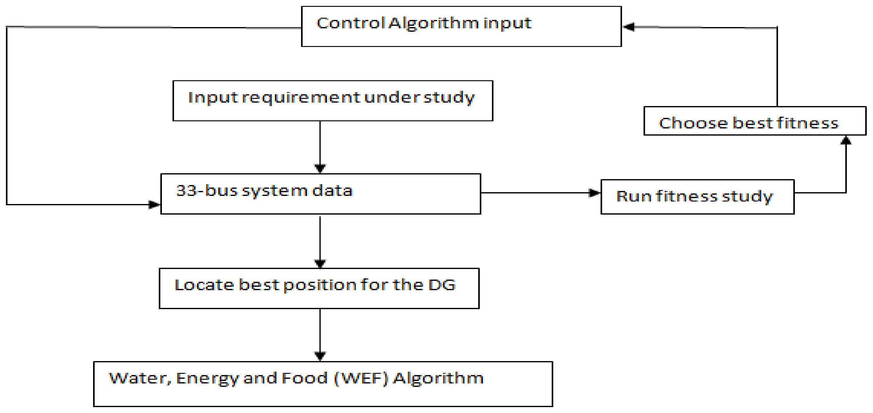
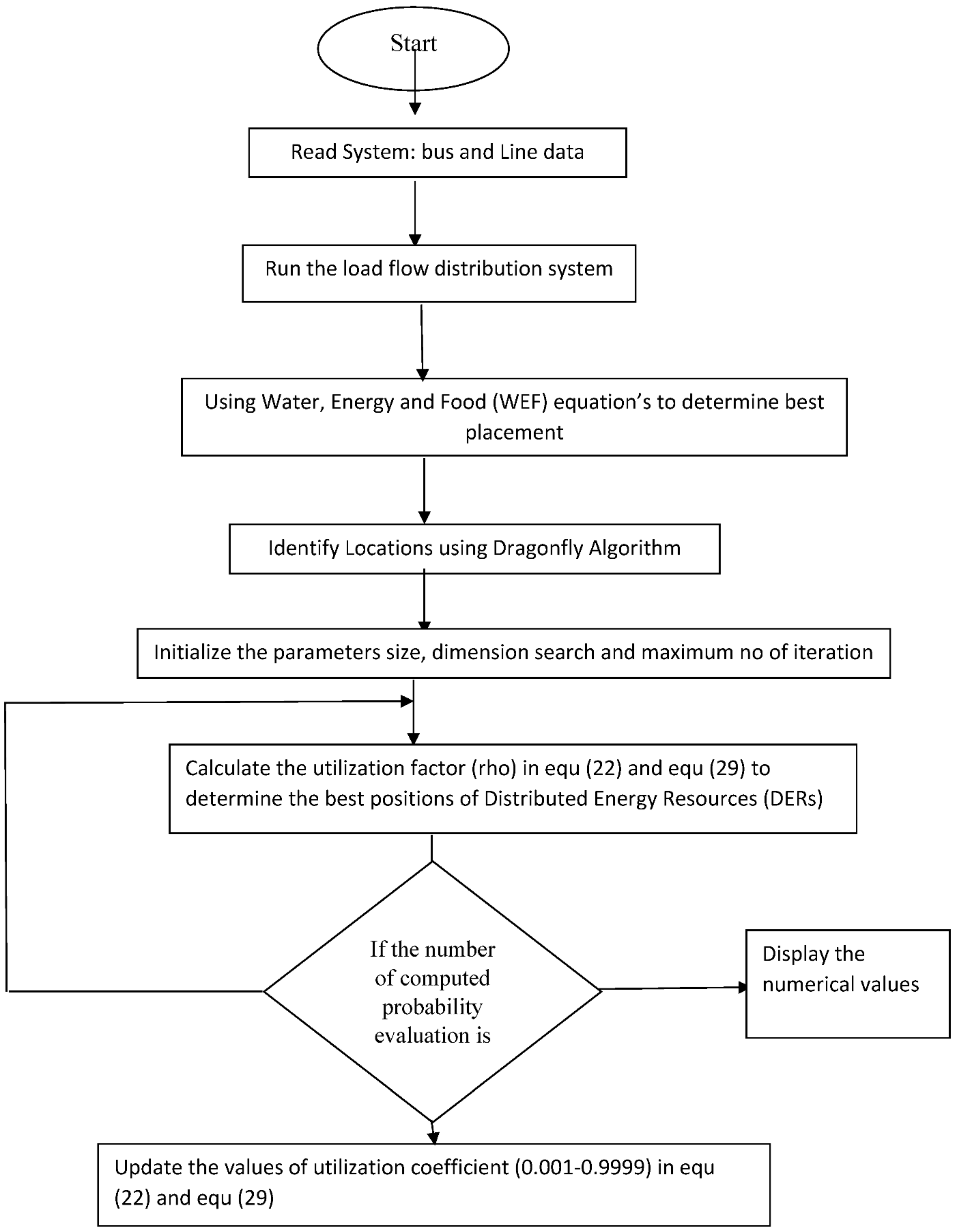
3.8. Flowchart for Configuration

WEF is used in the reconfiguration of the distribution system, and it decides the operation of the DG’s by providing eight (8) possible ways to position the DG in DN. However, this problem lies in two states of [0, 1]. The binary values of 0 and 1 signify the performance of the DG’S.

4. Numerical Simulations and Validation Approximations

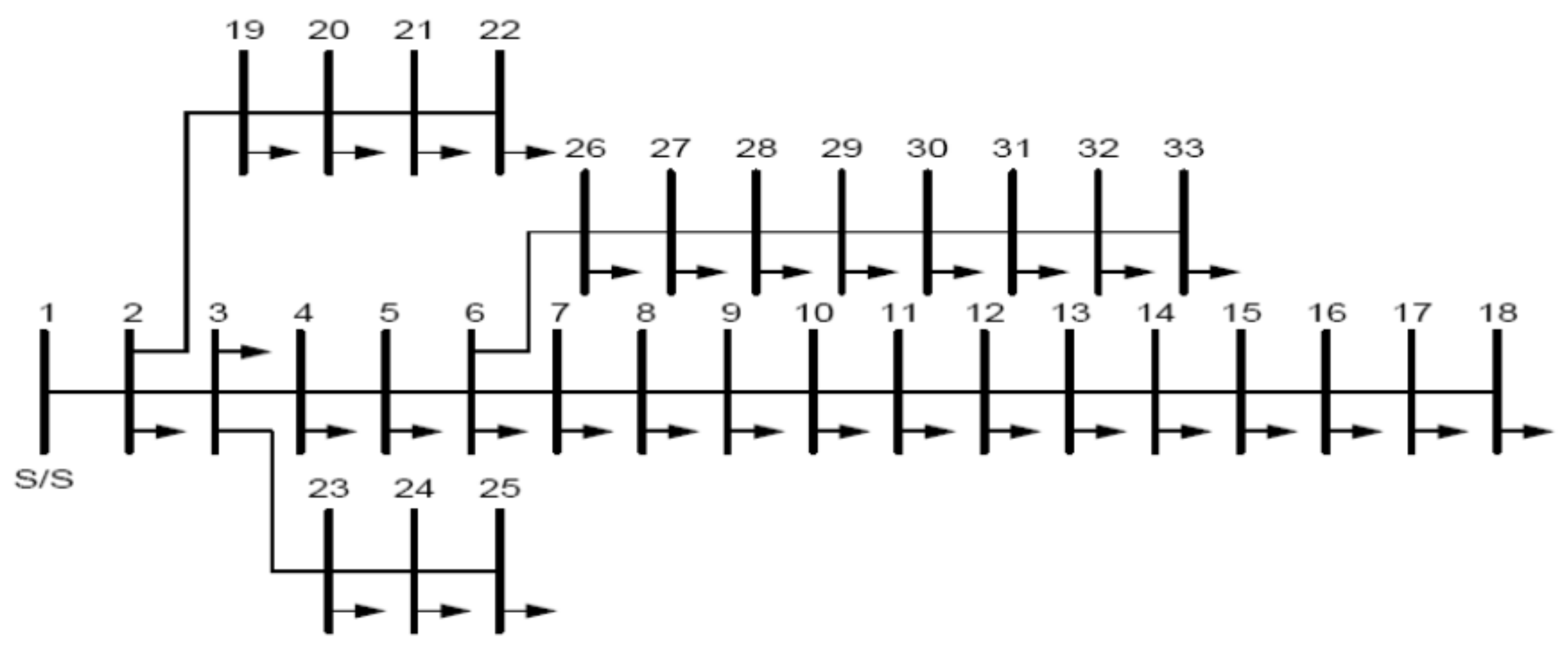
4.1. 33-Bus Test System

For numerical simulations and validation of the WEF Algorithm designed in this work. The optimal location of the Gas turbine, wind turbines, solar, and their settings is to optimize the objective function as discussed above. The objective function that was considered Cumulative voltage deviation (CVD), total power loss, overall efficiency, and total emissions produced by this conventional gas system and cost minimization of the energy sources. The proposed method is applied to the 33-bus system as shown figure below. The system is connected to the main substation of 132/12.66 KV and consists of 32 branches/lines and 33 buses with the size of load at 3.715 MW and 2.300 MVar. All these data of the line and buses are taken from [44], as shown in Figure 2. The block diagram for the optimal placement in IEEE 33 bus system with DG and Without DG is shown in Figure 3. The flowchart that handles the Algorithm selected for this work is given in Figure 4 below.

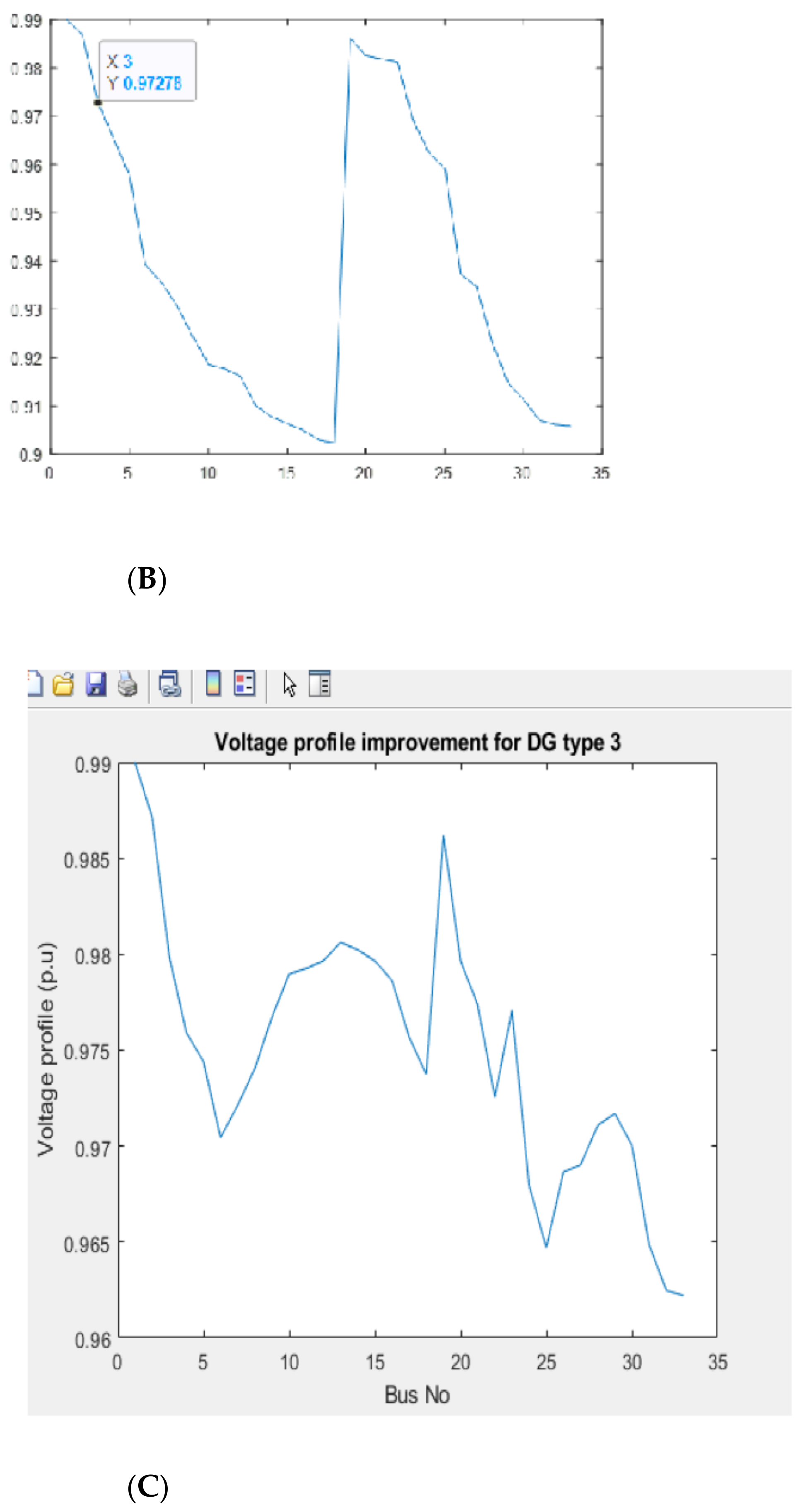
4.2. Results and Discussion

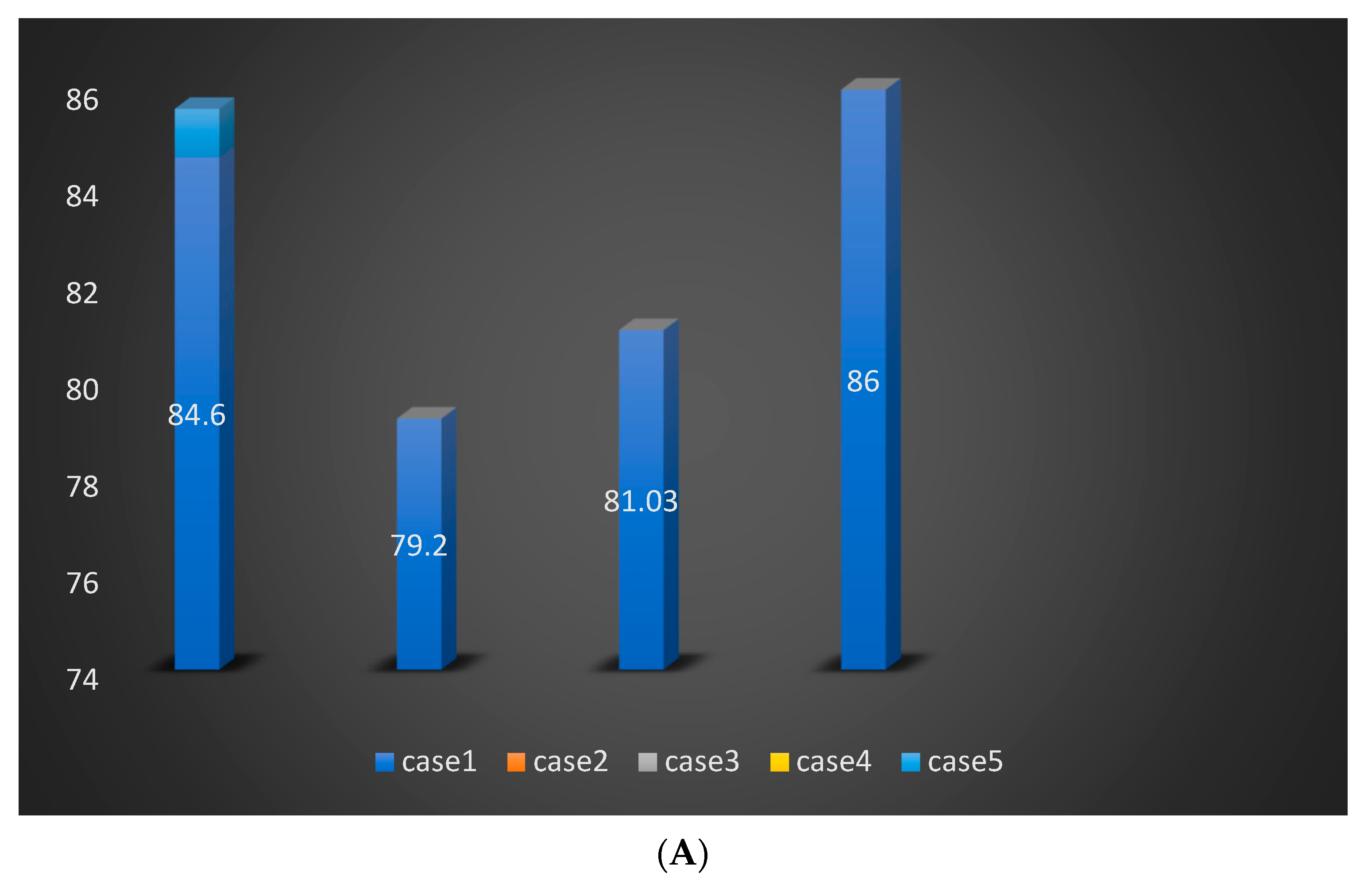
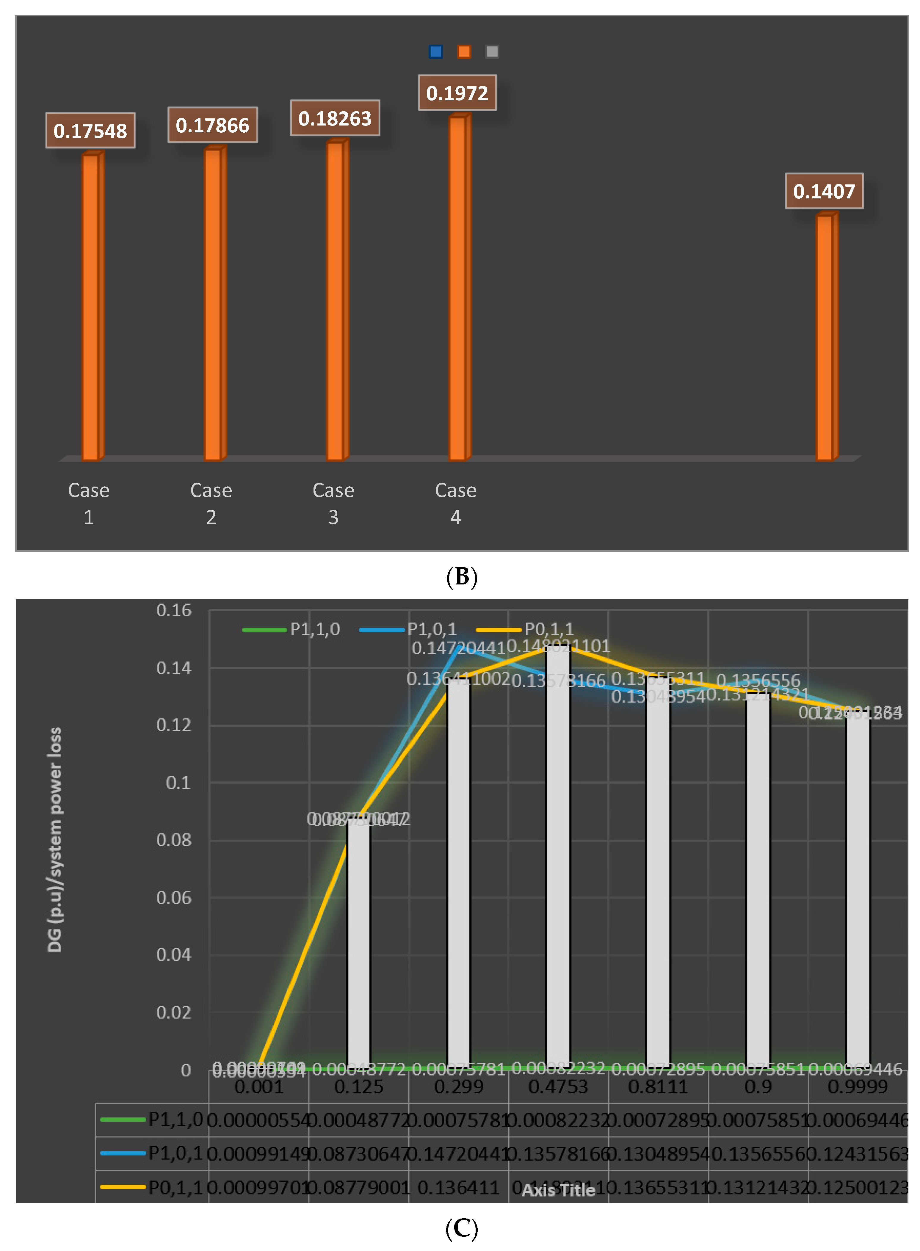
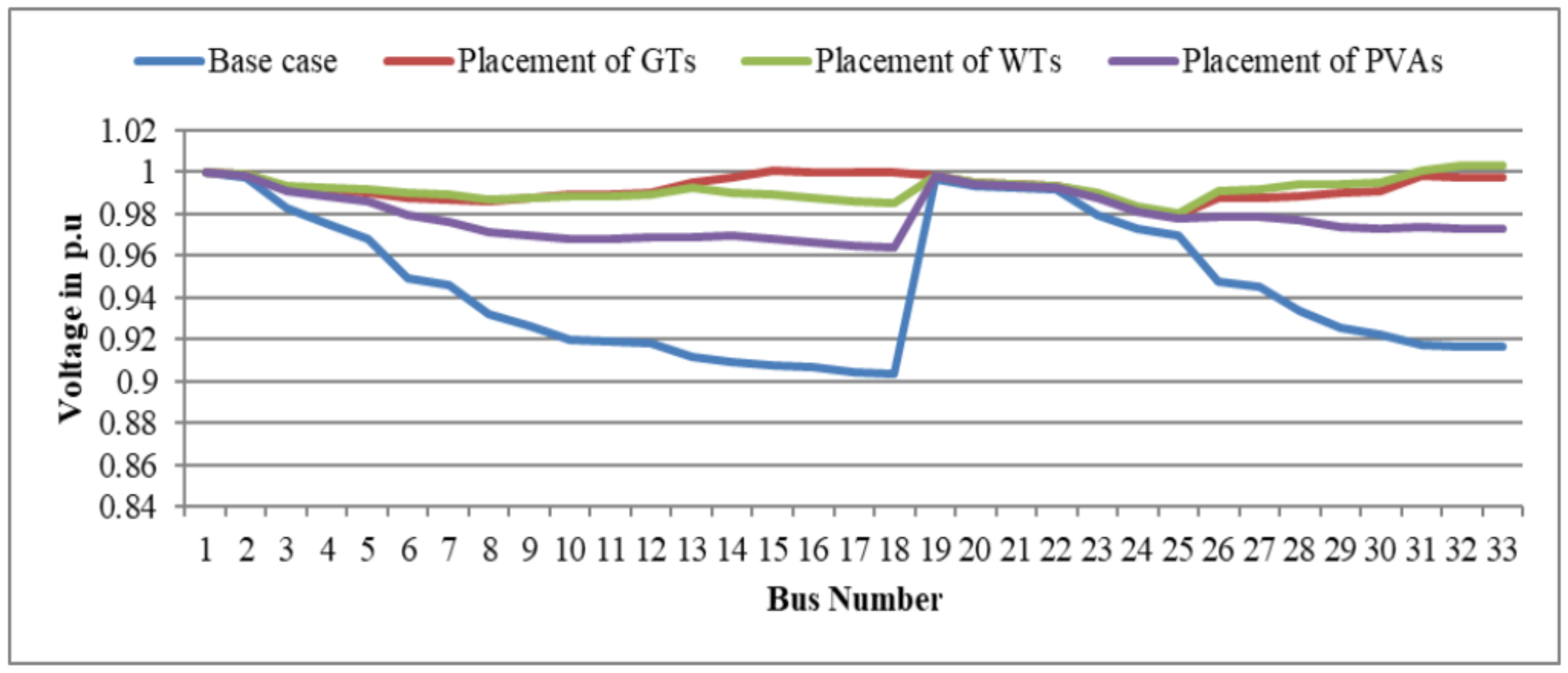
The major aim of this simulation is to locate three various DG with different sizes. The results obtained from the five (5) cases were summarized below in

Table 4. Result obtained for the case study.

	CASE1	CASE2	CASE3	CASE4	CASE5
DG CAPACITY IN (MW)	0.5, 0.65, 0.7	0.6, 0.63, 0.8	0.4, 0.5, 0.75	0.50, 0.55, 0.7	0.6, 0.63, 0.65
LOCATION OF BUS NUMBER	31, 15, 9	31, 9, 15	25, 16, 11	25, 11, 16	31, 16, 11
MAXMIUM POWER LOSS (KW)	84.60	79.20	81.03	86.0	85.4
VOLTAGE PROFILE IMPROVEMENT	0.17548	0.17866	0.18263	0.1972	0.1407
STABILITY INDEX	1.146	1.1345	1.156	1.1713	1.173
UTILIZATION RATE	3.9 × 10−6	0.0354	0.1256	0.4542	0.5635
EMISSION (IB/h)	2046.18	1160.23	2303.67	4606.44	320.65

and a comparison was carried out in

Table 5. Compares the results of the various methods for the test systems for the allocation of a single and multiple DG units.

Method	DG Location Bus Number/Bus Location	Voltage (p.u)	Power Loss (kW)
Genetic algorithm (GA) [45]	GA PSO 6 13 24 30 0.6429 0.8571 0.8571 0.7382	0.9703	0.0682
BFOA [46]	0.542 (17), 0.160 (18), 0.895 (33)	0.978	41.41
GA [47]	0.25 (16), 0.25 (22), 0.50 (30)	0.971	71.25
WEF Case 1, 2 and 3	31 15 9 0.50 0.65 0.70	0.9622 *	21.57 *

to show the effectiveness of the new Algorithm. The DG capacity for all cases was considered to range from a minimum value of 0.5 MW to a maximum value of 0.8. In the case of Algorithm 1, we have calculated the maximum DG capacity as 0.5, 0.65, and 0.70 by placing this DG at positions 31, 15, and 9. However, the best cases among all cases consider are case 2, which is having a value ranging from 0.60–0.80 in terms of losses and located at bus 31, 15, and 9. There is a strong significance in terms of voltage profile improvement.

In DG type one, from Table 1; Gas turbine usage is highly connected to solar usage at a low occupation rate. Similarly, the Gas turbine is connected to wind energy at a high occupation rate. It can be seen when $\rho \to 0.100 \mathrm{and} \rho \to 0.1250$, the rotational value for the algorithm does not show much difference between each other. This implies that there is a strong relationship between having Gas turbine DG and solar DG based at an idle state of operation in comparison to the other point.

In DG type two, occupying Gas turbine and Wind energy is similar to occupying Solar and wind DG position. This is evident from Table 2 above. One can see that if ρ approaches 0.999 from below, the values of $\rho \to 0.0010$ and $\rho \to 0.9999$ are approximately the same. Consequently, the busy periods of the two states’ DG are equivalent. At this stage we assume the allocation is at idle state and no losses will be recorded, hence placement is at the right position.

In DG type three, from the view of Table 3, there is a high rate of occupying all the best positions from the results obtained.

The parameters considered for DFA for both the test systems are number of search agents = 20, dimension of search space (d = 5), separation weight (s = 0.1), alignment weight (a = 0.1), cohesion weight (c = 0.7), food attraction weight (f = 1), enemy distraction weight (e = 1) and inertia weight (w = 0.9) and maximum number of iterations = 100.

Table 5 compares the results of the various methods for the test systems for the allocation of a single DG unit, two DG units, and three DG units. The comparison is carried out concerning the DG locations, DG sizes, and RPL. Table 5. Compares the values obtained from our test system (Matlab Simulation).

One can observe in the following as objective functions achieved in Figure 5A–C: (A) Result of objective function in terms of power loss reduction with installation of DG system. (B) Result of voltage profile improvement with installation of DG System. (C) DG size, bus location and system power loss of 33-bus test system.

The base case voltages for the allocation values in each bus are presented in Figure 6, the values of the voltages in (per units) are represented in the vertical axis, while the bus numbers are represented in horizontal axis. It can be observed from Figure 6.placement of hybrid renewable system based on the proposed methodology significantly reduces loses, which is expected as part of the technical objectives.

4.3. Power Losses

Table 6. Power loss comparison considering case study with DG and without DG.

	Active Power Loss
Base model without a Gas turbine, Wind DG and Solar PV	$\mathrm{Power} \mathrm{Loss}=2.067320\times {10}^2$$\mathrm{KW}, \mathrm{Power} \mathrm{Loss}=1.379097\times {10}^2$ KVAr
The base model with the Gas turbine, wind DG and Solar PV	$\mathrm{Power} \mathrm{Loss}=1.115737\times {10}^2 \mathrm{KW},$$\mathrm{Power} \mathrm{Loss}=7.293871\times {10}^1 \mathrm{KVAr}$ $\mathrm{DG}1 \mathrm{Power}=8.738701\times {10}^2$ $\mathrm{DG}2 \mathrm{power}=1.310805\times {10}^3$ $\mathrm{DG}3 \mathrm{Power}=8.738701\times {10}^2$

presents a comparison of real and reactive power losses before and after reconfiguration and DG placement in the distribution network. Losses minimized throughout the 1st, 2nd, and 3rd intervals are up to 21.57 when compared to that [48].

The behavior of our algorithm is captured in graphical form as shown in Figure 7A–C.

5. Conclusions

Most algorithms proposed in the literature by various authors to solve optimal DG placement problems consider only location and size as the variables of optimization in minimizing the power loss in a network. However, Renewable Distributed Generations technology also plays an important role in minimizing the loss of the power network. The new methodology proposed to optimally place the Gas turbine, wind DG and Solar PV to minimize the active power loss of the system using WEF has been fully discussed in this paper. Water, Energy, and Food algorithm, is easy to implement and the time taken for the iteration is less compared to other conventional methods and it is accurate. An efficient WEF is used in the optimization process of allocation DG in the distribution system. The developed algorithm successfully optimized the location and size (penetration level) of the DG and determines the appropriate DG technology. It was further shown that the algorithm was able to optimally locate and size more DGs to further reduce losses on the network. The results show that the optimal allocation of the Gas turbine, wind DG and Solar PV will minimize the real power loss as well as the reduction in emission as shown in Table 4, and it is tested on IEEE 33-bus system and shows improvement in the Results display minimization in losses up to 70% and remarkable improvement in voltage profile at every load bus.

References

1. Sulaiman, M.H.; Mustafa, M.W.; Azmi, A.; Aliman, O.; Abdul Rahim, S.R. Optimal allocation and sizing of distributed generation in distribution system via firefly algorithm. In Proceedings of the 2012 IEEE International Power Engineering and Optimization Conference (PEOCO2012), Melaka, Malaysia, 6–7 June 2012; pp. 84–89. [Google Scholar]
2. Chatterjee, S. An analytic method for allocation of Distributed Generation in radial distribution system. In Proceedings of the IEEE Indicon, New Delhi, India, 17–20 December 2015; pp. 4–8. [Google Scholar]
3. Huda, A.S.N.; Živanović, R. Large-scale integration of distributed generation into distribution networks: Study objectives, review of models and computational tools. Renew. Sustain. Energy Rev. 2017, 76, 974–988. [Google Scholar] [CrossRef]
4. Ehsan, A.; Yang, Q. Optimal integration and planning of renewable distributed generation in the power distribution networks: A review of analytical techniques. Appl. Energy 2018, 210, 44–59. [Google Scholar] [CrossRef]
5. Li, Y.; Feng, B.; Li, G.; Qi, J.; Zhao, D.; Mu, Y. Optimal distributed generation planning in active distribution networks considering integration of energy storage. Appl. Energy 2018, 210, 1073–1081. [Google Scholar] [CrossRef] [Green Version]
6. Sudabattula, S.; Kowsalya, M. Optimal Allocation of Wind Based Distributed Generators in Distribution System Using Cuckoo Search Algorithm. Procedia Comput. Sci. 2016, 92, 298–304. [Google Scholar] [CrossRef] [Green Version]
7. Rao, R.S.; Ravindra, K.; Satish, K.; Narasimham, S.V.L. Power loss minimization in distribution system using network reconfiguration in the presence of distributed generation. IEEE Trans. Power Syst. 2013, 28, 317–325. [Google Scholar] [CrossRef]
8. Georgilakis, P.S.; Hatziargyriou, N.D. In Power Distribution Networks: Models, Methods, and Future Research. IEEE Trans. Power Syst. 2013, 28, 3420–3428. [Google Scholar] [CrossRef]
9. Acharya, N.; Mahat, P.; Mithulananthan, N. An analytical approach for DG allocation in primary distribution network. Int. J. Electr. Power Energy Syst. 2006, 28, 669–678. [Google Scholar] [CrossRef]
10. Wang, C.; Nehrir, M.H. Analytical approaches for optimal placement of distributed generation sources in power systems. IEEE Trans. Power Syst. 2004, 19, 2068–2076. [Google Scholar] [CrossRef]
11. Gözel, T.; Hocaoglu, M.H. An analytical method for the sizing and siting of distributed generators in radial systems. Electr. Power Syst. Res. 2009, 79, 912–918. [Google Scholar] [CrossRef]
12. Hung, D.Q.; Mithulananthan, N.; Bansal, R.C. Analytical expressions for DG allocation in primary distribution networks. IEEE Trans. Energy Convers. 2010, 25, 814–820. [Google Scholar] [CrossRef]
13. Moradi, M.H.; Abedini, M. A combination of genetic algorithm and particle swarm optimization for optimal distributed generation location and sizing in distribution systems with fuzzy optimal theory. Int. J. Green Energy 2012, 9, 641–660. [Google Scholar] [CrossRef]
14. El-Zonkoly, A.M. Optimal placement of multi-distributed generation units including different load models using particle swarm optimization. Swarm Evol. Comput. 2011, 1, 50–59. [Google Scholar] [CrossRef]
15. Jain, N.; Singh, S.N.; Srivastava, S.C. A generalized approach for DG planning and viability analysis under market scenario. IEEE Trans. Ind. Electron. 2013, 60, 5075–5085. [Google Scholar] [CrossRef]
16. Abu-Mouti, F.S.; El-Hawary, M.E. Optimal distributed generation allocation and sizing in distribution systems via artificial bee colony algorithm. IEEE Trans. Power Deliv. 2011, 26, 2090–2101. [Google Scholar] [CrossRef]
17. Tolba, M.A.; Tulsky, V.N.; Diab, A.A.Z. Optimal Allocation and Sizing of Multiple Distributed Generators in Distribution Networks Using a Novel Hybrid Particle Swarm Optimization Algorithm. In Proceedings of the 2017 IEEE Conference of Russian Young Researchers in Electrical and Electronic Engineering (EIConRus), St. Petersburg/Moscow, Russia, 1–3 February 2017; pp. 1606–1612. [Google Scholar]
18. Parizad, A.; Khazali, A.H.; Kalantar, M. Sitting and sizing of distributed generation through Harmony Search Algorithm for improve voltage profile and reducuction of THD and losses. In Proceedings of the Canadian Conference on Electrical and Computer Engineering (CCECE) 2010, Calgary, AB, Canada, 16 September 2010. [Google Scholar]
19. Khalesi, N.; Rezaei, N.; Haghifam, M.R. DG allocation with application of dynamic programming for loss reduction and reliability improvement. Int. J. Electr. Power Energy Syst. 2011, 33, 288–295. [Google Scholar] [CrossRef]
20. Kumar, S.; Kumar, N.P. Electrical Power and Energy Systems A novel approach to identify optimal access point and capacity of multiple DGs in a small, medium and large scale radial distribution systems. Int. J. Electr. Power Energy Syst. 2013, 45, 142–151. [Google Scholar]
21. Zhang, H.; Vittal, V.; Heydt, G.T.; Quintero, J. A mixed-integer linear programming approach for multi-stage security-constrained transmission expansion planning. IEEE Trans. Power Syst. 2012, 27, 1125–1133. [Google Scholar] [CrossRef]
22. Hung, D.Q.; Mithulananthan, N. Multiple distributed generator placement in primary distribution networks for loss reduction. IEEE Trans. Ind. Electron. 2013, 60, 1700–1708. [Google Scholar] [CrossRef]
23. Yuvaraj, T.; Devabalaji, K.R.; Ravi, K. Optimal Placement and Sizing of DSTATCOM Using Harmony Search Algorithm; Elsevier B.V.: Amsterdam, The Netherlands, 2015; Volume 79, ISBN 1876-6102. [Google Scholar]
24. Murthy, V.V.S.N.; Kumar, A. Comparison of optimal DG allocation methods in radial distribution systems based on sensitivity approaches. Int. J. Electr. Power Energy Syst. 2013, 53, 450–467. [Google Scholar] [CrossRef]
25. Tan, W.S.; Hassan, M.Y.; Rahman, H.A.; Abdullah, P. Multi-distributed generation planning using hybrid particle swarm optimisation-gravitational search algorithm including voltage rise issue. IET Gener. Transm. Distrib. 2013, 7, 929–942. [Google Scholar] [CrossRef]
26. Mahmoud, G.A.E.-A.; Oda, E.S.S. Investigation of Connecting Wind Turbine to Radial Distribution System on Voltage Stability Using SI Index and λ-v Curves. Smart Grid Renew. Energy 2016, 7, 16–45. [Google Scholar] [CrossRef] [Green Version]
27. Hanumantha Rao, B.; Sivanagaraju, S. Optimum allocation and sizing of distributed generations based on clonal selection algorithm for loss reduction and technical benefit of energy savings. In Proceedings of the 2012 International Conference on Advances in Power Conversion and Energy Technologies (APCET), Mylavaram, Andhra Pradesh, 2–4 August 2012; pp. 1–5. [Google Scholar]
28. Abdelsalam, A.A.; Zidan, A.A.; El-Saadany, E.F. Optimal DG Allocation in Radial Distribution Systems with High Penetration of Non-linear Loads. Electr. Power Compon. Syst. 2015, 43, 1487–1497. [Google Scholar] [CrossRef]
29. Bin Muhtazaruddin, M.N.; Fujita, G. Distribution network power loss by using Artificial Bee Colony. In Proceedings of the 2013 48th International Universities’ Power Engineering Conference (UPEC), Dublin, Ireland, 2–5 September 2013. [Google Scholar]
30. Hegazy, Y.G.; Othman, M.M.; El-Khattam, W.; Abdelaziz, A.Y. Optimal sizing and siting of distributed generators using Big Bang Big Crunch method. In Proceedings of the 2014 49th International Universities Power Engineering Conference (UPEC), Cluj-Napoca, Romania, 2–5 September 2014; pp. 1–6. [Google Scholar]
31. El-Fergany, A. Study impact of various load models on DG placement and sizing using backtracking search algorithm. Appl. Soft Comput. J. 2015, 30, 803–811. [Google Scholar] [CrossRef]
32. Sani, S.; Shuaibu, A.; Tumushabe, A.; Mbatudde, M. Modeling the Water-Energy-Food Nexus in ObR-E’s: The Eight (8) Coordinates. Appl. Appl. Math. Int. J. 2019, 14, 27. [Google Scholar]
33. Jin, L.; Chang, Y.; Ju, X.; Xu, F. A Study on the Sustainable Development of Water, Energy, and Food in China. Int. J. Environ. Res. Public Health Artic. 2019, 16, 3688. [Google Scholar] [CrossRef] [Green Version]
34. Diamond, J. Collapse: How Societies Choose to Fail or Succeed. ISBN 0670033375. Wikipedia. United States. 2005. Available online: https://en.wikipedia.org/wiki/Collapse:_How_Societies_Choose_to_Fail_or_Succeed (accessed on 20 February 2022).
35. Al-saidi, M.; Elagib, N.A. Science of the Total Environment Towards understanding the integrative approach of the water, energy and food nexus. Sci. Total Environ. 2017, 574, 1131–1139. [Google Scholar] [CrossRef]
36. Mirjalili, S. Dragonfly algorithm: A new meta-heuristic optimization technique for solving single-objective, discrete, and multi-objective problems. Neural Comput. Appl. 2016, 27, 1053–1073. [Google Scholar] [CrossRef]
37. Oda, E.S.; Abdelsalam, A.A.; Abdel-Wahab, M.N.; El-Saadawi, M.M. Distributed generations planning using flower pollination algorithm for enhancing distribution system voltage stability. Ain Shams Eng. J. 2017, 8, 593–603. [Google Scholar] [CrossRef] [Green Version]
38. Ekpa, T.K.; Sani, S.; Hassan, A.S.; Kalyankolo, Z. On Improving Power Supply Flexibility. J. Niger. Assoc. Math. Phys. 2018, 48, 347–352. [Google Scholar]
39. Sanjay, R.; Jayabarathi, T.; Raghunathan, T.; Ramesh, V.; Mithulananthan, N. Optimal allocation of distributed generation using hybrid grey Wolf optimizer. IEEE Access 2017, 5, 14807–14818. [Google Scholar] [CrossRef]
40. Sarkar, A.; Behera, D.K. Wind Turbine Blade Efficiency and Power Calculation with Electrical Analogy. Int. J. Sci. Res. Publ. 2012, 2, 2250–3153. [Google Scholar]
41. Bawazir, R.O.; Cetin, N.S. Comprehensive overview of optimizing PV-DG allocation in power system and solar energy resource potential assessments. Energy Rep. 2020, 6, 173–208. [Google Scholar] [CrossRef]
42. Hassan, A.S.; Sun, Y.; Wang, Z. Optimization techniques applied for optimal planning and integration of renewable energy sources based on distributed generation: Recent trends Optimization techniques applied for optimal planning and integration of renewable energy sources based on distributed generation: Recent trends. Cogent Eng. 2020, 7, 1766394. [Google Scholar]
43. Singh, A.K.; Parida, S.K. Combined Optimal Placement of Solar, Wind and Fuel cell Based DGs Using AHP. In Proceedings of the World Renewable Energy Congress-Sweden, Linköping, Sweden, 8–13 May 2011; Linköping University Electronic Press: Johor Bahru, Malaysia; pp. 3113–3120. [Google Scholar]
44. Kashem, M.A.; Ganapathy, V.; Jasmon, G.B.; Buhari, M.I. A Novel Method for Loss Minimization in Distribution Networks. In Proceedings of the International Conference on Electric Utility Deregulation and Restructuring and Power Technologies, London, UK, 4–7 April 2000. [Google Scholar]
45. Moradi, M.H.; Abedini, M. A Combination of Genetic Algorithm and Particle Swarm Optimization for Optimal DG location and Sizing in Distribution Systems. Int. J. Electr. Power Energy Syst. 2012, 34, 66–74. [Google Scholar] [CrossRef]
46. Imran, M. Optimal Distributed Generation and Capacitor placement in Power Distribution Networks for Power Loss Minimization. In Proceedings of the 2014 International Conference on Advances in Electrical Engineering (ICAEE), Vellore, India, 9–11 January 2014. [Google Scholar]
47. Saonerkar, A.K.; Bagde, B.Y. Optimized DG placement in radial distribution system with reconfiguration and capacitor placement using genetic algorithm. In Proceedings of the 2014 IEEE International Conference on Advanced Communication Control and Computing Technologies (TCACCCT), Ramanathapuram, India, 8–10 May 2014; pp. 1077–1083. [Google Scholar]
48. Esmaeilian, H.R.; Fadaeinedjad, R. Energy Loss Minimization in Distribution Systems Utilizing an Enhanced Reconfiguration Method Integrating Distributed Generation. IEEE Syst. J. 2015, 9, 1430–1439. [Google Scholar] [CrossRef]
Figure 1. Single line diagram of a feeder [39].
Energies 15 02242 g001
Figure 2. A case study of the 33-bus system under study [45].
Energies 15 02242 g002
Figure 3. Block diagram for allocation of DG.
Energies 15 02242 g003
Figure 4. Optimal DG allocation methodology.
Energies 15 02242 g004
Figure 5. (A) Result of objective function in terms of power loss reduction with installation of DG system. (B) Result of voltage profile improvement with installation of DG System. (C) DG size, bus location and system power loss of 33-bus test system.
Energies 15 02242 g005aEnergies 15 02242 g005b
Figure 6. Voltage profile of 33 bus test system with optimal allocation of GTs, WTs, and PVAs placed in DS.
Energies 15 02242 g006
Figure 7. (A) Voltage profile of 33 bus test system without DG; (B) Voltage profile 33-bus system considering placement of DG’s type two; (C): Voltage profile 33-bus system considering placement of DGs type three.
Energies 15 02242 g007aEnergies 15 02242 g007b