An Hour-Ahead PV Power Forecasting Method Based on an RNN-LSTM Model for Three Different PV Plants

Abstract

Incorporating solar energy into a grid necessitates an accurate power production forecast for photovoltaic (PV) facilities. In this research, output PV power was predicted at an hour ahead on yearly basis for three different PV plants based on polycrystalline (p-si), monocrystalline (m-si), and thin-film (a-si) technologies over a four-year period. Wind speed, module temperature, ambiance, and solar irradiation were among the input characteristics taken into account. Each PV plant power output was the output parameter. A deep learning method (RNN-LSTM) was developed and evaluated against existing techniques to forecast the PV output power of the selected PV plant. The proposed technique was compared with regression (GPR, GPR (PCA)), hybrid ANFIS (grid partitioning, subtractive clustering and FCM) and machine learning (ANN, SVR, SVR (PCA)) methods. Furthermore, different LSTM structures were also investigated, with recurrent neural networks (RNN) based on 2019 data to determine the best structure. The following parameters of prediction accuracy measure were considered: RMSE, MSE, MAE, correlation (r) and determination (R²) coefficients. In comparison to all other approaches, RNN-LSTM had higher prediction accuracy on the basis of minimum (RMSE and MSE) and maximum (r and R²). The p-si, m-si and a-si PV plants showed the lowest RMSE values of 26.85 W/m², 19.78 W/m² and 39.2 W/m² respectively. Moreover, the proposed method was found to be robust and flexible in forecasting the output power of the three considered different photovoltaic plants.

1. Introduction

Globalization and the economic growth of the world have triggered an increase in the need for electrical energy, and the principal sources of electrical energy are fossil fuels. Oil, coal and gas reserves have an approximate life of 35, 107, and 37 years, respectively [1]. Huge emissions of gases such as CO₂ and greenhouse gas (GHG) as a result of the massive use of fossil fuels is polluting the environment, leading to world climate change [2]. In light of these facts, PV energy has attained significant importance among other renewable energy sources. Power generation from PV sources has a major impact on the environment, with no GHG emissions [3,4], long life, and low maintenance costs compared to typical energy sources [5,6,7,8]. However, natural fluctuations of solar radiation and temperature affect PV output power, reducing the reliability, stability, and planning of power grids. To keep the balance between energy supply and power system demand [9], the variable properties of PV energy are applied to both sides of the power grid to control PV power absorption [10,11]. The forecasting of output PV power is therefore crucially important to improve power absorption.

In general, forecasting is performed based on different time periods known as forecasting horizons. Very short-term forecasting (1 s ≤ 1 h) helps with real-time electricity distribution, resource optimization, and power leveling [12]. Short-term forecasting (1 h–24 h) helps to enhance grid reliability and improvise power system operations [13]. Medium term forecasting (one week–one month) establishes the schedule for the planning and maintenance of power systems by forecasting existing electric power. Long-term forecasting (one month–one year) incorporates distribution and transmission governing bodies, the planning of electricity generation, and energy bidding and security actions [14,15].

Various techniques have been used to forecast PV power output, such as ARMA, ARIMA, ARMAX, coupled autoregressive and dynamic systems (CARDS), regression, and regression trees. The forecasting accuracy of these techniques is better for short-term horizons. However, accuracy declines with rising forecast horizon and output dimensions [16,17,18,19]. Non-linear data are also a limitation of these methods. Based on cloud tracking and prediction, sky and satellite photos were utilized to predict solar irradiance on an ultra-short-term basis [20,21,22]. The forecasting accuracy of image-based methods is directly dependent on image processing algorithms. However, based on low-resolution satellite data and limited coverage of sky images from the ground, the forecasting accuracy of these methods needs further improvement. Numerical weather prediction (NWP) is used for medium-term (15 days ahead) solar irradiance forecasting. However, its application is limited because of data retrieval restrictions imposed by domestic meteorological departments [23,24,25,26].

An artificial neural network (ANN) in [27,28,29,30] and an adaptive neuro-fuzzy inference system (ANFIS) in [31] are among the machine learning methods deployed for solar power forecasting. These are better able to deal with non-linear systems and cope with the variable behavior of solar power. However, issues of random initial data, local minima, overfitting, and increased complexity because of multilayered structure affect the reliability of power systems [6,32,33]. Support vector machines (SVM), meanwhile, show better forecast accuracy for predicting solar power in [34,35,36]. However, these are extremely susceptible to parameters such as penalty factor (C), kernel function and the tube radius (ɛ). Making an appropriate choice for these parameters is therefore a difficult task [5]. The weights and biases of buried nodes in an extreme learning machine (ELM) are chosen at random [37,38,39].

New advances in artificial intelligence (AI) technology have led to the use of various deep learning techniques in certain fields to overcome the shortcomings of traditional neural networks and other machine learning techniques [40,41]. Deep learning has the following major traits in contrast with physical, persistence and statistical methods [42]: unsupervised feature extraction, dominant generalization ability, and training on big data.

K Wang developed a model based on the combination of CNN and LSTM for the day-ahead solar power output forecasting, showing better forecasting accuracy than individual methods, with the increase in the input sequence [43]. A physical constrained LSTM model (PC-LSTM) has shown better hour-ahead solar power forecasting accuracy than statistical and conventional machine learning models [44]. The Deep Belief network [45] based on the proposed gray theory to predict the output power of a solar system for a day ahead showed better prediction accuracy and computational efficiency. Wang et al. [2] developed a temporal correlation correction method to enhance the deep learning method accuracy for day-ahead solar power prediction. Navaez et al. presented day- and week-ahead PV power predictions using the deep learning method [42]. Using the local data, the LSTM method was developed to predict the output power for the next 24 h [46]. The forecasting accuracy of this method is 18.34% better than other benchmark methods. Very short-term power output forecasting for five minutes ahead has been executed for different PV technologies using actual field measurements [47]. However, all these studies lack deep learning-based PV power predictions for various PV power plants to ensure model robustness. According to the authors’ knowledge, comparison of the deep learning method with regression, neural networks, machine learning, and hybrid (ANFIS) methods combined is also missing. Therefore, it is still possible to develop a deep learning method to predict the output power of a PV plant over a four-year timeframe.

The purpose of this study was to create a deep learning method (RNN-LSTM) for predicting the power output of PV modules on yearly basis during the data collection period (2016–2019) of PV power plants based on p-si, m-si, and a-si technologies. Secondly, to compare the efficiency of the proposed method for hour-ahead forecasting of output power, we used ANN, SVR, GPR, SVR(PCA), GPR (PCA), and ANFIS (grid partitioning, subtractive clustering and FCM). Finally, an LSTM structure comparison was performed to choose the best LSTM structure. The following are the study’s primary contributions:

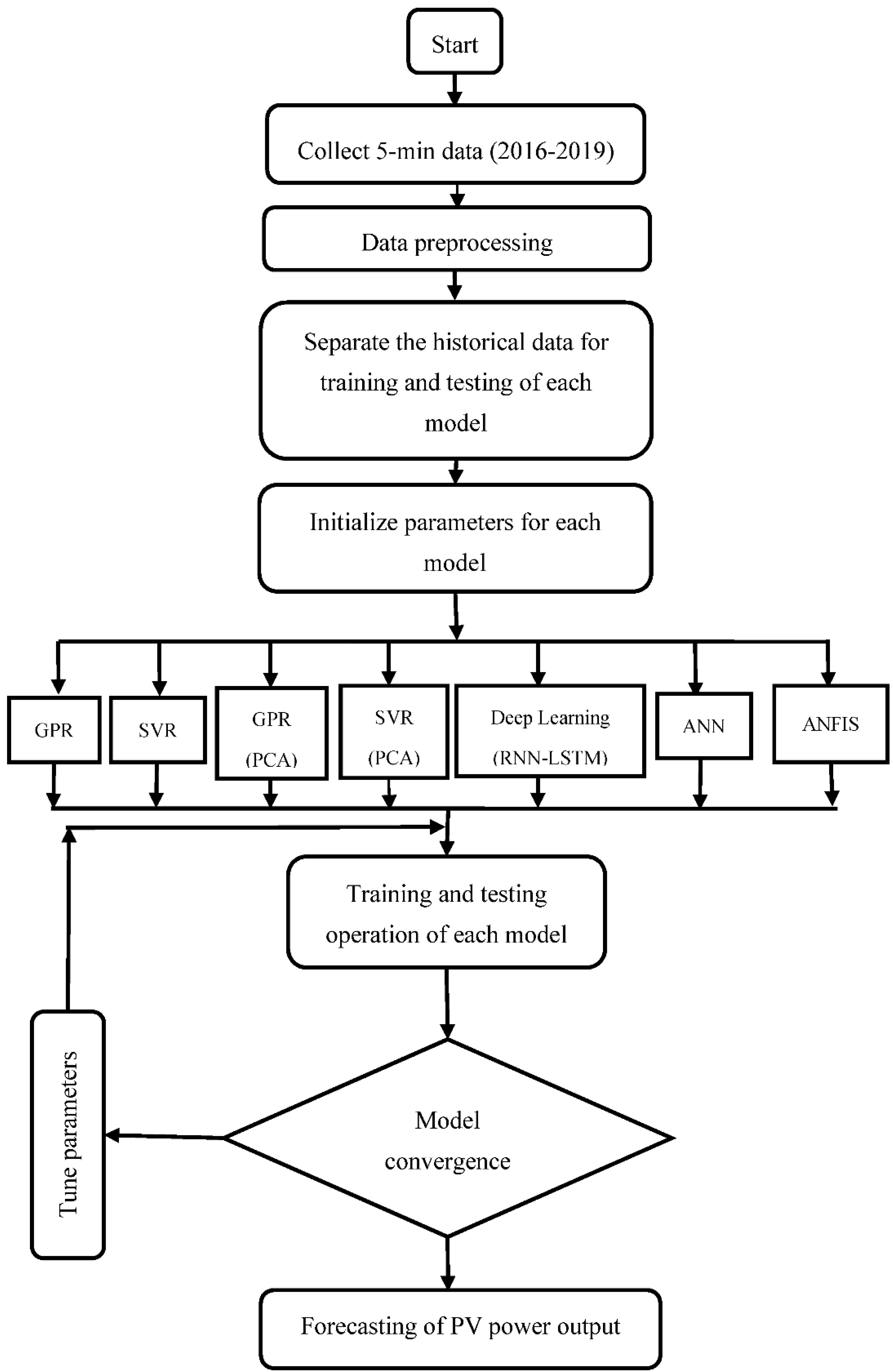
• Data preprocessing is performed for three different plants over the four years recording actual PV data.
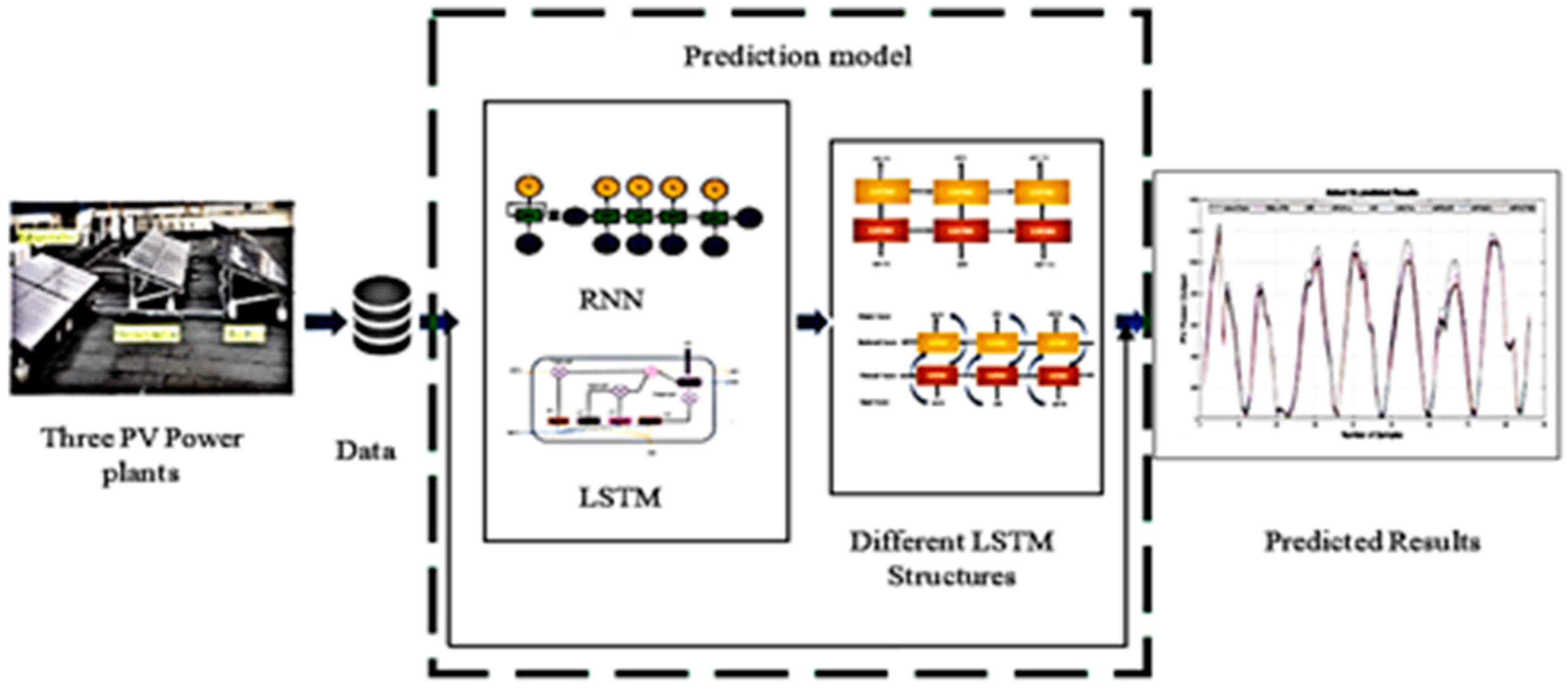
• A deep learning algorithm (RNN-LSTM) is proposed for hour-ahead forecasting of output PV power for three independent PV plants on yearly basis for a four-year period.
• Annual hour-ahead forecasting of PV output power using SVR, SVR(PCA), GPR, GPR (PCA), ANN, and ANFIS is also performed and compared with the proposed technique (RNN-LSTM) for the considered period (2016–2019).
• Different LSTM structures are also investigated with RNN to determine the most feasible structure, based on 2019 data only.

The rest of the paper is organized as follows. Section 2 delves into the approach in depth, while Section 3 and Section 4 offer the results and discussion, respectively. Finally, Section 5 presents the conclusions.

2. Methodology

Figure 1 depicts the suggested methodology’s research framework. This research investigates the performance of proposed deep learning and several prediction models on three different PV plants.

2.1. PV Plants Description and Data Set

Three types of PV plants were employed in this study: polycrystalline (p-si), monocrystalline (m-si), and thin-film (a-si), all of which were installed at the University of Malaya. The geographic position of the plants was 3°7′6″ North and 101°39′19″ East. There were 16 modules (125 W each) for p-si, 20 modules (75 W each) for m-si, and 20 modules (135 each) for the a-si PV system. For p-si, m-si, and a-si PV plants, the installed capacities were 2 KW, 1.875 KW, and 2.7 KW, respectively.

The forecasting performance was evaluated using data from the previous four years (2016–2019). Except for few days in 2018, the whole real data was properly synchronized and retrieved using a pyranometer for solar radiation, an anemometer for wind speed, and a temperature sensor to measure the temperature of the modules and environment. The missing data in 2018 were due to power failure of the sensors. These data were reinstated by acquiring the data of a similar date from the previous or next year. The data were recorded at a five-minute resolution on the web server.

The three PV power outputs (one for each PV) were collected using SMA SUNNY SENSOR BOX. Three variables (solar radiation, module temperature, and ambient temperature) typically have better correlation with the power output of PV plants. Wind speed in Malaysia is low due to tropical weather conditions, and therefore it has a very negligible effect on solar radiation. However, the correlation of the wind speed with the solar power output of each PV plant was found to be relatively better but inferior to the other three variables. Therefore, all four variables were considered as an input of each prediction model. Wind speed data have also been considered by other researchers for solar power output prediction [38,48]. Further details related to used sensors, inverters, and PV plants can be found in [49].

2.2. Data Preprocessing

Data preprocessing involves collection, division, and standardization of data. A database recorded over four years (2016–2019) was used in this research; 70% of each year of data was used for training, and the remaining 30% was utilized for testing purposes. The following formulae were used to normalize the data:

$$\mathsf{\mu }=\frac{1}{\mathrm{N}}{\displaystyle \sum }_{\mathrm{n}=1}^{\mathrm{N}}D$$

(1)

$$\mathsf{\sigma }=\mathrm{std}\left(D\right)$$

(2)

$$D_{Standardized}=\left(D-\mathsf{\mu }\right)/\mathsf{\sigma }$$

(3)

$$Y_{Predicted}=\sigma ·D_{Standardized}+\mathsf{\mu }$$

(4)

where μ represents the mean and σ stands for standard deviation of considered data (D). Equation (3) is used to normalize the data before it is trained, and Equation (4) is used to analyze the network testing performance by predicting the actual data. Figure 2 depicts the entire methodology’s flow chart.

2.3. Regression for PV Power Output Prediction

GPR and SVR are two regression algorithms used for the hour-ahead forecasting power output of PVs. These techniques were utilized by incorporating the principal component analysis (PCA) method. A 5-fold cross validation procedure was also adopted to justify the integrity of both forecasting methods. This procedure enabled the models to work properly by protecting them from overfitting and underfitting.

2.3.1. Gaussian Process Regression

This is a probabilistic non-parametric method which consists of kernel functions. It illustrates that a finite set of values follow the joint Gaussian distribution [50]. The GP model shows a path that indicates prior function distributions. For the training data D $=\left\{x_n,y_n\right\},$ where the input is $x_n$∈ ${ℝ}^{dx}$ and the output is $y_n$∈ R. Assume the following observation model:

$$y=f\left(x\right)+\mathrm{\varepsilon }$$

(5)

where f and $\mathrm{\varepsilon }$ are latent functions and Gaussian noise, respectively. The noise variance is ${\sigma }_n^2$, i.e., $\mathrm{\varepsilon }\sim \mathrm{N}\left(0,{\sigma }_n^2\right)$, while $y$ is the actual target value $y-{\left[y_1.........y_n\right]}^T$ and x is the input features as $x-{\left[x_1.........x_n\right]}^T$. P is the total number of new complete data sets. The prediction for the new sample $X_{test}$ is the average of all model predictions.

$$y_{predicted}=\frac{1}{P}{\displaystyle \sum }_{P=1}^P{M}_p\left(X_{test}\right)$$

(6)

where $M_p\left(X_{test}\right)$ represents the new test data set’s prediction result. In this study, the kernel function used for regression is Matern 5/2 and basis function is constant. The kernel scale, signal standard deviation, and sigma values are automatic.

2.3.2. Support Vector Regression (SVR)

Both regression and classification issues are solved using the SVM. It is utilized to improve generalization by lowering the empirical risk and confidence interval utilizing the structural risk minimization hypothesis. SVM can be used to solve regression problems, known as support vector regression (SVR), in addition to classification. For a data set of $\left\{\left(x_n,y_n\right)\frac{N}{n}=1\right\}$where $x_n$ and $y_n$ are the input and output vectors, while $N$ is the complete data set, SVM’s general mathematical function is as follows [51]:

$$y=f\left(x\right)={\displaystyle \sum }_{n=1}^M{\propto }_n·\phi \left(x\right)=w\phi \left(x\right)$$

(7)

$\phi \left(x\right)$ performs the nonlinear transformation, and the result is the linearly weighted sum of M. SVM’s decision function is as follows:

$$y=f\left(x\right)=\{{\displaystyle \sum }_{n=1}^N{\propto }_n·k(x_n,x)\}-b$$

(8)

The kernel function is denoted by the letter k. The kernel function must be chosen carefully to spread the data in a feature space. The bias values, objective function parameter, and training data are represented by $b$, ${\propto }_n$ and $N$, respectively, while the independent vectors and the vectors used in training are represented by $x$ and $x_n$. In this study, different kernel functions were experienced for SVM, namely: linear, Gaussian, coarse Gaussian, medium Gaussian, and quadratic. More accurate results were obtained with the cubic kernel function. The objective function parameter was RMSE. The kernel scale, box constraint and epsilon were automatic. The cubic SVM was tuned properly.

2.3.3. Principal Component Analysis (PCA)

The main component splits the collection of connected variables into smaller sets with no correlation, preserving the majority of the original data. Let W represent the input data set, which includes ambient and PV module temperature as well as solar irradiance and wind speed. Each column represents the sequence of n dimensional input [52]. The average of each function in the data set is considered zero $E\left(W\right)=0$. The original data matrix is represented with m samples and n variables as follows:

$$W={\left[w_1, w_2,\dots \dots .w_m\right]}^T=\left(\begin{array}{ccc}{w}_{11}& \dots & w_{1n}\\ ⋮& \ddots & ⋮\\ w_{m1}& \cdots & w_{mn}\end{array}\right)$$

(9)

The related eigenvectors show the new orthogonal components known as principal components while the matching eigenvalues define the magnitude of these principal components. The first principal component shows higher covariance when all the eigenvectors and eigenvalues are arranged in descending order. It should be noted that, despite the fact that the input variables are linked due to the orthogonality of the decomposed eigen vectors, there is no correlation between the resultant main components [53].

2.4. Artificial Neural Network (ANN) for PV Power Output Prediction

The ANN is a statistical model dealing with non-linear data properly. It has three layers: input, hidden, and output. The input layer displays information about inputs before the hidden layer analyzes it, while the hidden layer has a number of layers. After obtaining analyzed information from the hidden layer, the output layer describes the output. The ANN model can be represented as follows [5]:

$$U_N=b+{\displaystyle \sum }_{j=1}^N(W_j\times I_j)$$

(10)

The final network output, bias weight, total number of inputs, connection weight, and input number are represented by $U_N$, b, N, $W_j$ and $I_j$, respectively. This study employs a multilayer feed forward neural network with the Levenberg–Marquardt back-propagation (LMBP) method. This method updates the weights of hidden neurons and refers to the error propagated to the input from the output through the hidden layer. The LM method takes less convergence time than other algorithms. The algorithm is executed for many training cycles known as epochs to minimize error and specify accuracy. Multiple combinations of neurons and iterations have been experienced in simulation. The optimum combination with better accuracy was chosen in this work. The input layer of MLFNN consisted of four inputs, while the hidden layer had ten neurons. The output layer represented one output. The learning rate, momentum, and number of iterations for ANN were 0.2, 0.1 and 100, respectively. An iteration threshold (100) was chosen to compare the response of all three PV systems equally. The activation function in ANN was a continuous tangent sigmoid function [51]. A validation was also performed to generalize the training of ANN and use that trained ANN for testing purpose on new data. This validation procedure avoided model overfitting and underfitting.

2.5. Adaptive Neuro-Fuzzy Inference System (ANFIS)

A hybrid model that estimates premises and parameters as a result of those premises is ANFIS. In the forward direction, it evaluates outcome parameters, whereas in the backward journey, it evaluates premise variables. The data are sent to layer 4, where the least square regression approach is utilized to optimize the resultant parameter [54]. The error value propagates through the feedback or backward path The premise variables are updated using the gradient descent (GD) approach [55]. By repeating the operation for a set number of iterations, the error is minimized to the desired value as a squared difference between the actual and measured value. The Takagi–Sugeno fuzzy inference structure can be created in three ways.

2.5.1. Grid Partitioning

The grid partitioning method uses the axis paralleled approach to divide the input into several spaces, with each input indicating a fuzzy MF. There is one rule for each input member function combination. MFs are Gaussian and linear functions, respectively. The maximum number of epochs is 100, while initial step size, step size increase and decrease rates are 0.01, 1.1 and 0.9, respectively [56].

2.5.2. Subtractive Clustering

In this method, data clusters are used to derive the rules and membership function for generating a Sugeno fuzzy system. Each input variable has one Gaussian input MF, and each output variable has one linear output MF. Each fuzzy cluster has one rule. The initial step size, step size increase and decrease rates are 0.01, 1.1 and 0.9, respectively, while the influence radius and number of epochs are 0.55 and 100, respectively [56].

2.5.3. Fuzzy Cluster Means (FCM)

In this method, data clusters are used to derive the rules and membership function to generate a Sugeno fuzzy system. Gaussian input MF and linear output MF are there for every input and output variable, respectively. Each fuzzy cluster has one rule. With this method, the number of clusters is ten. The Gaussian function is used as a partition matrix exponent. The number of epochs is 100. The initial step size, step size increase and decrease rates are 0.01, 1.1 and 0.9, respectively [56].

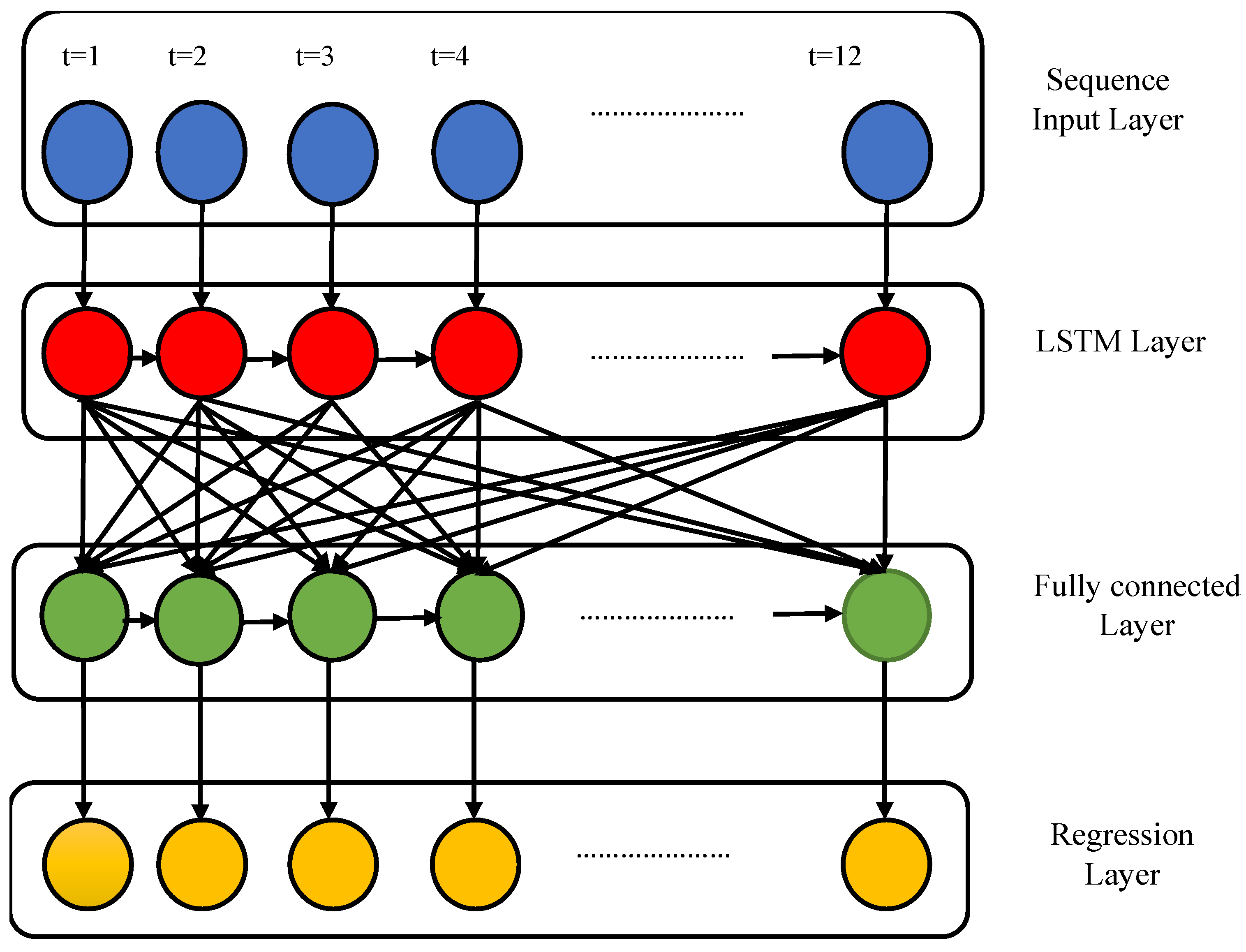
2.6. Deep Learning Network (RNN-LSTM)

ANN lacks a correlation approach and performs direct mapping between input and output data. The application of ANN in time series forecasting is therefore limited. To overcome this drawback, RNN builds up sequence to sequence mapping by adding up cyclic connections to neurons. The input of the previous time step affects the output of the next time step [57,58].

The use of contextual information for mapping between input and output is a key element of the RNN. The RNN loses the most deleted input information. However, RNN face the issue of gradient vanishing, as with ANN. The parameters are optimized in a negative way when the BP phenomena updates them. The gradient disappears, and the network is not updated. The performance of the classic RNN model is enhanced by using long short-term memory (LSTM) [59]. The RNN-LSTM is proposed to overcome the issues faced by regression, ANN, ANFIS and machine learning techniques. The RNN-layered LSTM’s structure is depicted in Figure 3. The sequence input layer, LSTM layer, fully connected layer, and regression output layer are the four layers that make up the proposed model. The four inputs, with one-hour resolution, are induced in the sequence input layer, with each input shown by a sole circle for 12 h a day. Layer 2 is an LSTM layer that works in flow with a fully linked layer to improve model performance. The LSTM layer analyzes numerous hidden units, whereas the fully connected layer displays a number of replies. Finally, the output is recorded by the regression layer.

The hyperparameters are optimally adjusted to improve the proposed model’s accuracy. The considered hyperparameters and their ranges are described in

Table 1. Range of the hyperparameters used in proposed model.

Hyperparameters	Range
The total number of hidden units	80–250
Maximum number of epochs	100–400
Initial rate of learning	50–200
Learn rate drop period	0.0001–0.01
Learn rate drop factor	0.002–1

. Different combinations of these hyperparameter values within the specified range are incorporated for simulation to evaluate the accuracy of the proposed model. Moreover, the constraints of the hyperparameters (epochs, hidden units) are defined because the response remains almost the same beyond the maximum value. It causes only wastage of time and resources. The optimal combination with lowest RMSE is chosen for better performance. Different LSTM structures are also investigated for each PV plant based on 2019 data to choose the best structure and to verify the concreteness of the proposed structure. The computing power for all simulation is Intel(R) Core (TM) i7-7500U CPU @ 2.70 GHz 2.90 GHz along with 64-bit operating system.

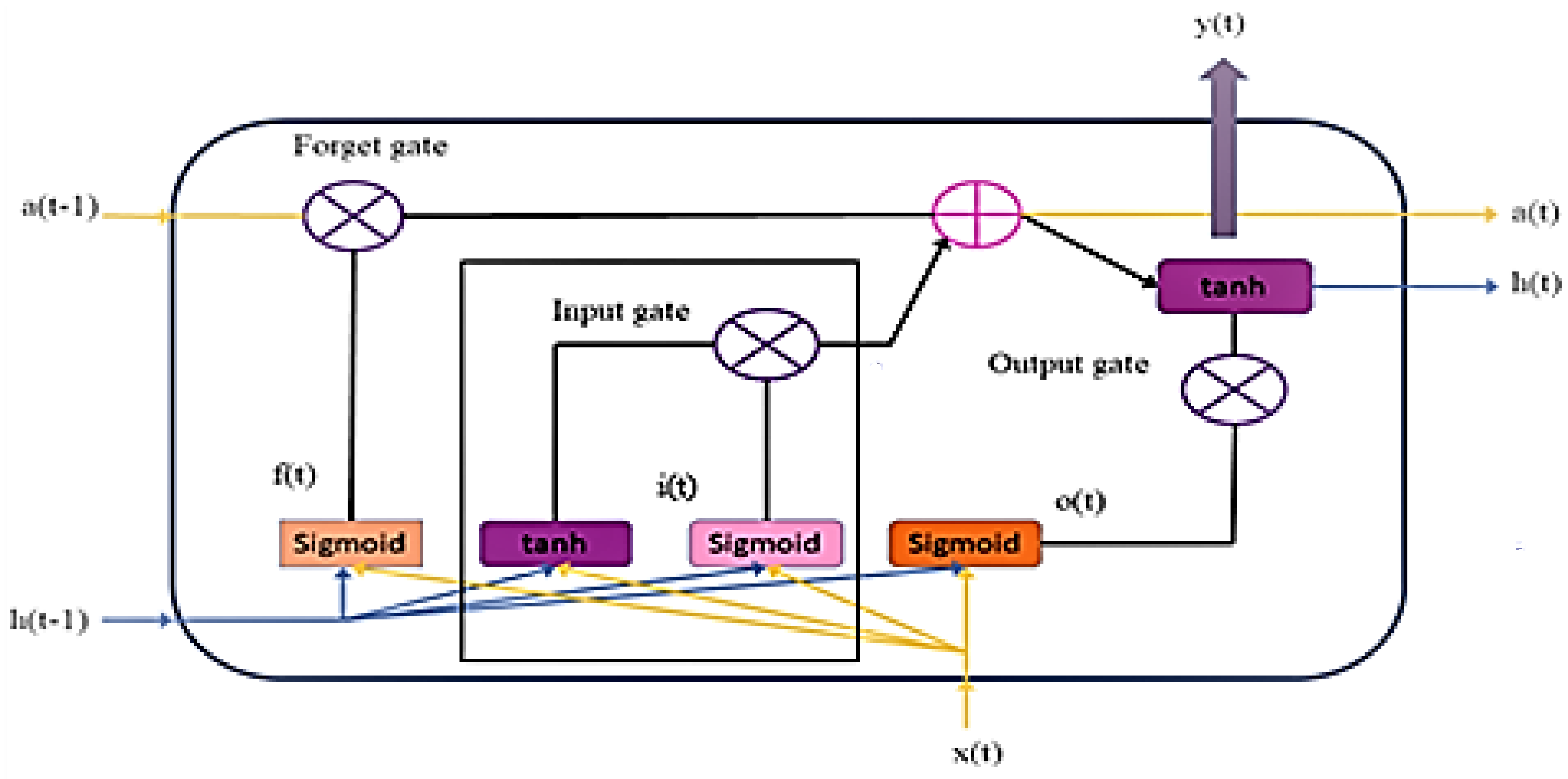
2.6.1. A Basic LSTM Structure

Figure 4 describes the basic LSTM cell structure. In RNN-LSTM, the subnets are referred to as memory units which consist of one or more than one memory cells. Furthermore, it consists of three types of gates known to be input, output and forget gates, all of which are impacted by x(t) and h(t − 1). Activation function, $\sigma$, often known as the sigmoid function, modulates the output coefficient value of these gates between 0 and 1 and is defined as follows [59]:

$$\sigma =\frac{1}{1+e^{-x}}$$

(11)

The LSTM cell’s basic operations are as follows:

• The LSTM cell decides whether the stored information from the previous cell state a(t − 1) should be removed. On activation, the forget gate receives the current and previous inputs and provides outputs in the form of zero and one. f(t) is calculated using the equation below [60].

  $$f\left(t\right)=\sigma \left[W_{xf}·X\left(t\right)+W_{hf}·h\left(t-1\right)+b_f\right]$$

  (12)
• The data to be stored in the cell is divided into two parts: $\overline{a\left(t\right)}$ and $i\left(t\right)$. The next state is decided by combining these two portions of information [60].

  $$tanh\left(x\right)=\frac{e^x-e^{-x}}{e^x+e^{-x}}$$

  (13)

  $$\overline{a\left(t\right)}=tanh\left(W_{xc}·X\left(t\right)+W_{hc}·h\left(t-1\right)+b_c\right)$$

  (14)

  $$i\left(t\right)=\mathsf{\sigma }\left(W_{xi}·X\left(t\right)+W_{hi}·h\left(t-1\right)+b_i\right)$$

  (15)
• The information from the previous stages is used to update the new cell state. By losing information in the first phase, f(t) is multiplied with the prior state a(t − 1). The generated information is multiplied by the input. Both components are added to decide the next state a(t), as shown in Equation (16) [60]:

  $$a\left(t\right)=f\left(t\right)·a\left(t-1\right)+i\left(t\right)·\overline{a\left(t\right)}$$

  (16)
• The final result is decoded in this stage. The hidden state h(t) is discovered by combining a(t)$·$tanh and o(t) in order to conserve important information. The output gate determines the output. The following are the equations for o(t), h(t), and y(t) [60]:

  $$o\left(t\right)=\sigma (W_{xo}·X(t)+W_{ho}·h(t-1)+b_o)$$

  (17)

  $$h\left(t\right)=o\left(t\right)·tanh\left[a\left(t\right)\right]$$

  (18)

  $$y\left(t\right)=\sigma (W_{hy}·h(t)+b_y)$$

  (19)

$W_{xf,}{W}_{xi,}{W}_{xo,}{W}_{xc}$ and $W_{hf,}{W}_{hi,}{W}_{ho,}{W}_{hc}$ are the input and recurrent weights matrices, while$W_{hy}$ is the weight bias for the hidden output. Corresponding bias vectors are $b_f,b_i,b_o,b_c$ and $b_y$. The forward and backward passes are used to train the LSTM neurons. The neuron weight is updated using the BPTT approach. The x(t) and y(t) are the input data and the PV power output, respectively, in this method.

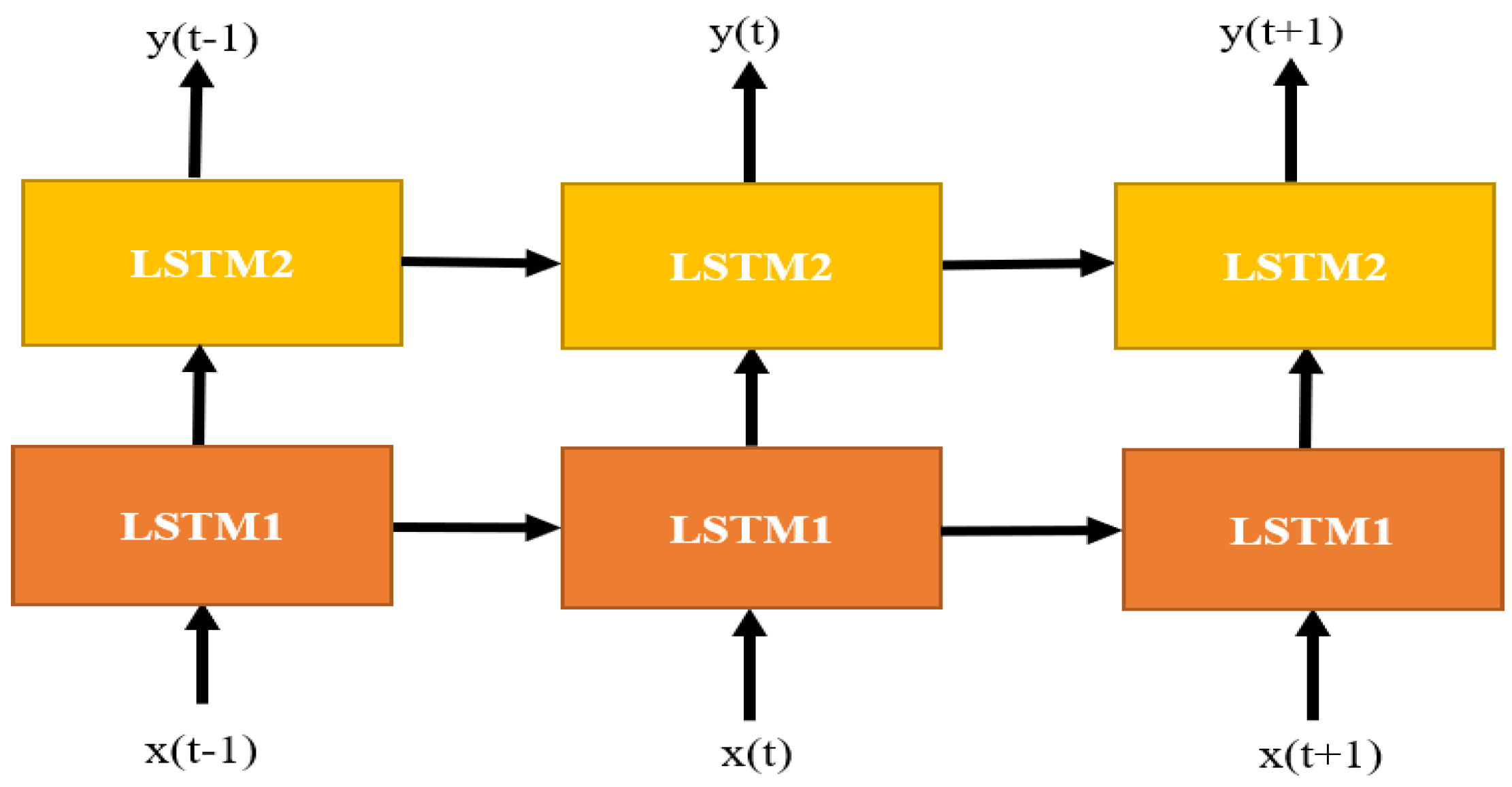
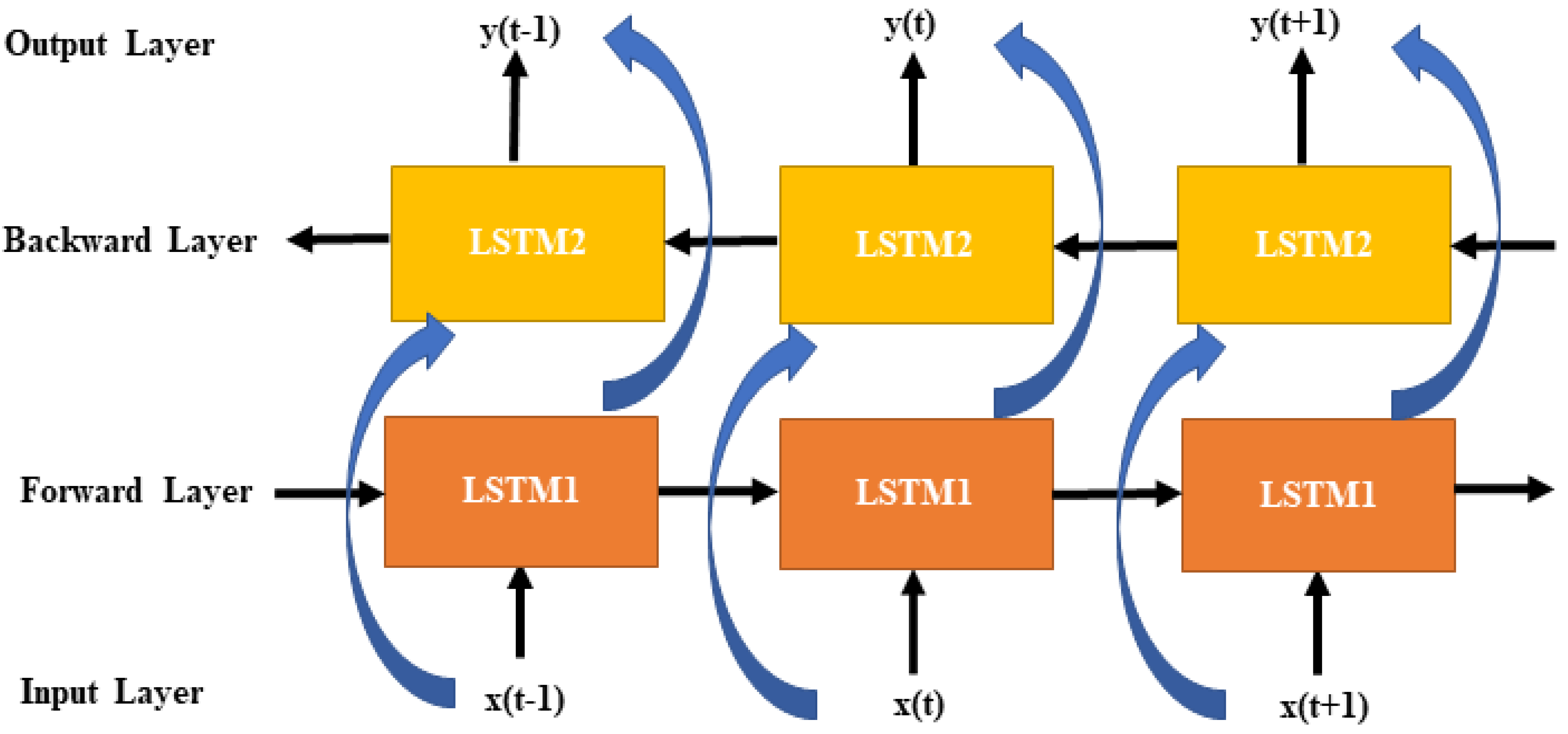
2.6.2. Multilayered LSTM Structures

In a basic LSTM, one hidden layer is used as in ANN. That hidden layer incorporates a certain number of hidden units. Following the theme of deep learning, more than one layer is added to enhance the prediction accuracy and training efficiency. Figure 5 further details the two-layered LSTM structure. The output of the preceding layer is used as the input of the succeeding layer at the specified time. In these multi-layered LSTM structures, information is only conveyed in one direction: forward.

Figure 6 describes a bi-directional LSTM, which represents both forward and backward transmission of information, connected with the output layer. The full previous and incoming information for each input pattern can be delivered to the output nodes using the bi-LSTM. The bi-LSTM has various applications in text recognition [61].

2.7. Performance Metrics to Measure Forecasting Accuracy

The following are the parameters that were used to evaluate the prediction model:

(a)

Root mean square error (RMSE):

$$\mathrm{RMSE}=\sqrt{\frac{1}{N}{\displaystyle \sum }_{i=1}^N{\left(X_i-Y_i\right)}^2}$$

(20)

(b)

Mean square error (MSE):

$$\mathrm{MSE}=\frac{1}{N}{\displaystyle \sum }_{i=1}^N{\left(X_i-Y_i\right)}^2$$

(21)

(c)

Mean absolute error (MAE):

$$\mathrm{MAE}=\frac{1}{N}{\displaystyle \sum }_{i=1}^N\left|\left(X_i-Y_i\right)\right|$$

(22)

(d)

Correlation coefficient (r):

$$r=\frac{{\sum }_{i=1}^N\left[\left(X_i-X_{avg}\right)\ast \left(Y_i-Y_{avg}\right)\right]}{\sqrt{{\sum }_{i=1}^N{\left(X_i-X_{avg}\right)}^2\ast {\sum }_{i=1}^N{\left(Y_i-Y_{avg}\right)}^2}}$$

(23)

(e)

Coefficient of determination (R²):

$$R^2=1-\frac{{\sum }_{i=1}^N{\left(X_i-Y_i\right)}^2}{{\sum }_{i=1}^N{\left(Y_i-Y_{avg}\right)}^2}$$

(24)

where $X_i$ and $Y_i$ represent the forecasted and real values, respectively, and the average values of these variables are represented by $X_{avg}$ and $Y_{avg}$. The RMSE is a measure of how far the anticipated value differs from the actual value. The MSE is used to calculate the mean square deviation between predicted and actual data. The mean absolute error, or MAE, is the absolute value of the average difference between predicted and actual values. The amount and direction of a linear relationship between two variables are indicated by the correlation coefficient (r). This varies between −1 and +1. A value of +1 represents strong correlation, while −1 shows a weak correlation. A value of r = 0 indicates no correlation between two variables. The coefficient of determination (R²) provides the percentage deviation in Y, which is explained by all the X variables together. The strength of the linear regression model is indicated by this number, which goes from 0 to 1. It is the same as the correlation coefficient squared. For the optimum performance model, r and R² have higher values and RMSE, MAE, and MSE have lower values.

3. Results and Discussions

3.1. LSTM Structure Comparison

Table 2. Comparison of different LSTM structures with RNN for power output prediction for three different PV plants using 2019 data.

LSTM Structures	p-si		m-si		a-si
	MAE	RMSE	MAE	RMSE	MAE	RSME
RNN-LSTM (single layered)	18.92	26.86	15.04	21.28	46.66	61.44
RNN-LSTM (double layered)	19.43	32.72	17.13	25.4	49.54	63.93
RNN-BiLSTM (single layered)	41.96	49	23.93	29.14	53.43	68.41

compares alternative LSTM architectures using 2019 data to demonstrate the superiority of the suggested technique (RNN-LSTM). It is clear from the table that single-layered LSTM performed better than the double-layered LSTM and single-layered bi-LSTM structures. The proposed RNN-LSTM technique (single-layered) showed the lowest testing MAE and RMSE for three PV plants when compared to other structures. This indicates that RNN-LSTM (single-layered) architecture is more feasible for implementation in forecasting the output PV power for all three PV plants (p-si, m-si and a-si).

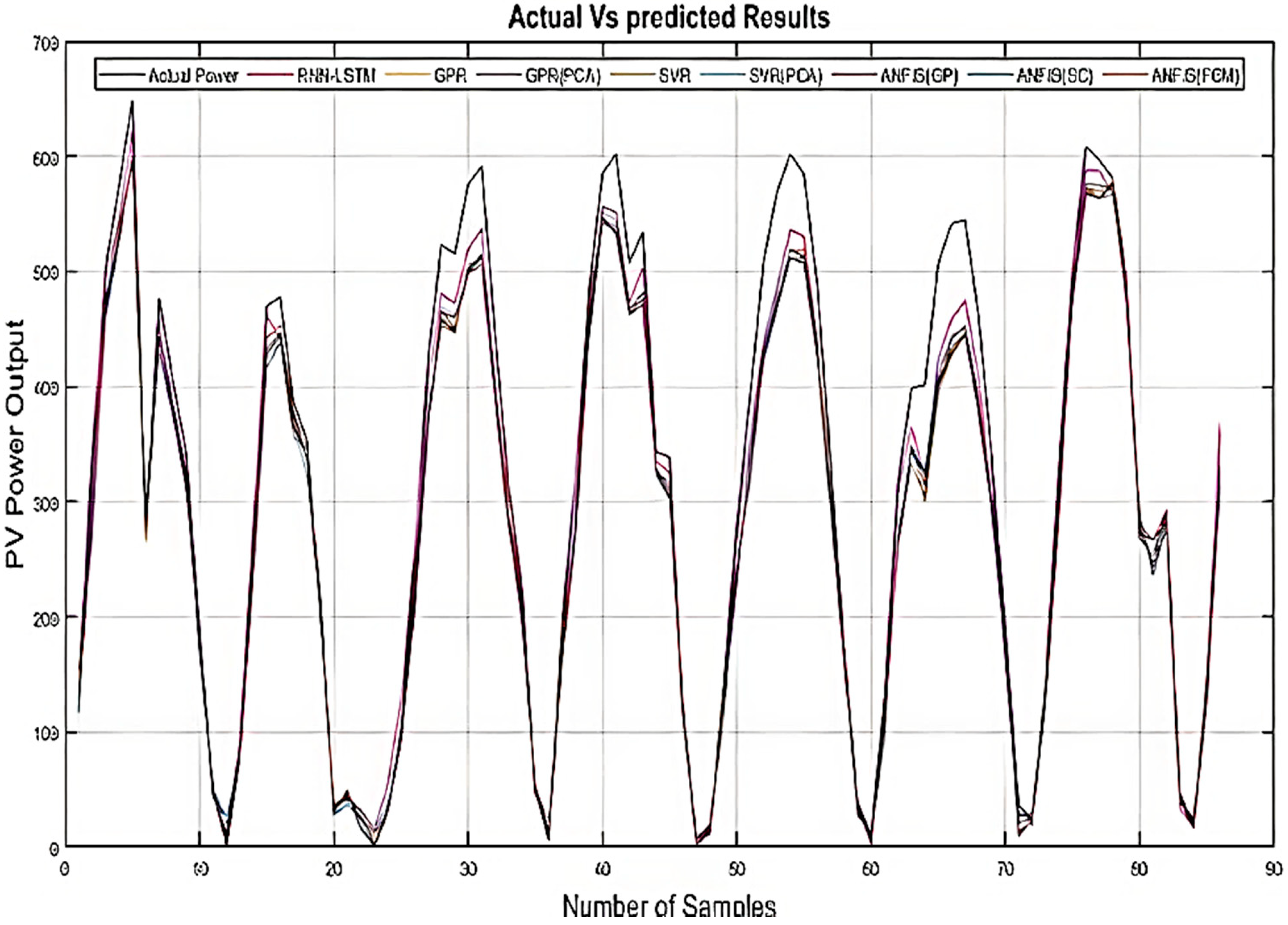
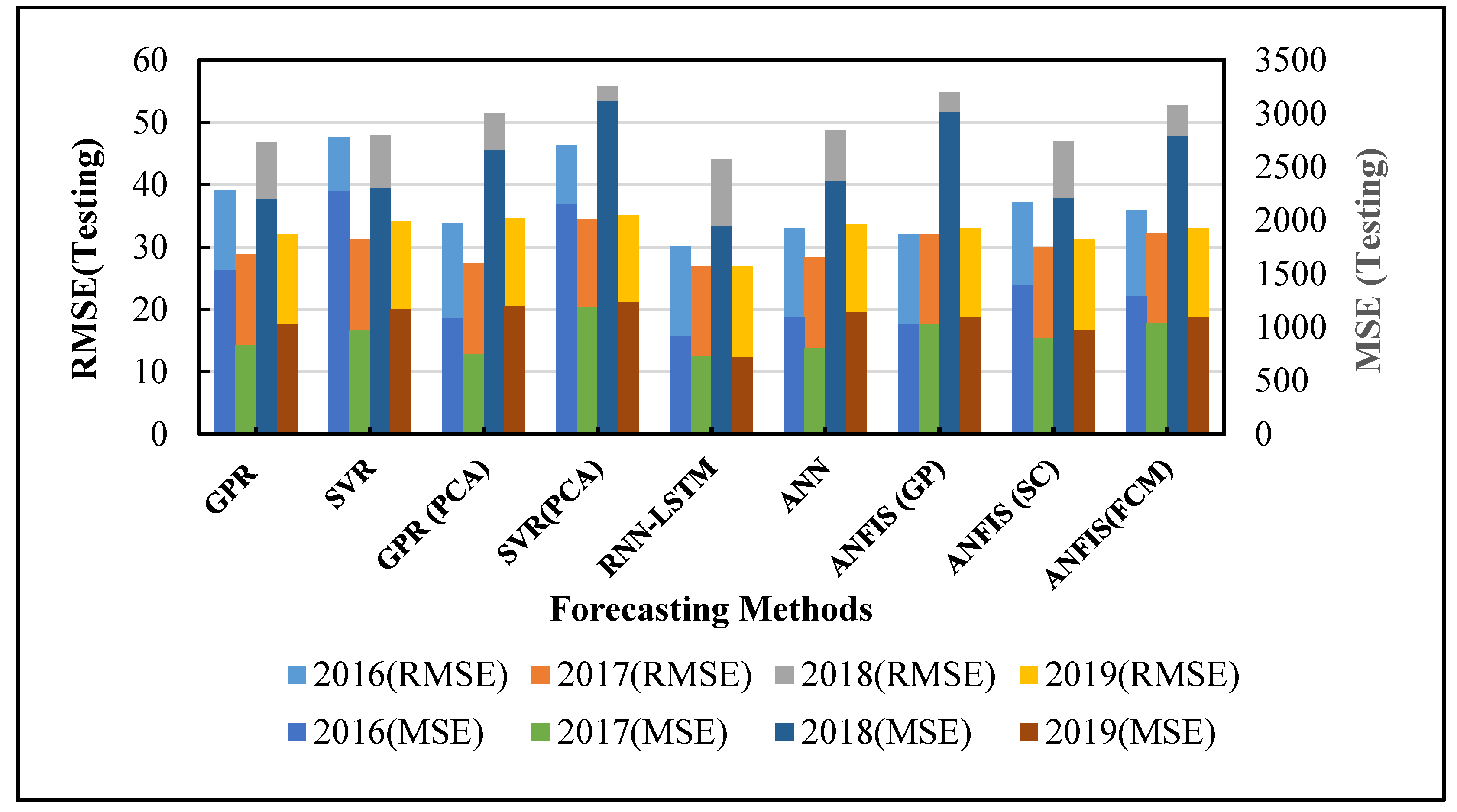
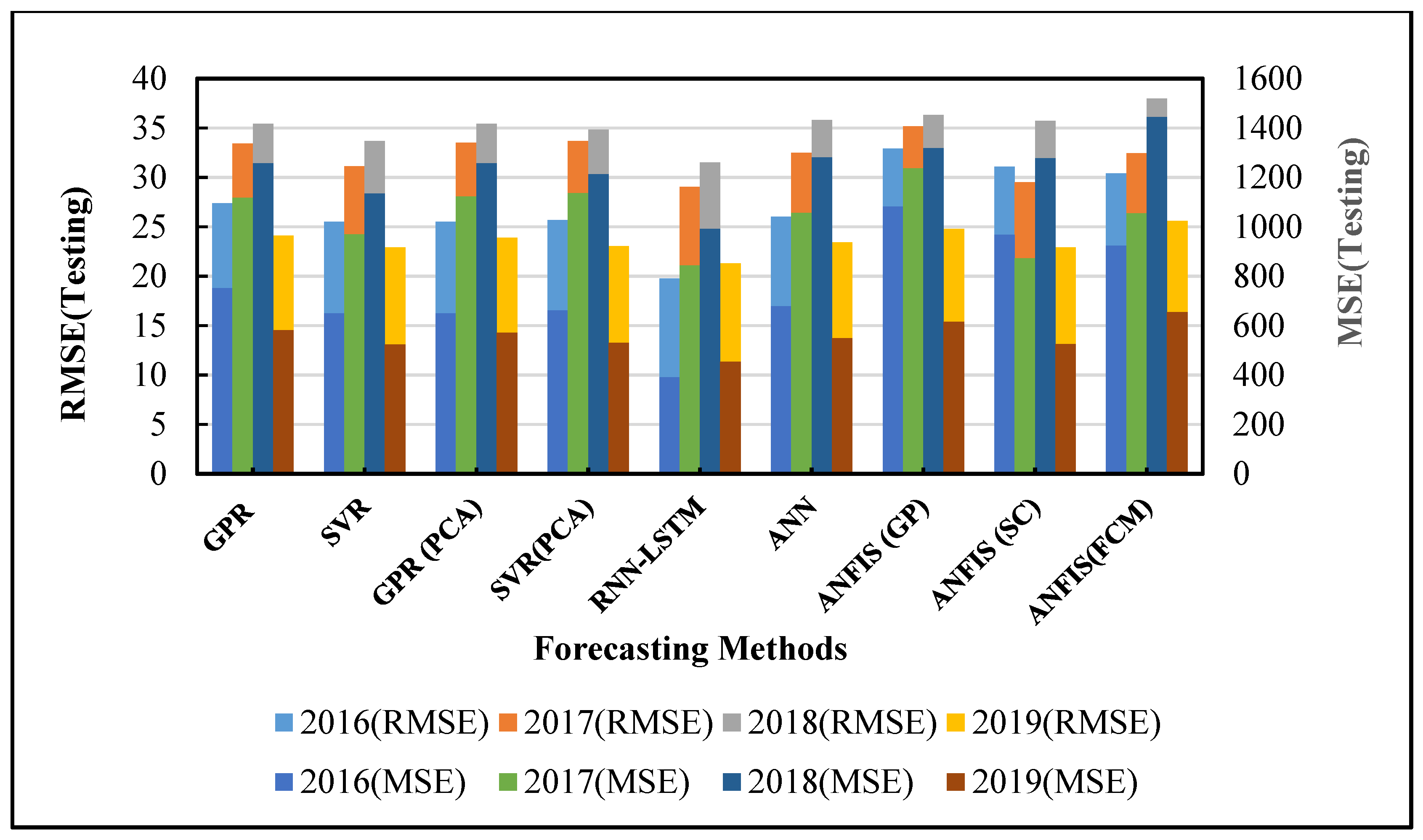
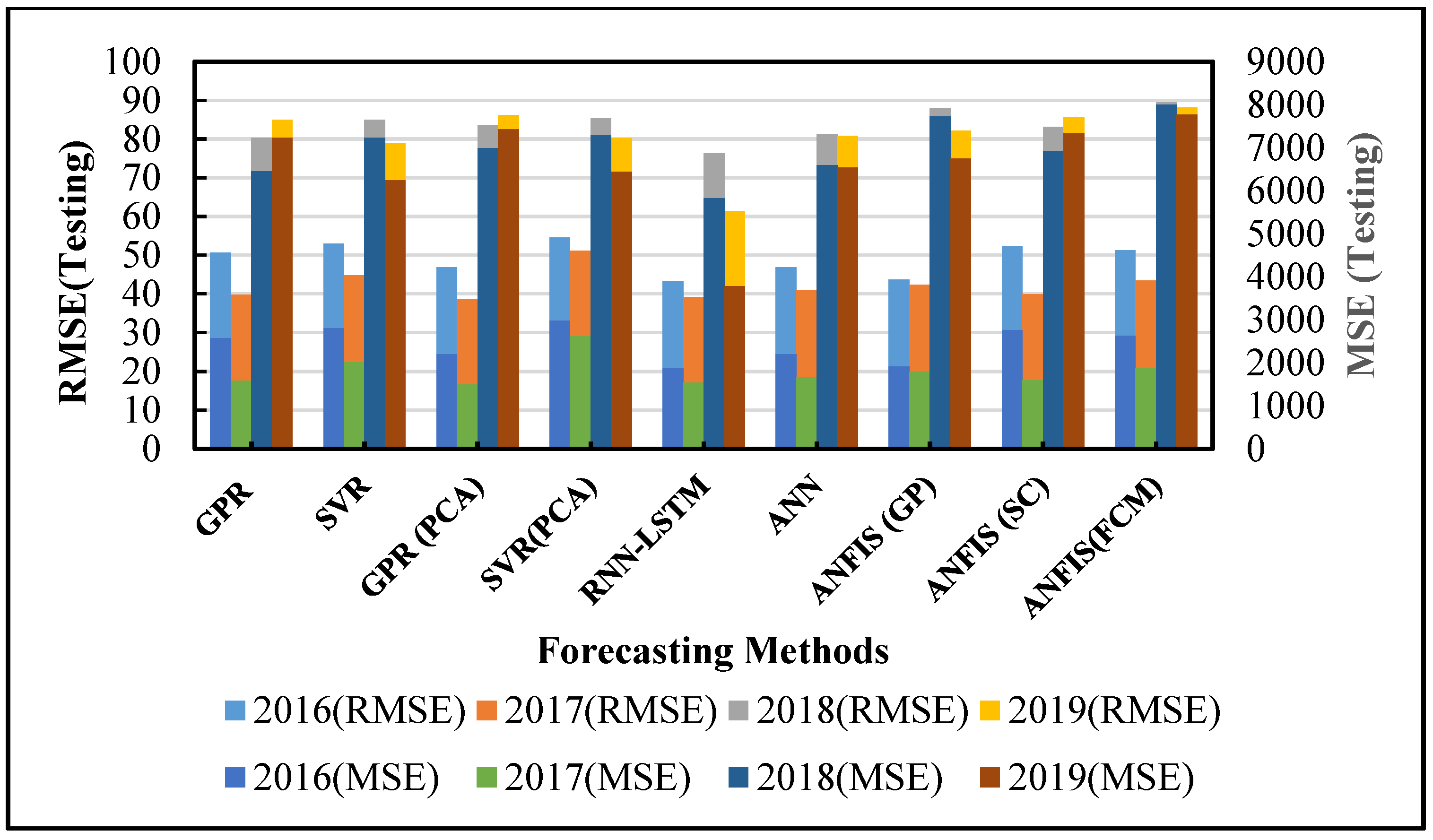
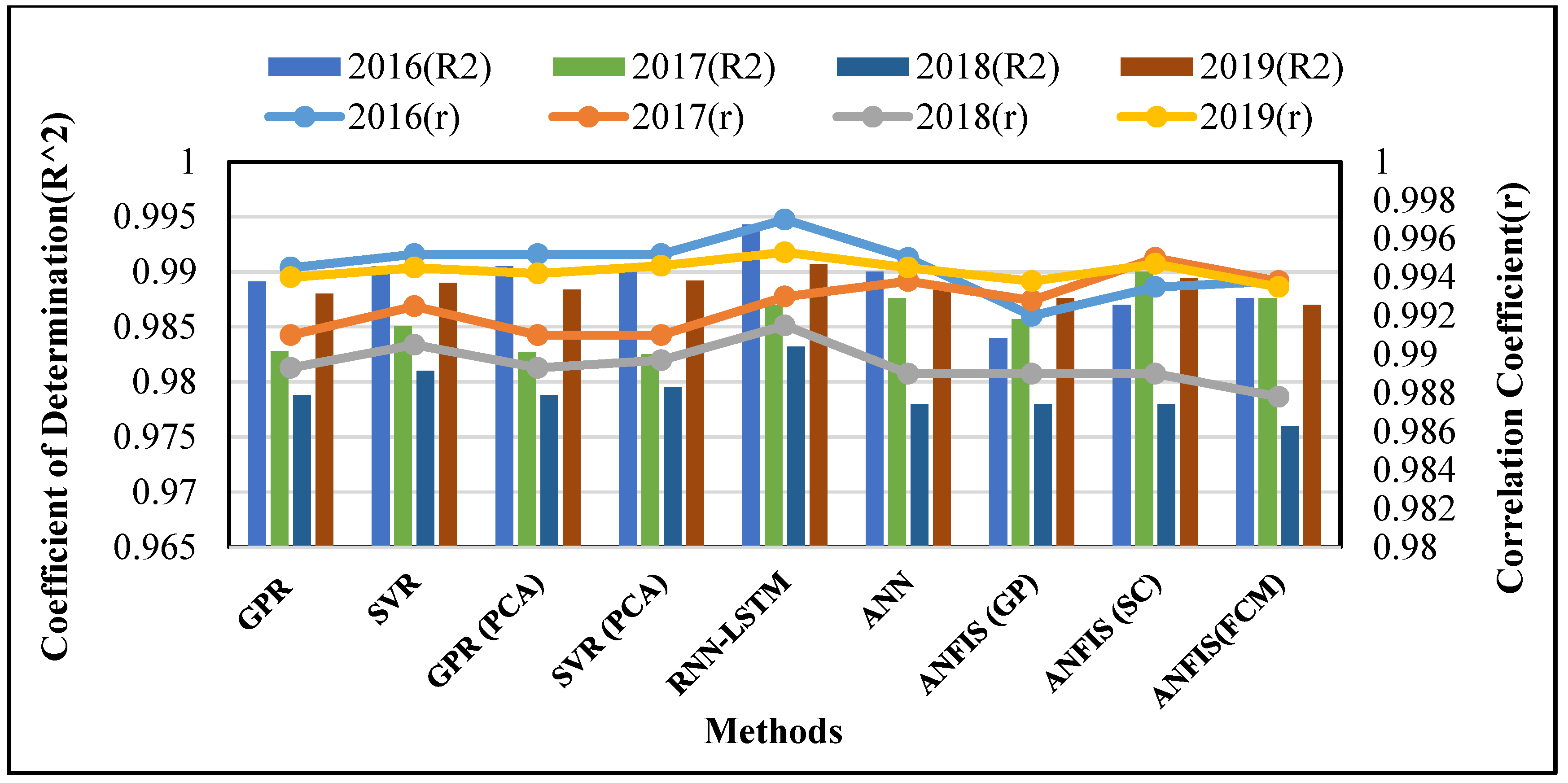
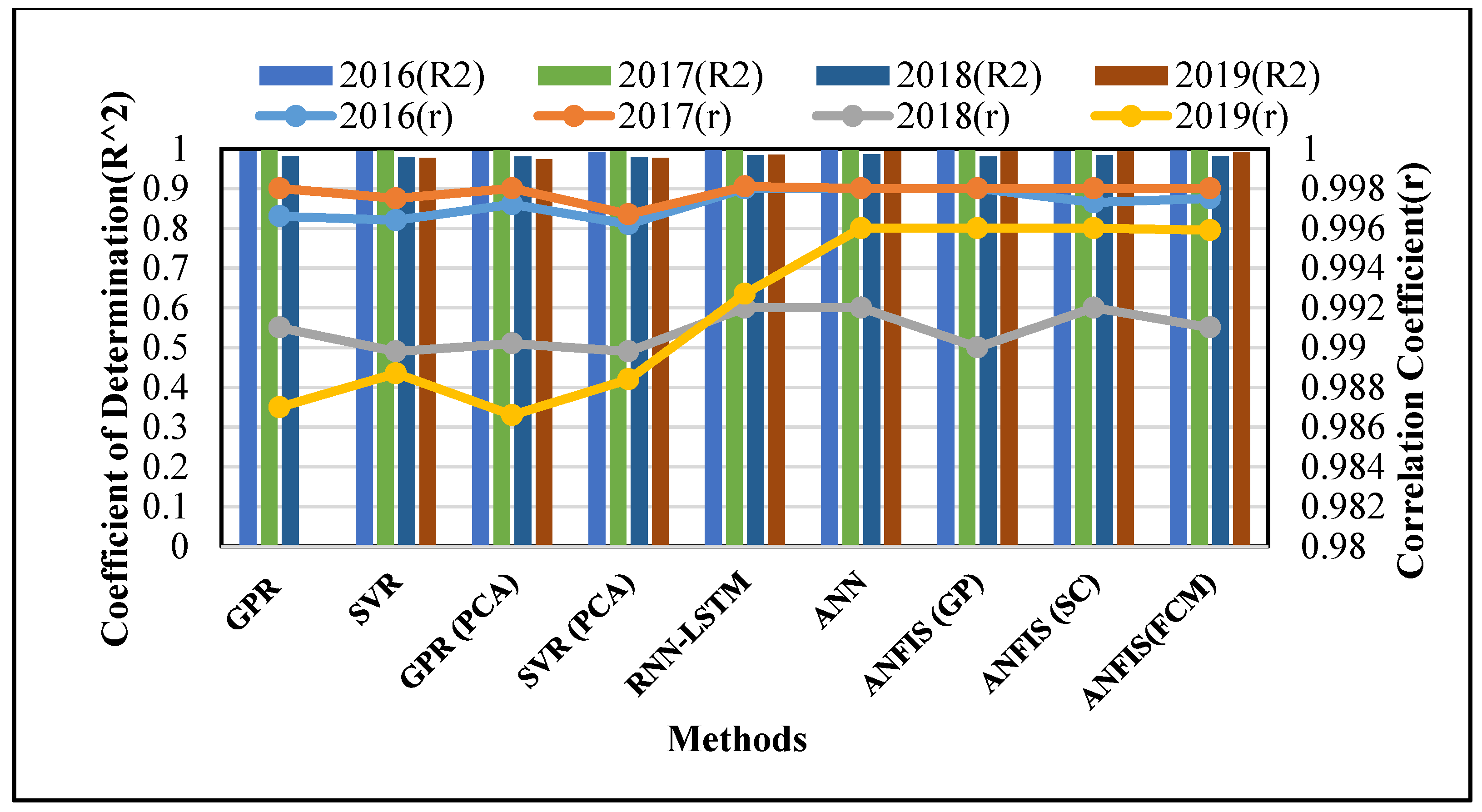
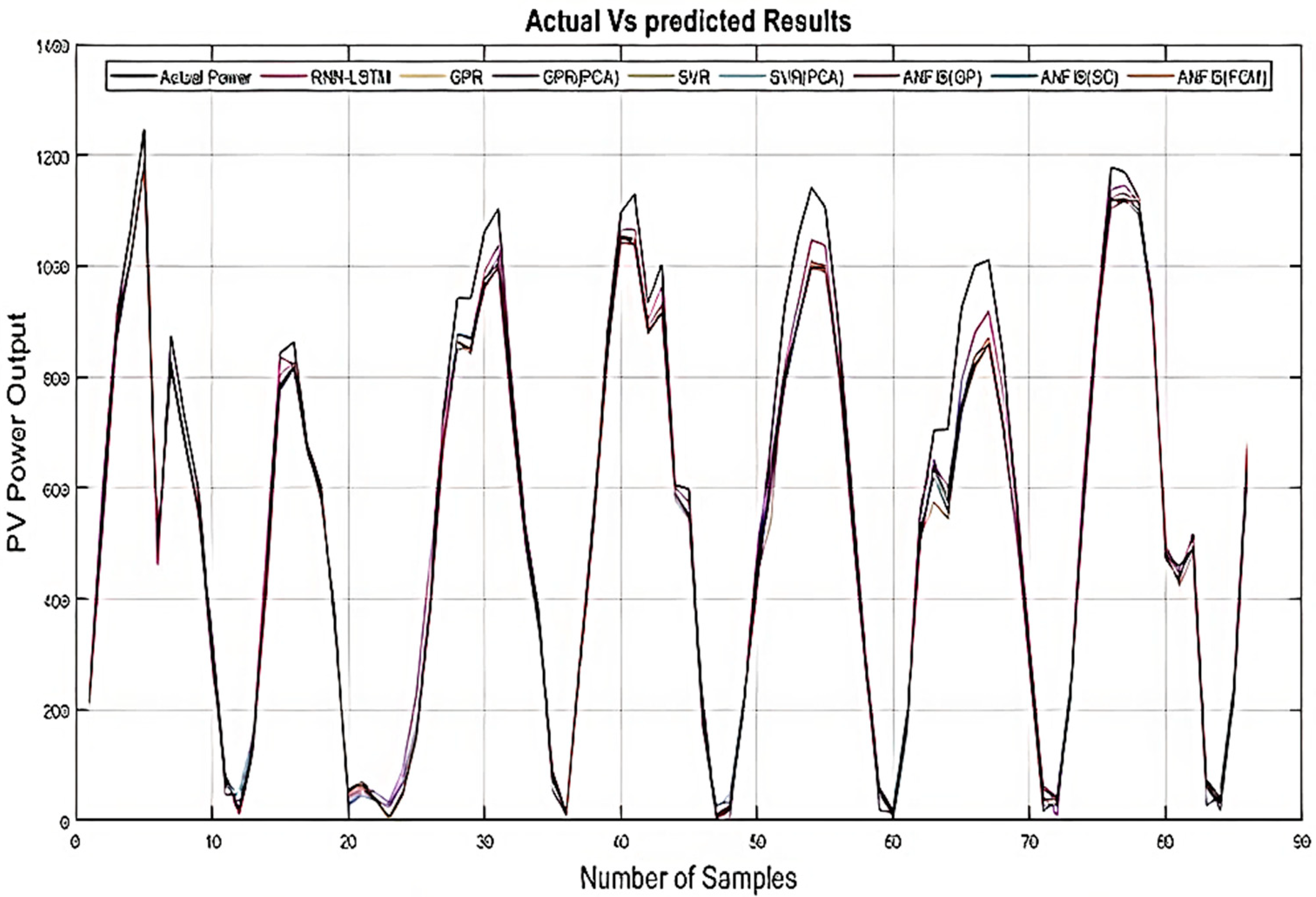
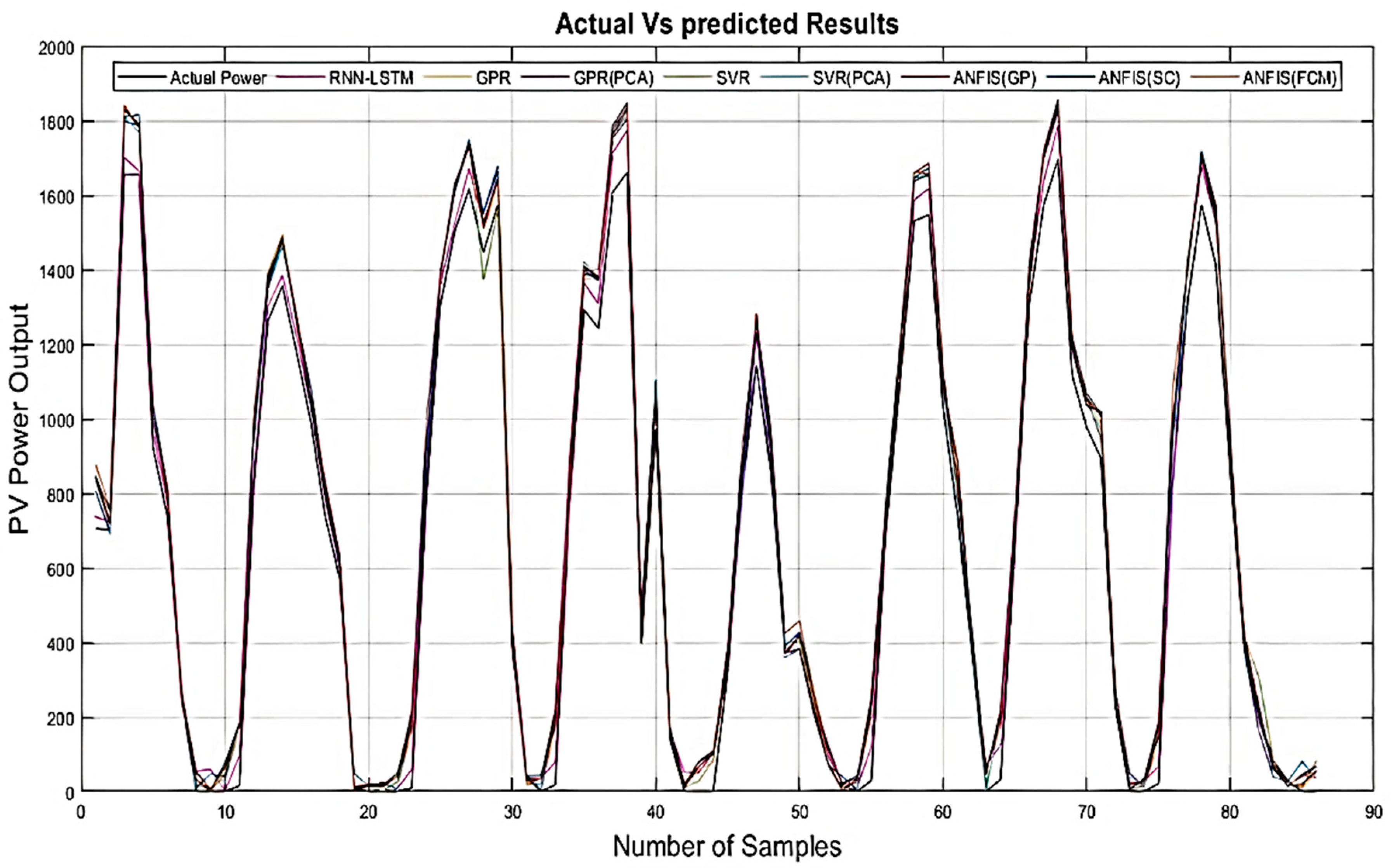
3.2. Forecasting Performance of Three PV Plants

This section discusses the performance findings of the suggested deep learning method, as well as of the linear and machine learning algorithms, for hour-ahead prediction of PV power output. The suggested technique (RNN-LSTM) was compared to other forecasting methods such as GPR, SVR, GPR(PCA), SVR(PCA), ANN, ANFIS(GP), ANFIS(SC) and ANFIS(FCM). The comparison was performed based on the same recorded data (2016–2019) on an annual basis for each of the three PV plants. For evaluation purposes, the data were subdivided into two parts: the training component, which consisted of 70% of input data, and the remaining 30% of the input data was for testing. The input parameters considered were the PV module and ambient temperatures, solar radiation, and wind speed, while the output parameter was the solar power output for each PV plant. The performance parameters used for system evaluation purposes were RMSE, MSE, MAE, r and R², as defined in Equations (20)–(24), respectively.

Based on the experimental results for the three PV plants over the four-year period from 2016 to 2019, the proposed RNN-LSTM exhibited the minimum training RMSE and MSE when compared with other techniques such as SVR, GPR, ANN, GPR(PCA), ANFIS(GP), SVR(PCA), ANFIS(FCM) and ANFIS(SC). Meanwhile, the training r and R² values of RNN-LSTM were also highest for all three PV plants in comparison with other applied techniques.

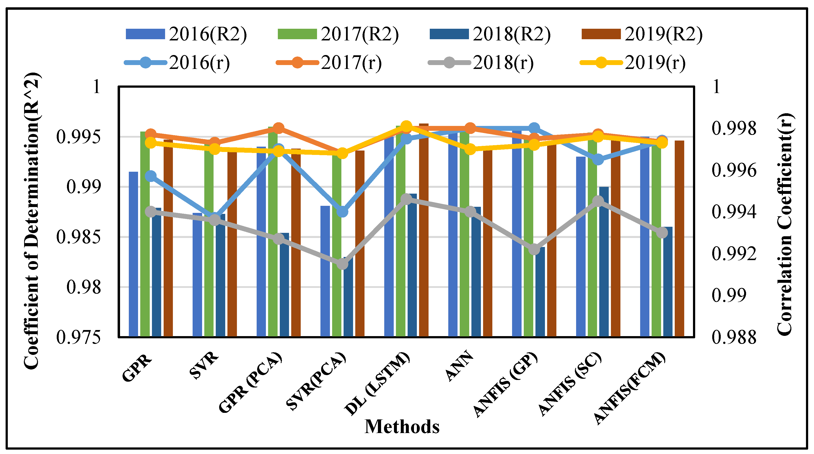
Statistical Analysis

Figure 7, Figure 8 and Figure 9 present the forecasting system’s yearly performance with respect to RMSE and MSE for all three (p-si, m-si, and a-si) PV plants for the timeframe of four years (2016–2019). In these three figures, RMSE and MSE are represented by solid and dotted lines. As shown in Figure 7, the suggested method resulted in test values of 30.25, 26.9, 44.06, 26.85, and 915.1, 723.52, 1941.2, 720.7, for RMSE and MSE, respectively, for p-si PV plants throughout the period of evaluation, which were the lowest compared to all other methods. The SVR (PCA) showed worst performance with the highest RMSE and MSE values in each year. For the m-si PV plant, as shown in Figure 8, the RNN-LSTM method gave lowest RMSE and MSE test values of 19.78, 29.04, 31.5, 21.28 and 391.1, 843.22, 991.9, 453.07, respectively, in contrast with all other methods over the period (2016–2019). The ANFIS (GP) presented the highest RMSE and MSE for 2016, 2017, and 2019, while for 2018, ANFIS (FCM) showed weak performance among all methods. The yearly statistics showed that testing RMSE of both p-si and m-si was lowest for the 2019 data and was highest for the 2018 data for all methods.

The suggested RNN-LSTM approach likewise showed the lowest test results of 43.37, 39.2, 76.31, 61.44 and 1881.3, 1536.64, 5822.5, 3774.87 of RMSE and MSE, respectively, over the duration (2016–2019) for a-si PV plants, as compared with all other methods shown in Figure 9. However, it exhibited comparative forecasting accuracy with GPR(PCA) for 2017. The SVR (PCA) presented weak performance for the 2016 and 2017 data, while ANFIS (FCM) was worst for the 2018 and 2019 data. All methods showed the highest RMSE for 2018 data in Figure 9. This may be due to missing data for some days because of power failure of the sensors. However, the missing data were reinstated using the data from a similar date in the previous or next year. The data for the remaining duration were properly synchronized and accurately retrieved without any synchronizing error.

Meanwhile, Figure 10, Figure 11 and Figure 12 show the computation of the determination coefficients (R²) and correlation coefficients (r) for the (p-si, m-si, and a-si) PV systems. Due to the close values, R² is represented by bar graphs on the primary axis, while r is shown by solid lines on the secondary axis. For all three PV plants, the suggested RNN-LSTM approach produced the greatest testing r and R² values for the time period (2016–2019). However, the r and R² values of the proposed method for a-si PV plants, based on 2019 data, were comparable with the ANN and ANFIS methods. Figure 10 shows that, for the p-si PV plant, the SVR and SVR (PCA) exhibited the lowest r values compared to all methods for (2016, 2017) and (2018, 2019) data, respectively. For the m-si system in Figure 11, the GPR and ANFIS (FCM) showed minimum values of r compared to all other methods for (2016, 2017) and (2018, 2019) data, respectively. The SVR (PCA) and ANFIS (FCM) showed minimum values of r compared to all other methods for the a-si PV plant, based on (2016, 2017 and 2018) and 2019 data, respectively, as shown in Figure 12.

Figure 13, Figure 14 and Figure 15 show the predicting outcomes for the developed deep learning approach (RNN-LSTM) and alternative forecasting models for three PV plants based only on 2019 data. When compared to previous approaches, the suggested method (RNN-LSTM) curve closely tracks the real power curve due to minimal variations in anticipated and real values. The reason is that when the RNN-LSTM technique is employed to estimate PV power output, the MSE and RMSE values are the lowest. The proposed model performed best for three distinct PV system materials and is thus practical and robust for forecasting PV power production for three different PV plants.

4. Summary

PV power output forecasting for one hour ahead was performed on yearly basis for three distinct types of PV plants during a four-year (2016–2019) timeframe. The proposed technique (RNN-LSTM) was compared with forecasting methods such as GPR, SVR, GPR(PCA), SVR(PCA), ANN, ANFIS(GP), ANFIS(SC), and ANFIS(FCM).

Forecasting accuracy was quantified using measures such as RMSE, MSE, MAE, r, and R². The suggested approach (RNN-LSTM) had the lowest (RMSE, MSE) and maximum (r, R²) testing values when compared to the other eight benchmark techniques for output PV power prediction at an hour ahead for all three PV plants on a yearly basis over the observed period (2016–2019). However, deep learning had comparable forecasting accuracy with GPR (PCA) for 2017 data and (ANN and ANFIS) for 2019 data, based on RMSE and (r, R²), respectively. Moreover, the comparison of different LSTM structures was also performed for 2019 data alone to show the dominance of the LSTM structure used in the proposed deep learning method (RNN-LSTM).

Furthermore, the p-si and a-si PV plants presented better prediction accuracy for 2017 than the other three years. For m-si plants, meanwhile, prediction accuracy for 2016 was better than for other years. On the other hand, all PV plants had the highest RMSE values for 2018 data, perhaps because some missing input data had been incorporated as a result of the power failure of recording sensors. The suggested technique also proved to be more reliable when it came to hourly power output forecasts for three distinct PV plants. In addition,

Table 3. Comparison of the suggested approach and benchmark methodologies in forecasting accuracy for different PV modules for the year 2016.

		Predicted Results			[38]
		RNN-LSTM	ANN	SVR	ELM	ANN	SVR
RMSE	p-si	30.25	33	47.63	54.96	60.27	71.92
	m-si	19.78	26.03	25.49	59.93	101.23	103.61
	a-si	43.37	46.9	52.92	90.41	101.99	145.38
R2	p-si	0.995	0.996	0.9874	0.9809	0.9798	0.9750
	m-si	0.9943	0.99	0.9905	0.8675	0.8647	0.8618
	a-si	0.996	0.996	0.9928	0.9783	0.9754	0.9704

compares the proposed method’s prediction accuracy to that of previous benchmark approaches [38] for similar site data in 2016. The RNN-LSTM and benchmark methods in this research showed better results than the given methods in [38].

Table 4. Comparison of the suggested method’s forecasting accuracy to the literature.

Methodology for Prediction	Ref	Year	Testing RMSE (W/m2)
RNN-LSTM (p-si)	Present study	-	26.85
RNN-LSTM (m-si)	Present study	-	19.78
RNN-LSTM (Thin film)	Present study	-	39.2
LSTM	[62]	2018	139.3
LSTM	[46]	2018	122.7
LSTM	[46]	2018	76.24
LSTM	[63]	2018	<29.26

compares the suggested method’s forecasting accuracy to the approaches addressed in the literature. This table shows the lowest testing RMSE for each PV plant over the last four years (2016–2019). When compared to the findings of prior studies, the proposed technique had the lowest testing RMSE for all three PV plants.

5. Conclusions

For hour-ahead prediction of output PV power, this study compared the predicting accuracy of the suggested deep learning method (RNN-LSTM) to regression (GPR, GPR (PCA)), machine learning (SVR, ANN, SVR (PCA)), and hybrid (ANFIS) methodologies for three different PV plants (p-si, m-si, and a-si). For four years of data (2016–2019), predictions were made on an annual basis. The MAE, MSE, RMSE, coefficient of correlation (r), and determination (R²) were used to evaluate the forecasting accuracy of the recommended and other applicable approaches.

In contrast to the existing methodologies, the suggested RNN-LSTM exhibited the lowest testing RMSE and MSE values for p-si and m-si PV plants during the four-year timeframe (2016–2019). Meanwhile, the suggested technique had the lowest testing RMSE of (43.37, 39.2, 76.31 and 61.44), over the years 2016, 2017, 2018 and 2019, respectively, for thin-film PV plants. Furthermore, when compared to previous approaches, the suggested method demonstrated improved r and R² values for all three PV plants for practically all of the years. The findings also indicated that, based on 2019 data alone, the single-layered LSTM had greater predicting accuracy in terms of reduced MAE and RMSE than other LSTM structures, proving the superiority of the suggested strategy (RNN-LSTM).

It can be concluded that the suggested RNN-LSTM has demonstrated superior forecasting accuracy for solar power output forecasting at an hour ahead on an annual basis over a four-year timeframe when compared to other approaches, such as to regression (GPR (PCA), GPR), machine learning (ANN, SVR, SVR (PCA)) and hybrid (ANFIS) methods. Moreover, the proposed method was found to be robust, showing better forecasting accuracy for three different PV plants. Further study can be performed in the future by incorporating some optimization algorithms with RNN-LSTM to optimize hyperparameters and enhance its prediction accuracy.

References

1. Shafiee, S.; Topal, E. When will fossil fuel reserves be diminished? Energy Policy 2009, 37, 181–189. [Google Scholar] [CrossRef]
2. Wang, F.; Xuan, Z.; Zhen, Z.; Li, K.; Wang, T.; Shi, M. A day-ahead PV power forecasting method based on LSTM-RNN model and time correlation modification under partial daily pattern prediction framework. Energy Convers. Manag. 2020, 212, 112766. [Google Scholar] [CrossRef]
3. Khanlari, A.; Sözen, A.; Şirin, C.; Tuncer, A.D.; Gungor, A. Performance enhancement of a greenhouse dryer: Analysis of a cost-effective alternative solar air heater. J. Clean. Prod. 2020, 251, 119672. [Google Scholar] [CrossRef]
4. Ağbulut, Ü.; Gürel, A.E.; Ergün, A.; Ceylan, İ. Performance assessment of a V-trough photovoltaic system and prediction of power output with different machine learning algorithms. J. Clean. Prod. 2020, 268, 122269. [Google Scholar] [CrossRef]
5. Das, U.K.; Tey, K.S.; Seyedmahmoudian, M.; Mekhilef, S.; Idris, M.Y.I.; Van Deventer, W.; Horan, B.; Stojcevski, A. Forecasting of photovoltaic power generation and model optimization: A review. Renew. Sustain. Energy Rev. 2018, 81, 912–928. [Google Scholar] [CrossRef]
6. Mellit, A.; Kalogirou, S.A.; Hontoria, L.; Shaari, S. Artificial intelligence techniques for sizing photovoltaic systems: A review. Renew. Sustain. Energy Rev. 2009, 13, 406–419. [Google Scholar] [CrossRef]
7. Memon, M.A.; Mekhilef, S.; Mubin, M.; Aamir, M. Selective harmonic elimination in inverters using bio-inspired intelligent algorithms for renewable energy conversion applications: A review. Renew. Sustain. Energy Rev. 2017, 82 Pt 3, 2235–2253. [Google Scholar] [CrossRef]
8. Xin-gang, Z.; You, Z. Technological progress and industrial performance: A case study of solar photovoltaic industry. Renew. Sustain. Energy Rev. 2018, 81, 929–936. [Google Scholar] [CrossRef]
9. Wang, F.; Xu, H.; Xu, T.; Li, K.; Shafie-khah, M.; Catalão, J.P.S. The values of market-based demand response on improving power system reliability under extreme circumstances. Appl. Energy 2017, 193, 220–231. [Google Scholar] [CrossRef]
10. Li, K.; Wang, F.; Mi, Z.; Fotuhi-Firuzabad, M.; Duić, N.; Wang, T. Capacity and output power estimation approach of individual behind-the-meter distributed photovoltaic system for demand response baseline estimation. Appl. Energy 2019, 253, 113595. [Google Scholar] [CrossRef]
11. Wang, F.; Ge, X.; Li, K.; Mi, Z. Day-Ahead Market Optimal Bidding Strategy and Quantitative Compensation Mechanism Design for Load Aggregator Engaging Demand Response. IEEE Trans. Ind. Appl. 2019, 55, 5564–5573. [Google Scholar] [CrossRef]
12. Reikard, G.; Hansen, C. Forecasting solar irradiance at short horizons: Frequency and time domain models. Renew. Energy 2019, 135, 1270–1290. [Google Scholar] [CrossRef]
13. Wang, J.; Li, Q.; Zeng, B. Multi-layer cooperative combined forecasting system for short-term wind speed forecasting. Sustain. Energy Technol. Assess. 2021, 43, 100946. [Google Scholar] [CrossRef]
14. Akhter, M.N.; Mekhilef, S.; Mokhlis, H.; Shah, N.M. Review on forecasting of photovoltaic power generation based on machine learning and metaheuristic techniques. IET Renew. Power Gener. 2019, 13, 1009–1023. [Google Scholar] [CrossRef] [Green Version]
15. Pierro, M.; Bucci, F.; De Felice, M.; Maggioni, E.; Perotto, A.; Spada, F.; Moser, D.; Cornaro, C. Deterministic and stochastic approaches for day-ahead solar power forecasting. J. Sol. Energy Eng. 2017, 139, 021010. [Google Scholar] [CrossRef]
16. Prema, V.; Rao, K.U. Development of statistical time series models for solar power prediction. Renew. Energy 2015, 83, 100–109. [Google Scholar] [CrossRef]
17. Hirata, Y.; Aihara, K. Improving time series prediction of solar irradiance after sunrise: Comparison among three methods for time series prediction. Sol. Energy 2017, 149, 294–301. [Google Scholar] [CrossRef]
18. Shireen, T.; Shao, C.; Wang, H.; Li, J.; Zhang, X.; Li, M. Iterative multi-task learning for time-series modeling of solar panel PV outputs. Appl. Energy 2018, 212, 654–662. [Google Scholar] [CrossRef]
19. Bigdeli, N.; Salehi Borujeni, M.; Afshar, K. Time series analysis and short-term forecasting of solar irradiation, a new hybrid approach. Swarm Evol. Comput. 2017, 34, 75–88. [Google Scholar] [CrossRef]
20. Wang, F.; Zhen, Z.; Liu, C.; Mi, Z.; Hodge, B.-M.; Shafie-khah, M.; Catalão, J.P.S. Image phase shift invariance based cloud motion displacement vector calculation method for ultra-short-term solar PV power forecasting. Energy Convers. Manag. 2018, 157, 123–135. [Google Scholar] [CrossRef]
21. Zaher, A.; Thil, S.; Nou, J.; Traoré, A.; Grieu, S. Comparative study of algorithms for cloud motion estimation using sky-imaging data. IFAC-PapersOnLine 2017, 50, 5934–5939. [Google Scholar] [CrossRef]
22. Cheng, H.-Y. Cloud tracking using clusters of feature points for accurate solar irradiance nowcasting. Renew. Energy 2017, 104, 281–289. [Google Scholar] [CrossRef]
23. Lima, F.J.L.; Martins, F.R.; Pereira, E.B.; Lorenz, E.; Heinemann, D. Forecast for surface solar irradiance at the Brazilian Northeastern region using NWP model and artificial neural networks. Renew. Energy 2016, 87, 807–818. [Google Scholar] [CrossRef]
24. Perez, R.; Lorenz, E.; Pelland, S.; Beauharnois, M.; Van Knowe, G.; Hemker, K.; Heinemann, D.; Remund, J.; Müller, S.C.; Traunmüller, W.; et al. Comparison of numerical weather prediction solar irradiance forecasts in the US, Canada and Europe. Sol. Energy 2013, 94, 305–326. [Google Scholar] [CrossRef]
25. Verzijlbergh, R.A.; Heijnen, P.W.; de Roode, S.R.; Los, A.; Jonker, H.J.J. Improved model output statistics of numerical weather prediction based irradiance forecasts for solar power applications. Sol. Energy 2015, 118, 634–645. [Google Scholar] [CrossRef]
26. Mathiesen, P.; Collier, C.; Kleissl, J. A high-resolution, cloud-assimilating numerical weather prediction model for solar irradiance forecasting. Sol. Energy 2013, 92, 47–61. [Google Scholar] [CrossRef] [Green Version]
27. Hussain, S.; AlAlili, A. A hybrid solar radiation modeling approach using wavelet multiresolution analysis and artificial neural networks. Appl. Energy 2017, 208, 540–550. [Google Scholar] [CrossRef]
28. Xue, X. Prediction of daily diffuse solar radiation using artificial neural networks. Int. J. Hydrog. Energy 2017, 42, 28214–28221. [Google Scholar] [CrossRef]
29. Alzahrani, A.; Shamsi, P.; Dagli, C.; Ferdowsi, M. Solar Irradiance Forecasting Using Deep Neural Networks. Procedia Comput. Sci. 2017, 114, 304–313. [Google Scholar] [CrossRef]
30. Bou-Rabee, M.; Sulaiman, S.A.; Saleh, M.S.; Marafi, S. Using artificial neural networks to estimate solar radiation in Kuwait. Renew. Sustain. Energy Rev. 2017, 72, 434–438. [Google Scholar] [CrossRef]
31. Olatomiwa, L.; Mekhilef, S.; Shamshirband, S.; Petković, D.J.R.; Reviews, S.E. Adaptive neuro-fuzzy approach for solar radiation prediction in Nigeria. Renew. Sustain. Energy Rev. 2015, 51, 1784–1791. [Google Scholar] [CrossRef]
32. Dolara, A.; Grimaccia, F.; Leva, S.; Mussetta, M.; Ogliari, E. A physical hybrid artificial neural network for short term forecasting of PV plant power output. Energies 2015, 8, 1138–1153. [Google Scholar] [CrossRef] [Green Version]
33. De Giorgi, M.; Malvoni, M.; Congedo, P. Comparison of strategies for multi-step ahead photovoltaic power forecasting models based on hybrid group method of data handling networks and least square support vector machine. Energy 2016, 107, 360–373. [Google Scholar] [CrossRef]
34. Jang, H.S.; Bae, K.Y.; Park, H.-S.; Sung, D.K. Solar power prediction based on satellite images and support vector machine. IEEE Trans. Sustain. Energy 2016, 7, 1255–1263. [Google Scholar] [CrossRef]
35. Da Silva Fonseca, J.G., Jr.; Oozeki, T.; Ohtake, H.; Shimose, K.-i.; Takashima, T.; Ogimoto, K. Forecasting regional photovoltaic power generation-a comparison of strategies to obtain one-day-ahead data. Energy Procedia 2014, 57, 1337–1345. [Google Scholar]
36. Wolff, B.; Kühnert, J.; Lorenz, E.; Kramer, O.; Heinemann, D. Comparing support vector regression for PV power forecasting to a physical modeling approach using measurement, numerical weather prediction, and cloud motion data. Sol. Energy 2016, 135, 197–208. [Google Scholar] [CrossRef]
37. Tang, P.; Chen, D.; Hou, Y. Entropy method combined with extreme learning machine method for the short-term photovoltaic power generation forecasting. Chaos Solitons Fractals 2016, 89, 243–248. [Google Scholar] [CrossRef]
38. Hossain, M.; Mekhilef, S.; Danesh, M.; Olatomiwa, L.; Shamshirband, S. Application of extreme learning machine for short term output power forecasting of three grid-connected PV systems. J. Clean. Prod. 2017, 167, 395–405. [Google Scholar] [CrossRef]
39. Deo, R.C.; Downs, N.; Parisi, A.V.; Adamowski, J.F.; Quilty, J.M. Very short-term reactive forecasting of the solar ultraviolet index using an extreme learning machine integrated with the solar zenith angle. Environ. Res. 2017, 155, 141–166. [Google Scholar] [CrossRef] [PubMed]
40. Youssef, A.; El-Telbany, M.; Zekry, A. The role of artificial intelligence in photo-voltaic systems design and control: A review. Renew. Sustain. Energy Rev. 2017, 78, 72–79. [Google Scholar] [CrossRef]
41. Wang, H.; Lei, Z.; Zhang, X.; Zhou, B.; Peng, J. A review of deep learning for renewable energy forecasting. Energy Convers. Manag. 2019, 198, 111799. [Google Scholar] [CrossRef]
42. Narvaez, G.; Giraldo, L.F.; Bressan, M.; Pantoja, A. Machine learning for site-adaptation and solar radiation forecasting. Renew. Energy 2021, 167, 333–342. [Google Scholar] [CrossRef]
43. Wang, K.; Qi, X.; Liu, H. A comparison of day-ahead photovoltaic power forecasting models based on deep learning neural network. Appl. Energy 2019, 251, 113315. [Google Scholar] [CrossRef]
44. Luo, X.; Zhang, D.; Zhu, X. Deep learning based forecasting of photovoltaic power generation by incorporating domain knowledge. Energy 2021, 225, 120240. [Google Scholar] [CrossRef]
45. Chang, G.W.; Lu, H.-J. Integrating Gray Data Preprocessor and Deep Belief Network for Day-Ahead PV Power Output Forecast. IEEE Trans. Sustain. Energy 2018, 11, 185–194. [Google Scholar] [CrossRef]
46. Qing, X.; Niu, Y.J.E. Hourly day-ahead solar irradiance prediction using weather forecasts by LSTM. Energy 2018, 148, 461–468. [Google Scholar] [CrossRef]
47. Nour-eddine, I.O.; Lahcen, B.; Fahd, O.H.; Amin, B.; Aziz, O. Power forecasting of three silicon-based PV technologies using actual field measurements. Sustain. Energy Technol. Assess. 2021, 43, 100915. [Google Scholar] [CrossRef]
48. Halabi, L.M.; Mekhilef, S.; Hossain, M. Performance evaluation of hybrid adaptive neuro-fuzzy inference system models for predicting monthly global solar radiation. Appl. Energy 2018, 213, 247–261. [Google Scholar] [CrossRef]
49. Akhter, M.N.; Mekhilef, S.; Mokhlis, H.; Olatomiwa, L.; Muhammad, A. Performance assessment of three grid-connected photovoltaic systems with combined capacity of 6.575 kWp in Malaysia. J. Clean. Prod. 2020, 277, 123242. [Google Scholar] [CrossRef]
50. Najibi, F.; Apostolopoulou, D.; Alonso, E. Enhanced performance Gaussian process regression for probabilistic short-term solar output forecast. Int. J. Electr. Power Energy Syst. 2021, 130, 106916. [Google Scholar] [CrossRef]
51. Quej, V.H.; Almorox, J.; Arnaldo, J.A.; Saito, L. ANFIS, SVM and ANN soft-computing techniques to estimate daily global solar radiation in a warm sub-humid environment. J. Atmos. Sol.-Terr. Phys. 2017, 155, 62–70. [Google Scholar] [CrossRef] [Green Version]
52. Lotfi, H.; Adar, M.; Bennouna, A.; Izbaim, D.; Oum’bark, F.; Ouacha, H. Silicon Photovoltaic Systems Performance Assessment Using the Principal Component Analysis Technique. Mater. Today Proc. 2021, 51, 966–1974. [Google Scholar] [CrossRef]
53. Adar, M.; Najih, Y.; Gouskir, M.; Chebak, A.; Mabrouki, M.; Bennouna, A. Three PV plants performance analysis using the principal component analysis method. Energy 2020, 207, 118315. [Google Scholar] [CrossRef]
54. Khosravi, A.; Koury, R.; Machado, L.; Pabon, J.J.G. Prediction of wind speed and wind direction using artificial neural network, support vector regression and adaptive neuro-fuzzy inference system. Sustain. Energy Technol. Assess. 2018, 25, 146–160. [Google Scholar] [CrossRef]
55. Jang, J.-S.R.; Sun, C.-T.; Mizutani, E.; Computing, S.J. A computational approach to learning and machine intelligence. IEEE Trans. Autom. Control 1997, 42, 1482–1484. [Google Scholar] [CrossRef]
56. Benmouiza, K.; Cheknane, A. Clustered ANFIS network using fuzzy c-means, subtractive clustering, and grid partitioning for hourly solar radiation forecasting. Theor. Appl. Climatol. 2019, 137, 31–43. [Google Scholar] [CrossRef]
57. LeCun, Y.; Bengio, Y.; Hinton, G. Deep learning. Nature 2015, 521, 436–444. [Google Scholar] [CrossRef]
58. Shalev-Shwartz, S.; Zhang, T. Accelerated proximal stochastic dual coordinate ascent for regularized loss minimization. Math. Program. 2016, 155, 105–145. [Google Scholar] [CrossRef] [Green Version]
59. Zheng, J.; Zhang, H.; Dai, Y.; Wang, B.; Zheng, T.; Liao, Q.; Liang, Y.; Zhang, F.; Song, X.J.A.E. Time series prediction for output of multi-region solar power plants. Appl. Energy 2020, 257, 114001. [Google Scholar] [CrossRef]
60. Massaoudi, M.; Chihi, I.; Sidhom, L.; Trabelsi, M.; Refaat, S.S.; Abu-Rub, H.; Oueslati, F.S. An Effective Hybrid NARX-LSTM Model for Point and Interval PV Power Forecasting. IEEE Access 2021, 9, 36571–36588. [Google Scholar] [CrossRef]
61. Liu, G.; Guo, J.J.N. Bidirectional LSTM with attention mechanism and convolutional layer for text classification. Neurocomputing 2019, 337, 325–338. [Google Scholar] [CrossRef]
62. Zhang, J.; Verschae, R.; Nobuhara, S.; Lalonde, J.-F. Deep photovoltaic nowcasting. Sol. Energy 2018, 176, 267–276. [Google Scholar] [CrossRef] [Green Version]
63. Srivastava, S.; Lessmann, S. A comparative study of LSTM neural networks in forecasting day-ahead global horizontal irradiance with satellite data. Sol. Energy 2018, 162, 232–247. [Google Scholar] [CrossRef]
Figure 1. The proposed methodology research framework.
Energies 15 02243 g001
Figure 2. An overall methodology flow chart.
Energies 15 02243 g002
Figure 3. The layered structure of proposed RNN-LSTM model.
Energies 15 02243 g003
Figure 4. A schematic representing the basic construction of an LSTM cell.
Energies 15 02243 g004
Figure 5. Double-layered LSTM.
Energies 15 02243 g005
Figure 6. Single-layered Bi-LSTM.
Energies 15 02243 g006
Figure 7. Comparison of RNN-LTSM test results of RMSE and MSE for p-si with other techniques over the period of four year (2016–2019).
Energies 15 02243 g007
Figure 8. Comparison of RNN-LTSM test results of RMSE and MSE for m-si with other techniques over the period of four years (2016–2019).
Energies 15 02243 g008
Figure 9. Comparison of RNN-LTSM test results of RMSE and MSE for a-si with other techniques over the period of four year (2016–2019).
Energies 15 02243 g009
Figure 10. Comparison of RNN-LTSM test results of r and R2 for p-si with other techniques over the period (2016–2019).
Energies 15 02243 g010
Figure 11. Comparison of RNN-LTSM test results of r and R2 for m-si with other techniques over the period (2016–2019).
Energies 15 02243 g011
Figure 12. Comparison of RNN-LTSM test results of r and R2 for a-si with other techniques over the timeframe consisting of four years (2016–2019).
Energies 15 02243 g012
Figure 13. Comparison of actual vs. predicted results for different prediction methods for the p-si PV plant.
Energies 15 02243 g013
Figure 14. Comparison of prediction results for an m-si PV plant using various prediction methodologies.
Energies 15 02243 g014
Figure 15. Prediction results of different prediction methods for the a-si PV plant.
Energies 15 02243 g015