
Health Monitoring of Lithium-Ion Batteries Using Dual Filters


Abstract
:1. Introduction
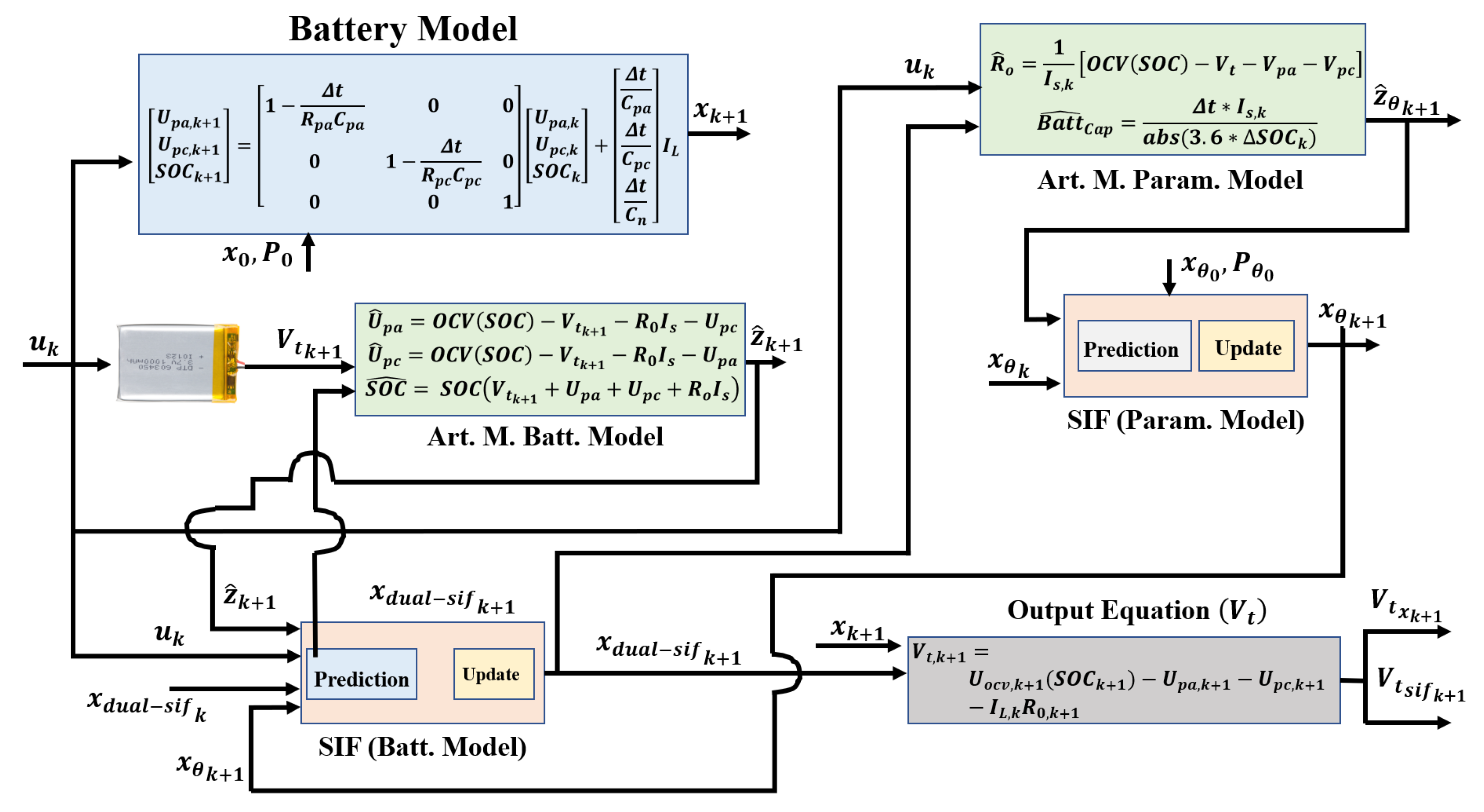
2. Battery Models
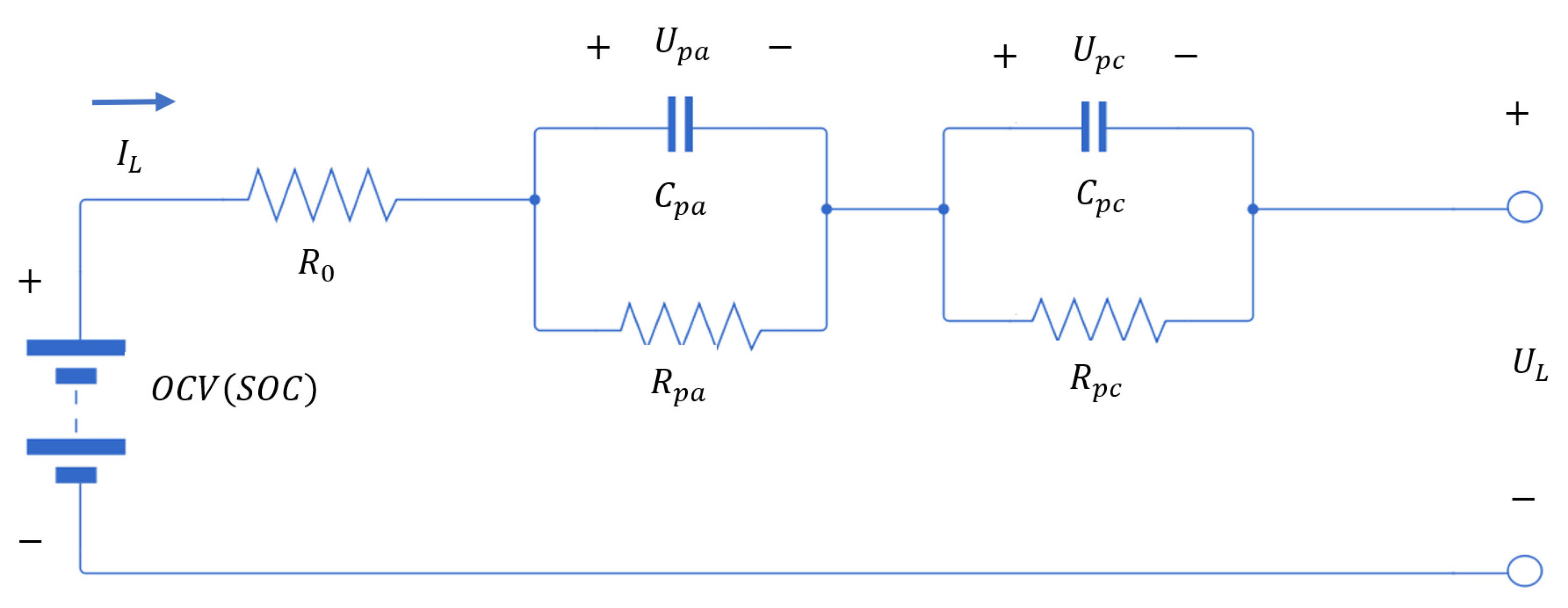
2.1. Dual Polarity Model
2.2. Parameter Model
3. Experimental Dataset and Estimation Methods
3.1. B005 Dataset
3.2. Ampere Hour Counting
3.3. Kalman Filter (KF)
3.4. Sliding Innovation Filter
3.5. Dual Filters: Dual-KF and Dual-SIF
4. Artificial Measurements
4.1. State Measurement Equations
 ) is the inverse function of .
4.2. Parameter Measurement Equations
5. Parameter Identification
Least Squares
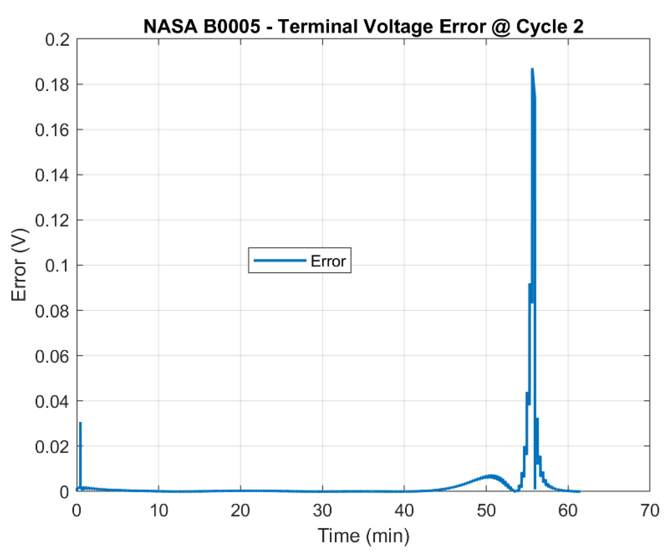
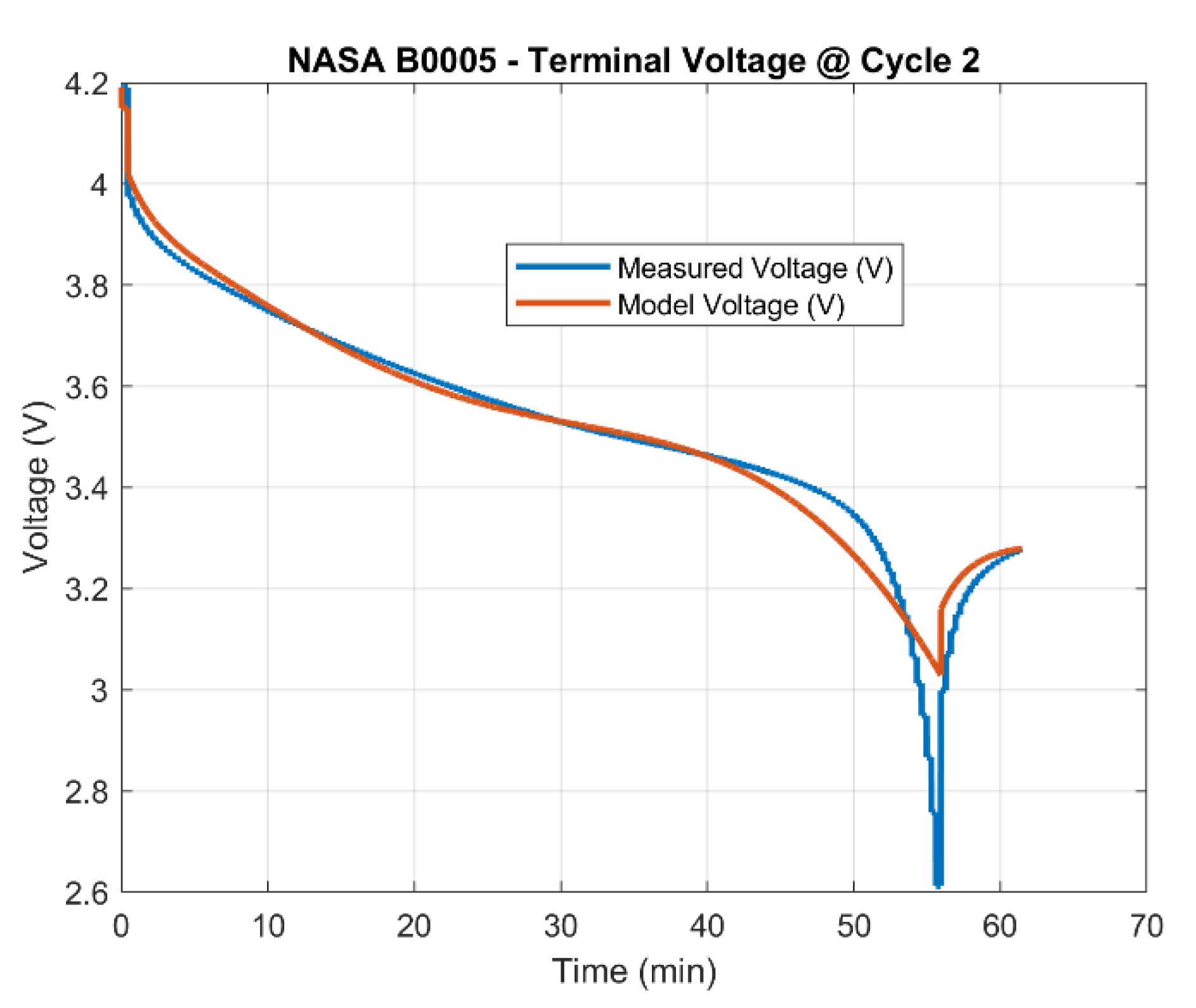
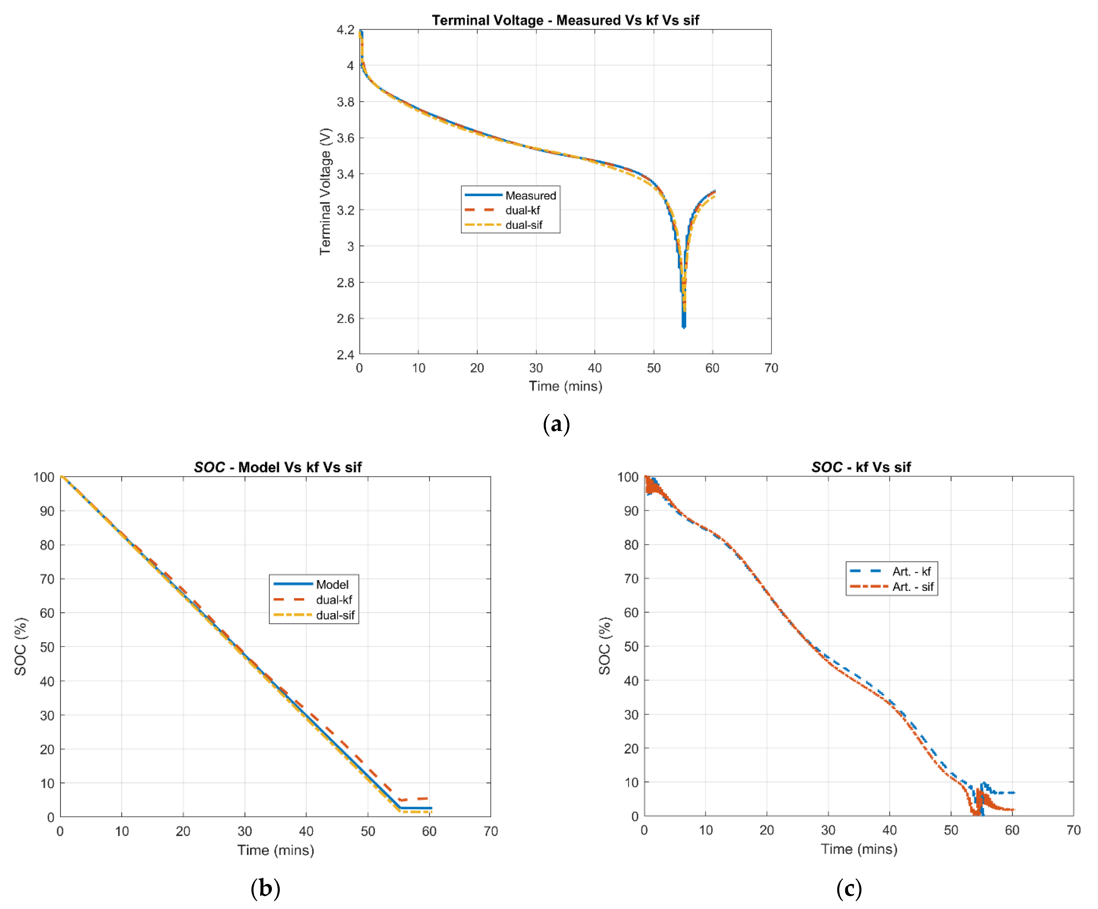
6. Experimental Results and Discussion
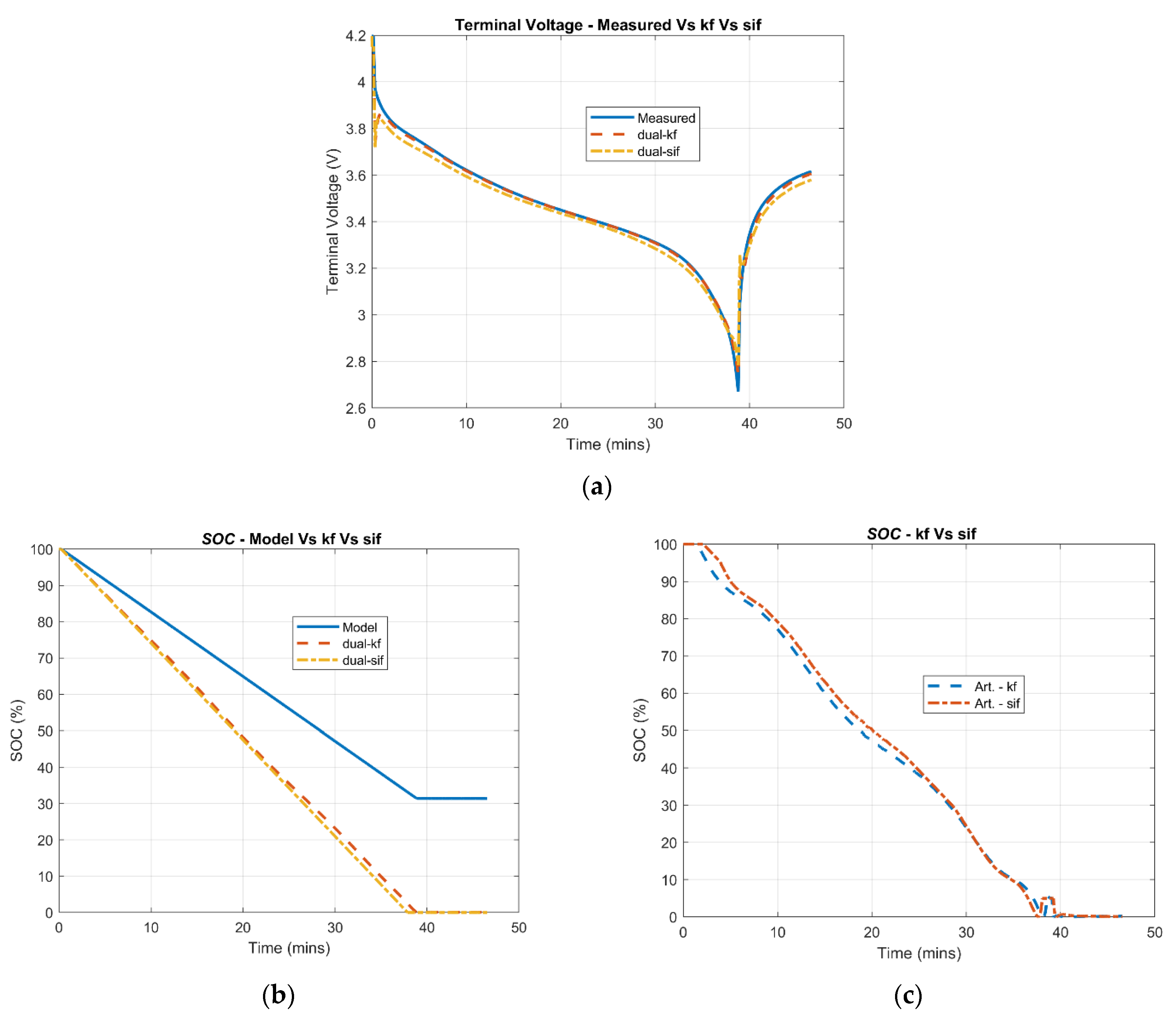
6.1. SOC Estimation: 10th Cycle and 400th Cycle
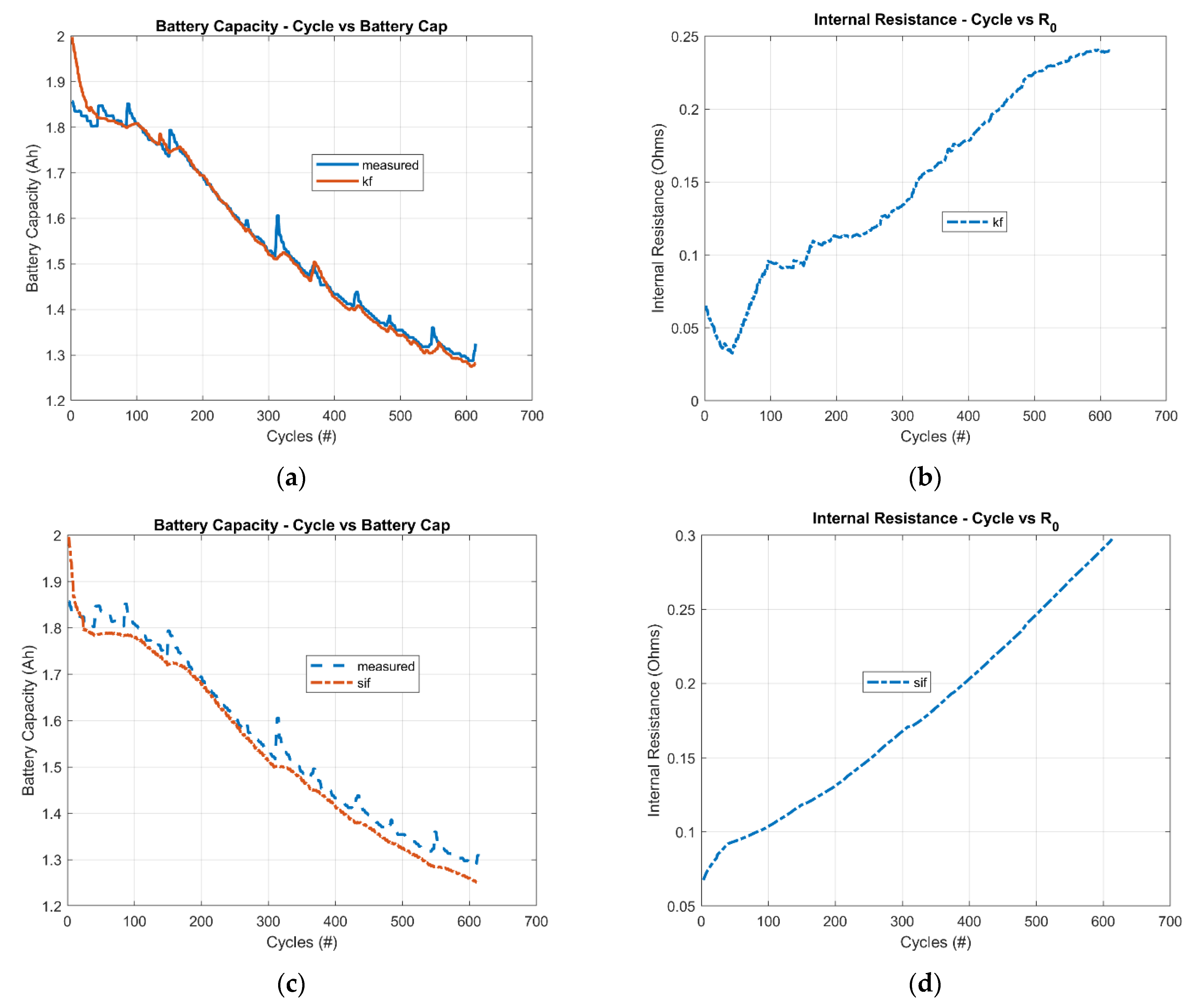
6.2. Battery Capacity Estimation: Dual KF and Dual SIF
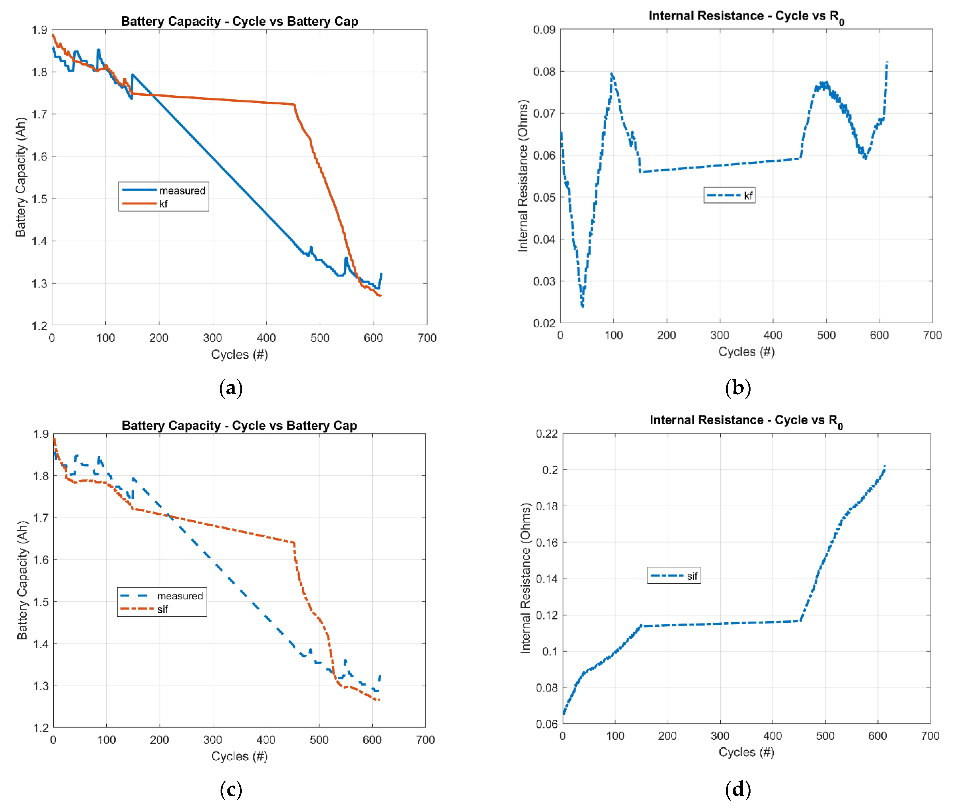
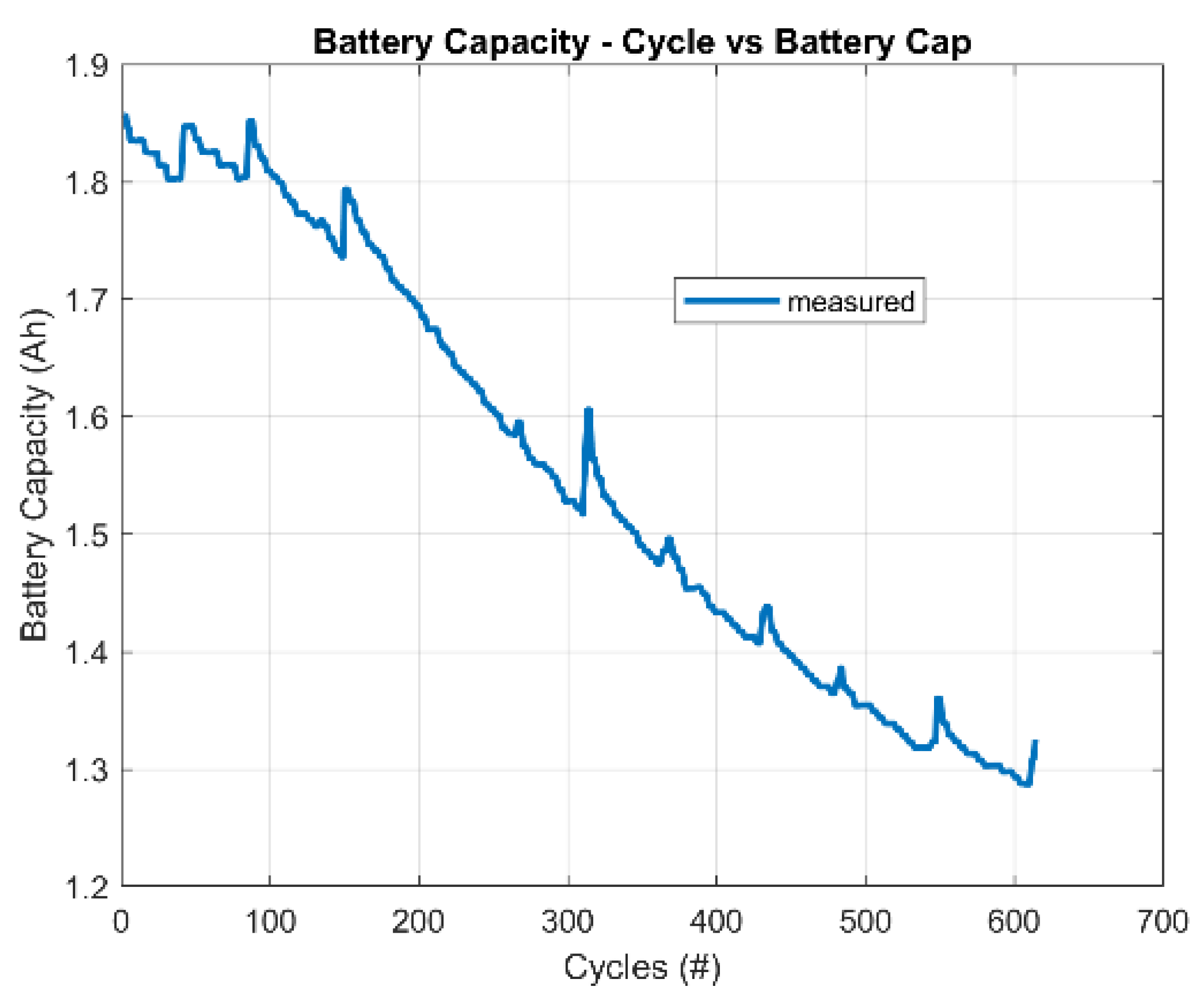
6.3. Battery Capacity Estimation under Fault: Jump in Data
7. Conclusions
Author Contributions
Funding
Institutional Review Board Statement
Informed Consent Statement
Data Availability Statement
Conflicts of Interest
References
- Li, X.; Sun, X.; Hu, X.; Fan, F.; Cai, S.; Zheng, C.; Stucky, G.D. Review on comprehending and enhancing the initial Coulombic efficiency of anode materials in lithium-ion/sodium-ion batteries. Nano Energy 2020, 77, 105143. [Google Scholar] [CrossRef]
- Zheng, L.; Zhu, J.; Wang, G.; Lu, D.D.-C.; He, T. Lithium-ion Battery Instantaneous Available Power Prediction Using Surface Lithium Concentration of Solid Particles in a Simplified Electrochemical Model. IEEE Trans. Power Electron. 2018, 33, 9551–9560. [Google Scholar] [CrossRef]
- IEEE Electronics Packing Society; Institute of Electrical and Electronics Engineers. Resistive Sensors Network Analog Multiplexing. In Proceedings of the 2018 IEEE 24th International Symposium for Design and Technology in Electronic Packaging (SIITME): IEEE Xplore Compliant Proceedings, Iasi, Romania, 25–28 October 2018; Institute of Electrical and Electronics Engineers: Piscataway, NJ, USA, 2018. ISBN 9781538655771. [Google Scholar]
- Nizam, H.M.; Maghfiroh, R.; Rosadi, A.; Kusumaputri, K.D.U. IEEE Staff. In Proceedings of the 2019 6th International Conference on Electric Vehicular Technology (ICEVT), Bali, Indonesia, 18–21 November 2019; IEEE: Piscataway, NJ, USA, 2019. ISBN 9781728129174. [Google Scholar]
- Ouyang, D.; Weng, J.; Chen, M.; Liu, J.; Wang, J. Experimental analysis on the degradation behavior of overdischarged lithium-ion battery combined with the effect of high-temperature environment. Int. J. Energy Res. 2020, 44, 229–241. [Google Scholar] [CrossRef]
- Feng, L.; Ding, J.; Han, Y. Improved sliding mode based EKF for the SOC estimation of lithium-ion batteries. Ionics 2020, 26, 2875–2882. [Google Scholar] [CrossRef]
- Zhang, S.; Sun, H.; Lyu, C. A method of SOC estimation for power Li-ion batteries based on equivalent circuit model and extended Kalman filter. In Proceedings of the 2018 13th IEEE Conference on Industrial Electronics and Applications (ICIEA), Wuhan, China, 31 May–2 June 2018; Institute of Electrical and Electronics Engineers Inc.: Piscataway, NJ, USA, 2018; pp. 2683–2687. [Google Scholar]
- Luo, J.; Peng, J.; He, H. Lithium-ion battery SOC estimation study based on Cubature Kalman filter. Energy Procedia 2019, 158, 3421–3426. [Google Scholar] [CrossRef]
- He, H.; Qin, H.; Sun, X.; Shui, Y. Comparison Study on the Battery SoC Estimation with EKF and UKF Algorithms. Energies 2013, 6, 5088–5100. [Google Scholar] [CrossRef]
- How, D.N.T.; Hannan, M.A.; Hossain Lipu, M.S.; Ker, P.J. State of Charge Estimation for Lithium-Ion Batteries Using Model-Based and Data-Driven Methods: A Review. IEEE Access 2019, 7, 136116–136136. [Google Scholar] [CrossRef]
- Westerhoff, U.; Kurbach, K.; Lienesch, F.; Kurrat, M. Analysis of Lithium-Ion Battery Models Based on Electrochemical Impedance Spectroscopy. Energy Technol. 2016, 4, 1620–1630. [Google Scholar] [CrossRef] [Green Version]
- Tran, N.-T.; Khan, A.B.; Nguyen, T.-T.; Kim, D.-W.; Choi, W. SOC Estimation of Multiple Lithium-Ion Battery Cells in a Module Using a Nonlinear State Observer and Online Parameter Estimation. Energies 2018, 11, 1620. [Google Scholar] [CrossRef] [Green Version]
- Lai, X.; Qiao, D.; Zheng, Y.; Zhou, L. A Fuzzy State-of-Charge Estimation Algorithm Combining Ampere-Hour and an Extended Kalman Filter for Li-Ion Batteries Based on Multi-Model Global Identification. Appl. Sci. 2018, 8, 2028. [Google Scholar] [CrossRef] [Green Version]
- Institute of Electrical and Electronics Engineers. Predictive Method of Capacitor Production Order Based on ARIMA Model. In Proceedings of the 2018 IEEE 4th International Conference on Control Science and Systems Engineering (ICCSSE), Wuhan, China, 21–23 August 2018; IEEE: Piscataway, NJ, USA, 2018. ISBN 9781538678879. [Google Scholar]
- Zhang, C.; Li, K.; Mcloone, S.; Yang, Z. Battery modelling methods for electric vehicles—A review. In Proceedings of the 2014 European Control Conference (ECC), Strasbourg, France, 24–27 June 2014; Institute of Electrical and Electronics Engineers Inc.: Piscataway, NJ, USA, 2014; pp. 2673–2678. [Google Scholar]
- Vehicular Technology Society; Truòng đại học bách khoa Hà Nôi; Institute of Electrical and Electronics Engineers. Connect green e-Motion. In Proceedings of the 2019 IEEE Vehicle Power and Propulsion Conference (VPPC), Hanoi, Vietnam, 14–17 October 2019; IEEE: Piscataway, NJ, USA, 2019. ISBN 9781728112497. [Google Scholar]
- He, H.; Xiong, R.; Fan, J. Evaluation of Lithium-Ion Battery Equivalent Circuit Models for State of Charge Estimation by an Experimental Approach. Energies 2011, 4, 582–598. [Google Scholar] [CrossRef]
- Eltoumi, F.; Badji, A.; Becherif, M.; Ramadan, H.S. Experimental Identification using Equivalent Circuit Model for Lithium-Ion Battery. Int. J. Emerg. Electr. Power Syst. 2018, 19, 20170210. [Google Scholar] [CrossRef]
- Song, Y.; Park, M.; Seo, M.; Kim, S.W. Improved SOC estimation of lithium-ion batteries with novel SOC-OCV curve estimation method using equivalent circuit model. In Proceedings of the 2019 4th International Conference on Smart and Sustainable Technologies (SpliTech), Split, Croatia, 18–21 June 2019. [Google Scholar]
- China Power Supply Society; IEEE Power Electronics Society; Power Sources Manufacturers Association; Institute of Electrical and Electronics Engineers. The state-of-the-art in power electronics, energy conversion and its applications. In Proceedings of the 2018 IEEE International Power Electronics and Application Conference and Exposition (PEAC), Crowne Plaza Shenzhen Longgang City Centre, Shenzhen, China, 4–7 November 2018; IEEE: Piscataway, NJ, USA, 2018. ISBN 9781538660546. [Google Scholar]
- Vidal, C.; Malysz, P.; Kollmeyer, P.; Emadi, A. Machine Learning Applied to Electrified Vehicle Battery State of Charge and State of Health Estimation: State-of-the-Art. IEEE Access 2020, 8, 52796–52814. [Google Scholar] [CrossRef]
- IEEE Control Systems Society; IEEE Robotics and Automation Society; Keisoku Jido Seigyo Gakkai (Japan); Institute of Electrical and Electronics Engineers. Proceedings of the First Annual IEEE Conference on Control Technology and Applications: CCTA 2017, Kohala Coast, HI, USA, 27–30 August 2017; IEEE: Piscataway, NJ, USA, 2017; ISBN 9781509021826. [Google Scholar]
- Xia, B.; Lao, Z.; Zhang, R.; Tian, Y.; Chen, G.; Sun, Z.; Wang, W.; Sun, W.; Lai, Y.; Wang, M.; et al. Online Parameter Identification and State of Charge Estimation of Lithium-Ion Batteries Based on Forgetting Factor Recursive Least Squares and Nonlinear Kalman Filter. Energies 2017, 11, 3. [Google Scholar] [CrossRef] [Green Version]
- Bezha, M.; Nagaoka, N. Online learning ANN model for SoC estimation of the Lithium- Ion battery in case of small amount of data for practical applications. In Proceedings of the 2019 10th International Conference on Power Electronics and ECCE Asia (ICPE 2019-ECCE Asia), Busan, Korea, 27–31 May 2019; IEEE: Piscataway, NJ, USA, 2019. [Google Scholar]
- Taborelli, C.; Onori, S. State of charge estimation using extended Kalman filters for battery management system. In Proceedings of the 2014 IEEE International Electric Vehicle Conference (IEVC), Florence, Italy, 17–19 December 2014; Institute of Electrical and Electronics Engineers Inc.: Piscataway, NJ, USA, 2014; pp. 1–8. [Google Scholar]
- Wielitzka, M.; Dagen, M.; Ortmaier, T. Joint unscented Kalman filter for state and parameter estimation in vehicle dynamics. In Proceedings of the 2015 IEEE Conference on Control Applications (CCA), Sydney, Australia, 21–23 September 2015; Institute of Electrical and Electronics Engineers Inc.: Piscataway, NJ, USA, 2015; pp. 1945–1950. [Google Scholar] [CrossRef]
- Erlangga, G.; Perwira, A.; Widyotriatmo, A. State of charge and state of health estimation of lithium battery using dual Kalman filter method. In Proceedings of the 2018 International Conference on Signals and Systems (ICSigSys), Bali, Indonesia, 1–3 May 2018; Institute of Electrical and Electronics Engineers Inc.: Piscataway, NJ, USA, 2018; pp. 243–248. [Google Scholar]
- Liao, Q.; Mu, M.; Zhao, S.; Zhang, L.; Jiang, T.; Ye, J.; Shen, X.; Zhou, G. Performance assessment and classification of retired lithium ion battery from electric vehicles for energy storage. Int. J. Hydrogen Energy 2017, 42, 18817–18823. [Google Scholar] [CrossRef]
- Hasib, S.A.; Islam, S.; Chakrabortty, R.K.; Ryan, M.J.; Saha, D.K.; Ahamed, H.; Moyeen, S.I.; Das, S.K.; Ali, F.; Islam, R.; et al. A Comprehensive Review of Available Battery Datasets, RUL Prediction Approaches, and Advanced Battery Management. IEEE Access 2021, 9, 86166–86193. [Google Scholar] [CrossRef]
- Lai, X.; Wang, S.; He, L.; Zhou, L.; Zheng, Y. A hybrid state-of-charge estimation method based on credible increment for electric vehicle applications with large sensor and model errors. J. Energy Storage 2020, 27, 101106. [Google Scholar] [CrossRef]
- Kalman, R.E. A New Approach to Linear Filtering and Prediction Problems. J. Basic Eng. 1960, 82, 35–45. [Google Scholar] [CrossRef] [Green Version]
- Welch, G.; Bishop, G. An Introduction to the Kalman Filter; ACM, Inc.: New York, NY, USA, 2001. [Google Scholar]
- Gadsden, S.A.; Habibi, S.; Kirubarajan, T. Kalman and smooth variable structure filters for robust estimation. IEEE Trans. Aerosp. Electron. Syst. 2014, 50, 1038–1050. [Google Scholar] [CrossRef]
- Gadsden, S.A.; Al-Shabi, M. The Sliding Innovation Filter. IEEE Access 2020, 8, 96129–96138. [Google Scholar] [CrossRef]
- Lee, A.S.; Gadsden, S.A.; Al-Shabi, M. An Adaptive Formulation of the Sliding Innovation Filter. IEEE Signal Process. Lett. 2021, 28, 1295–1299. [Google Scholar] [CrossRef]
- Nejad, S.; Gladwin, D.; Stone, D. A systematic review of lumped-parameter equivalent circuit models for real-time estimation of lithium-ion battery states. J. Power Sources 2016, 316, 183–196. [Google Scholar] [CrossRef] [Green Version]
- Wei, X.; Yimin, M.; Feng, Z. Lithium-ion Battery Modeling and State of Charge Estimation. Integr. Ferroelectr. 2019, 200, 59–72. [Google Scholar] [CrossRef]


| Parameters | |||||
|---|---|---|---|---|---|
| Unit | 1/() | 1/() | |||
| LB | 0.001 | 0.01 | 0.0001 | 0.01 | 0.01 |
| UB | 0.500 | 0.50 | 0.0020 | 0.50 | 0.10 |
| Guess | 0.020 | 0.10 | 0.0010 | 0.10 | 0.01 |
| RC-Parameters | Value | OCV(SOC) | Value |
|---|---|---|---|
| 0.065 | 2.94 | ||
| 0.0615 | −5.66 | ||
| 1860 | 2.70 | ||
| 0.0227 | 3.84 | ||
| 146825 | −2.94 |
| Variable | Battery Model | Parameter Model |
|---|---|---|
| 0 | 0.065 | |
| 0 | 2 Ah | |
| SOC | 100% | - |
| Diag (5 × 10⁻⁵, 3 × 10⁻⁵, 5 × 10⁻⁷) | Diag (5 × 10⁻⁷, 1 × 10⁻⁸) | |
| Diag (0.1, 0.01, 1) | Diag (10, 1) | |
| Delta | [10; 7; 2000] | [450; 90] |
| Output/State | Dual-KF | Dual-SIF |
|---|---|---|
| 0.0283 | 0.0342 | |
| Terminal Voltage | 0.0227 | 0.0398 |
| Output/State | Dual-KF | Dual-SIF |
|---|---|---|
| Batcap | 0.1233 | 0.0675 |
| Terminal Voltage | 0.0776 | 0.0460 |
Publisher’s Note: MDPI stays neutral with regard to jurisdictional claims in published maps and institutional affiliations. |
© 2022 by the authors. Licensee MDPI, Basel, Switzerland. This article is an open access article distributed under the terms and conditions of the Creative Commons Attribution (CC BY) license (https://creativecommons.org/licenses/by/4.0/).
Share and Cite
Bustos, R.; Gadsden, S.A.; Malysz, P.; Al-Shabi, M.; Mahmud, S. Health Monitoring of Lithium-Ion Batteries Using Dual Filters. Energies 2022, 15, 2230. https://doi.org/10.3390/en15062230
Bustos R, Gadsden SA, Malysz P, Al-Shabi M, Mahmud S. Health Monitoring of Lithium-Ion Batteries Using Dual Filters. Energies. 2022; 15(6):2230. https://doi.org/10.3390/en15062230
Chicago/Turabian StyleBustos, Richard, Stephen Andrew Gadsden, Pawel Malysz, Mohammad Al-Shabi, and Shohel Mahmud. 2022. "Health Monitoring of Lithium-Ion Batteries Using Dual Filters" Energies 15, no. 6: 2230. https://doi.org/10.3390/en15062230
APA StyleBustos, R., Gadsden, S. A., Malysz, P., Al-Shabi, M., & Mahmud, S. (2022). Health Monitoring of Lithium-Ion Batteries Using Dual Filters. Energies, 15(6), 2230. https://doi.org/10.3390/en15062230