A Convolutional Neural Network Approach for Estimation of Li-Ion Battery State of Health from Charge Profiles

Abstract

Intelligent and pragmatic state-of-health (SOH) estimation is critical for the safe and reliable operation of Li-ion batteries, which recently have become ubiquitous for applications such as electrified vehicles, smart grids, smartphones, as well as manned and unmanned aerial vehicles. This paper introduces a convolutional neural network (CNN)-based framework for directly estimating SOH from voltage, current, and temperature measured while the battery is charging. The CNN is trained with data from as many as 28 cells, which were aged at two temperatures using randomized usage profiles. CNNs with between 1 and 6 layers and between 32 and 256 neurons were investigated, and the training data was augmented with noise and error as well to improve accuracy. Importantly, the algorithm was validated for partial charges, as would be common for many applications. Full charges starting between 0 and 95% SOC as well as for multiple ranges ending at less than 100% SOC were tested. The proposed CNN SOH estimation framework achieved a mean average error (MAE) as low as 0.8% over the life of the battery, and still achieved a reasonable MAE of 1.6% when a very small charge window of 85% to 97% SOC was used. While the CNN algorithm is shown to estimate SOH very accurately with partial charge data and two temperatures, further studies could also investigate a wider temperature range and multiple different charge currents or constant power charging.

1. Introduction

Like most things, Li-ion batteries age with time; a process underpinned by the degradation of electrode materials, loss of lithium in active carbon, lithium metal plating and chemical decomposition, to name a few. If aging is not correctly monitored, an accurate estimate of available battery capacity is not possible, which greatly compromises a battery’s safety and reliability.

Battery aging is typically determined through a state-of-health (SOH) estimation which has a value ranging between 0 and 100%. For this work, SOH is defined as the ratio of aged and new capacity of the battery. In some industries, such as the automotive industry, the standard for end of life of a Li-ion battery is when SOH = 80% is reached [1]. SOH is not an observable quantity and is a highly nonlinear entity, dependent, in large part, on the volatility of the loading profiles, ambient temperature, depth of discharge (DOD) and self-discharge, to name a few [2]. Therefore, an accurate estimate of SOH is typically a tedious computation.

It is difficult for a battery model to capture all the underlying electrochemical processes and provide accurate estimates of SOH. The benefit of data-driven methods is that they rely mainly on aging data, therefore they do not require knowledge of these underlying processes, and in some cases, they also avoid using a physical model. In [3], the authors capitalize on the correlation between the diffusion capacitance of a second-order equivalent circuit model and state of health. A genetic algorithm (GA) is used to estimate the voltage drop across the diffusion capacitance as well as to estimate the open circuit voltage. The maximum error observed while using this estimation strategy is 4.35%. In [4], after a three-dimensional OCV-SOC surface spanning the lifetime of the battery was generated, the capacity and initial SOC of the battery were computed based on a GA and an equivalent circuit model (ECM). The estimation error of this technique ranges between 1.09–4.52%, depending on the test case used. Aside from GA, other works have used particle swarm optimization (PSO) to ascertain battery aging parameters [5,6].

Recently, due to the increased number of publicly available battery datasets, machine learning techniques are gaining popularity for battery state estimation. Algorithms have been investigated including support vector machines, least-squared support vector machines, K-nearest regression, radial basis functions, random forest, Bayesian networks; feed-forward, deep, convolutional, Hamming, and recurrent neural networks, as outlined in review papers [7,8]. In one example, battery cycle life is predicted early in the life of the battery by using machine learning with inputs including measured data and calculated features, such as the change in amp hours with respect to voltage (dQ/dV) [9]. Several studies specifically investigated different ways of utilizing convolutional neural networks (CNNs) for battery state-of-health estimation. A CNN is trained to estimate battery capacity from the measured impedance and state of charge values in [10]. In [11], a CNN and a relevance vector machine were both compared for SOH estimation. A CNN is combined with a gated recurrent neural network in [12] and two CNNs are used with random forest in [13], with both combinations showing improved SOH estimation. Finally, a different method of sampling data, at fixed SOC steps rather than fixed time steps, was shown to be beneficial for battery SOH estimation with a CNN, FNN, or LSTM [14].

In [15], battery current, voltage and temperature are recorded during a particular window of operation of the battery and used to train a support vector machine (SVM). The SVM is used as a battery model to estimate capacity or resistance of the battery and achieves around 0.1 Ah accuracy. However, when applied in real world scenarios, training an SVM using measured battery signals on board the vehicle can result in large errors as a result of noisy measurement devices. In [16], electrochemical impedance spectroscopy (EIS) measurements are used to construct an equivalent circuit model of a battery. Then, a recurrent neural network takes as inputs historical values of SOC, current, resistance and capacitance and outputs future values of capacitance and resistance parameters of the model. The method achieves a mean squared error 0.462 Ah. The drawback of this method is that it still requires a battery model, one generated using the harder-to-obtain EIS measurements. In addition, vanilla recurrent neural networks commonly suffer from vanishing gradients and thus can be difficult to train.

In [17], the probability density function (PDF) of the terminal voltage of a discharge profile is used to estimate the battery SOH. The strategy maps the peak values of a smoothed PDF profile to SOH values. The study achieves an error of below 1.6% on the reference charge curves, however, its performance over partial reference profiles, often encountered in real world scenarios, is unknown.

Since discharge profiles observed between charging events occur in an uncontrolled fashion, some works have relied on charge profiles to estimate SOH. In [18,19], incremental capacity analysis (ICA) profiles, described as dQ/dV, are used to detect small incremental changes in the charge curves. To identify this ICA profile from noisy measurements and from partial reference profiles, a support vector machine showed the best results in [18]. This method achieves a 1% mean absolute error (MAE), however, to identify the ICA curve from noisy measurement data, it is necessary to make use of support vector machines, which is an additional intermittent step that adds computational overhead and reduces the generalizability of the method. In [20], the constant current component of the charging voltage curve is used with an equivalent circuit model to extract the aging parameters. Parameter identification is achieved using a nonlinear least squares technique. This work achieves 2–3% errors, however, its performance is based on full charge profiles and not on more realistic partial charge curves. The battery in an EV is very rarely fully discharged down to SOC = 0%, hence, the battery is typically charged from some SOC greater than 0%. In other words, the battery undergoes partial charge profiles much more frequently than full charge profiles.

This work uses a CNN, a well-known deep learning algorithm, to estimate SOH. Specifically, there are three main contributions in this work:

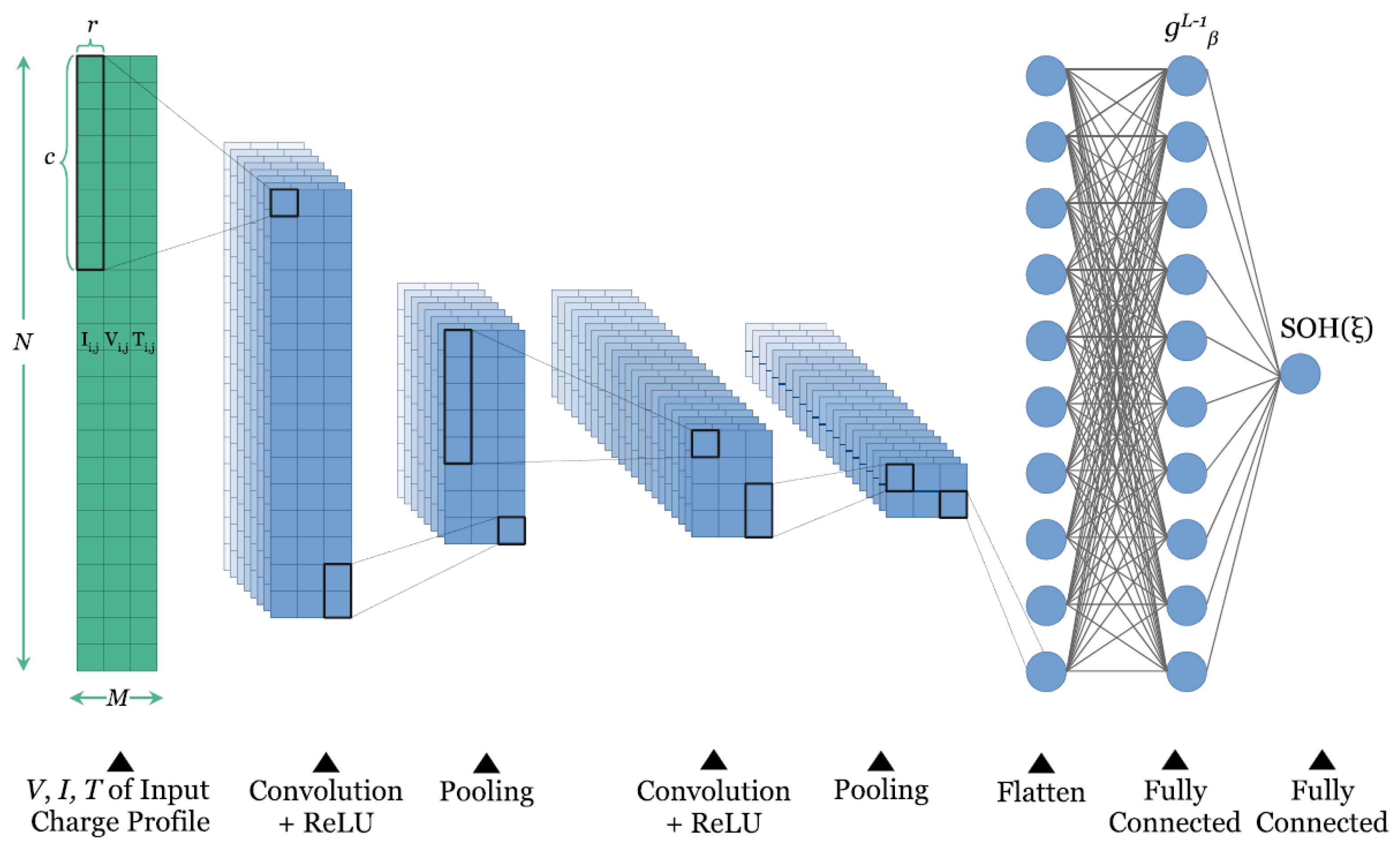
• A CNN is used to map raw battery measurements directly to SOH without the use of any physical or electrochemical models. The performance of the CNN is not limited by knowledge of the underlying electrochemical processes. Physical or electrochemical models are more challenging to create because they must include complex processes such as self-discharge, solid lithium concentrations, etc.
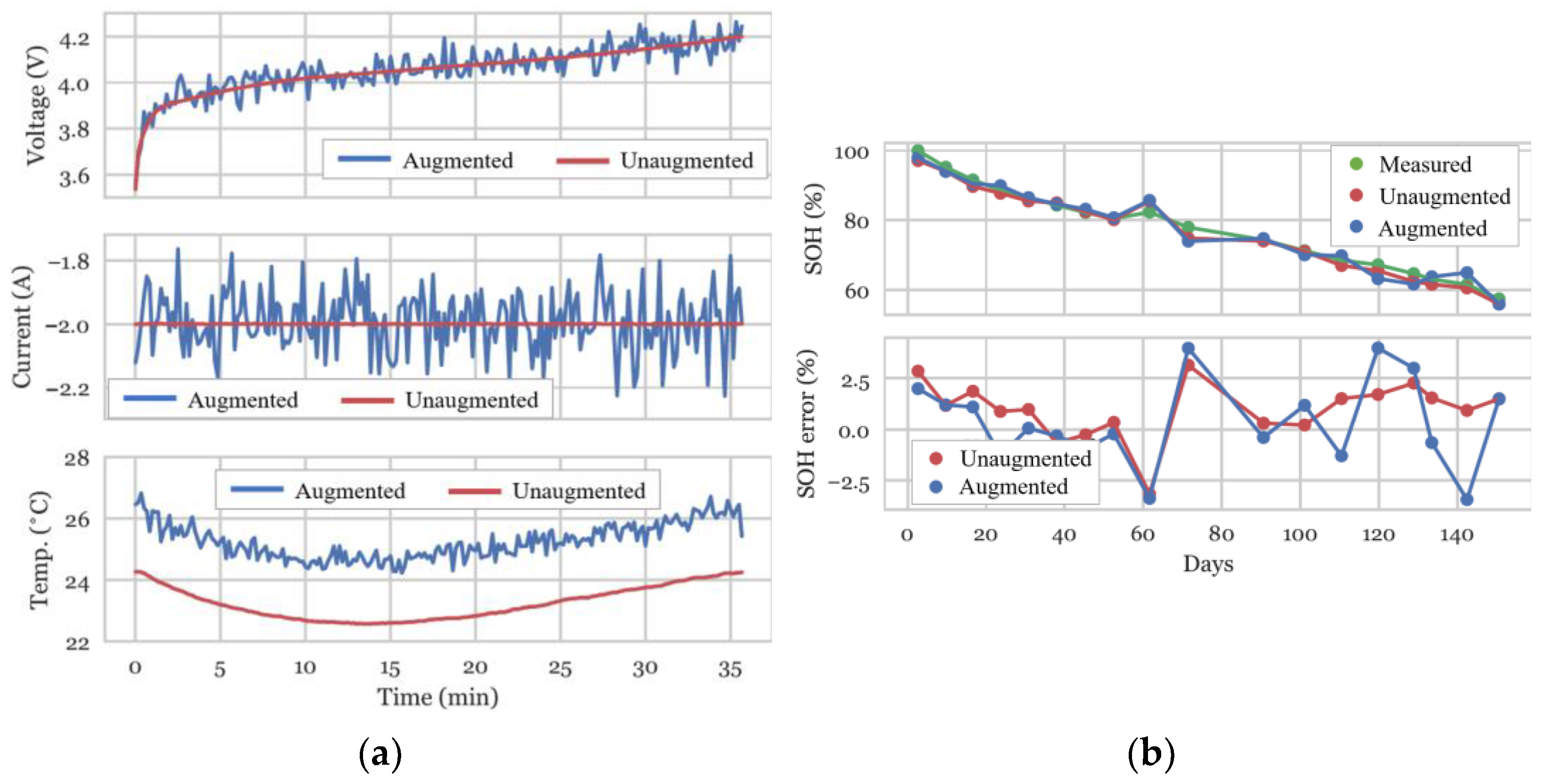
• A data augmentation technique is used to generate the training data used as inputs to the CNN. This not only makes the CNN more robust against measurement noise, offsets and gains but also increases the CNN’s SOH estimation accuracy.
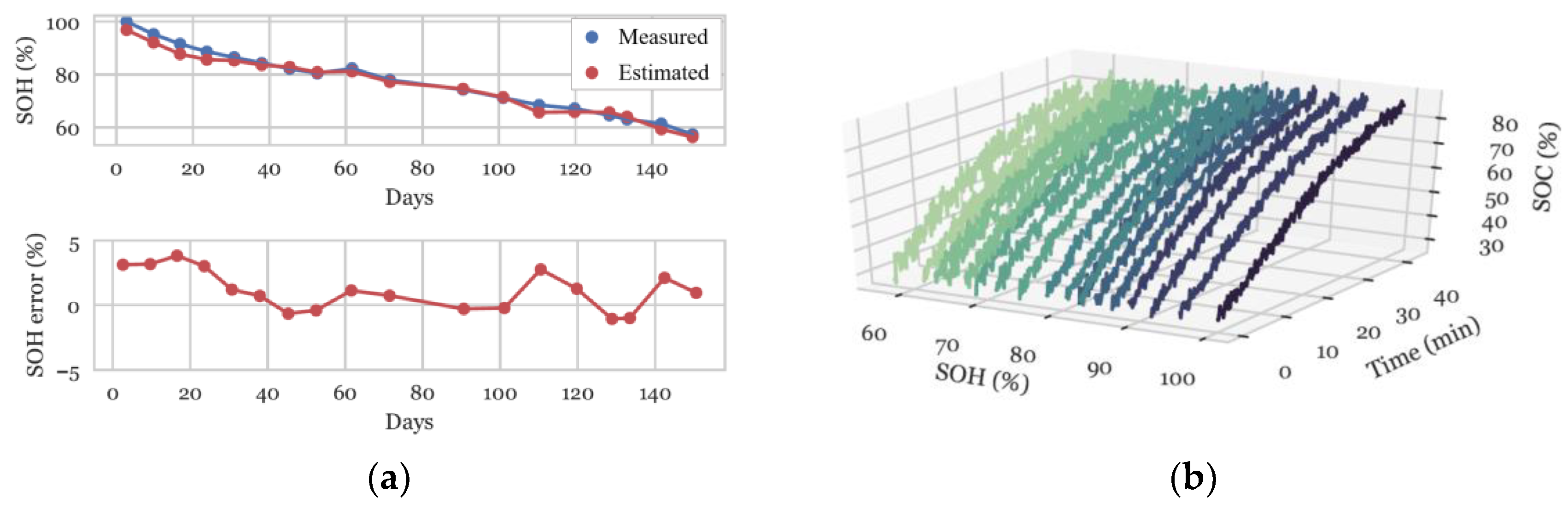
• To further increase the CNN’s practicality in real-world applications, it is trained to estimate SOH over partial charge profiles having varying ranges of state of charge (SOC). This is an important feature increasing the practicality of this method considerably.

The second section of the paper focuses on the theoretical underpinnings of the CNN algorithm and the third section discusses the randomized usage aging dataset obtained from the NASA repository [21] as well as the CNN model development using this dataset. The fourth section discusses the results.

2. Background and Theory of Convolutional Neural Networks for SOH Estimation

Lately, the surge of interest in artificial intelligence (AI) has been primarily underpinned by the numerous advancements achieved in deep learning algorithms [22,23,24]. Although traditional machine learning methods have been studied for decades, advancements in computing power and an abundance of real-world data have allowed for much larger or deeper architectures. These new, deeper models have allowed for remarkable achievements within the field of artificial intelligence [25,26,27,28,29] as well as in other fields [30,31,32,33].

Convolutional neural networks, shown in Figure 1, are particularly good at mapping a set of measured quantities to a desired output. The CNNs used in this work convolve filters over the input, passing the result to the next layer instead of fully interconnected adjacent layers as is typically done in fully connected neural networks. Convolving filters over the two-dimensional dataset allow these networks to benefit from shared weights and an invariance to local distortions [24]. The CNN’s filters look at data from multiple time steps during a convolution operation which includes the data point at the present time step as well as some amount of historical data points. Because of shared weights, CNNs can be given a large amount of input data without size increasing as much as for a fully connected neural network. Once CNNs are trained offline, they can offer fast computational speeds on board a mobile device or vehicle, since they are formulated by a series of convolution and matrix multiplication operations which can be computed in parallel. The typical dataset used for training and validation in this work is given by $D=\left\{\left(\Psi \left({\xi }_1\right),SO{H}^{*}\left({\xi }_1\right)\right),\dots ,\left(\Psi \left({\xi }_{\Xi }\right),SO{H}^{*}\left({\xi }_{\Xi }\right)\right)\right\}$, where $\Psi \left(\xi \right)$ and $SO{H}^{*}\left(\xi \right)$ are the array of input data and the ground-truth state-of-health values, respectively, for each charge profile, $\xi$. The input charge profiles, $\Psi \left(\xi \right)\in {ℝ}^{N\times M}$, which will be discussed further in the next section, can be composed of battery measurements such as current, voltage and temperature and, in the case of partial charge profiles, they also include the SOC values.

The kernel, $w^{lkm}$, is used in each layer of the CNN and has height $C_l$ and width $R_l$. The kernels are convolved over the input array of height $N_{l-1}$ and width $M_{l-1}$. For a more formal description, consider the element $x_{ij}^{lk}\left(\xi \right)$ at location $\left(k,j\right)$ in the kth feature map of layer l for charge profile $\xi$, given as follows;

$$\begin{gathered} x_{ij}^{lk}\left(\xi \right)=\eta \left({\displaystyle \sum }_m{\displaystyle \sum }_{c=0}^{C_l-1}{\displaystyle \sum }_{r=0}^{R_l-1}\left(w_{rc}^{lkm}{h}_{i+c,j+r}^{l-1,m}\left(\xi \right)+b^{lk}\right)\right) \\ {h}^{lk}\left(\xi \right)=S\left(x^{lk}\left(\xi \right)\right) \end{gathered}$$

(1)

where

$$\eta =\max \left(0,y\right)$$

(2)

In the above composite function, m is the feature map in layer l − 1, $b^{lk}$ is the bias for feature map k in layer l and $w_{rc}^{lkm}$ is the value of the kernel at the (c, r) location. $S\left(·\right)$ is a subsampling function, called max-pooling, which gives the maximum value of a perceived subset s of a feature map, where $\mathrm{s}\subseteq {\mathrm{h}}^{\mathrm{lk}}$.

The nonlinearity used in this work, η, is referred to as the rectified linear unit (ReLU). This is used in this work due to its simplicity and ease of implementation in real time. The last few layers of a CNN, as observed in Figure 1, are fully connected layers, formally described as follows;

$$g_{\beta }^l\left(\xi \right)=\eta \left({\displaystyle \sum }_{\beta }\left(w_{\alpha \beta }^l{h}_{\beta }^{l-1}\left(\xi \right)+b_{\beta }^l\right)\right)$$

(3)

where

$$g_{\mathsf{\beta }}^l\left(\mathsf{\xi }\right)=SOH\left(\mathsf{\xi }\right),\mathrm{for}l=L$$

(4)

and where $w_{\mathsf{\alpha }\mathsf{\beta }}^l$ denotes the weight connection between neuron α in the (l − 1)th layer and neuron β in the lth layer, $b_{\mathsf{\beta }}^l$ and $h_{\mathsf{\beta }}^l$ are the bias and activation function at layer l, respectively. The total number of layers in the CNN is given by L. To determine the SOH estimation performance of the CNN for a particular charge curve $\xi$, the estimated state of health, $SOH\left(\xi \right)$, is compared to the state-of-health ground-truth value, $SO{H}^{*}\left(\xi \right)$, resulting in an error value. The loss function is simply the mean squared error computed from all the individual errors, as follows;

$$ℒ=\frac{1}{\Xi }{\displaystyle \sum }_{\xi =0}^{\Xi }\left({\left(SOH\left(\xi \right)-SO{H}^{*}\left(\xi \right)\right)}^2\right)$$

(5)

where Ξ is the total number of charge curves in the training dataset.

One full training epoch, ϵ, describes a single cycle of one forward pass and one backward pass. In this work, training does not cease till a specified threshold criteria of loss is attained. In addition, the gradient of the loss function with respect to the weights is used to update the network weights in an optimization method called Adam [34]. This is given in the following composite function;

$$\begin{gathered} u_{ϵ}={\mathsf{\gamma }}_1{u}_{ϵ-1}\nabla ℒ\left(w_{ϵ-1}\right) \\ {v}_{ϵ}={\mathsf{\gamma }}_2{v}_{ϵ-1}\nabla ℒ{\left(w_{ϵ-1}\right)}^2 \\ \widetilde{u_{ϵ}}=u_{ϵ}/\left(1-{\mathsf{\gamma }}_1{}^{ϵ}\right) \\ \widetilde{v_{ϵ}}=v_{ϵ}/\left(1-{\mathsf{\gamma }}_2{}^{ϵ}\right) \\ {w}_{ϵ}=w_{ϵ-1}-\mathsf{\rho }\frac{\widetilde{u_{ϵ}}}{\widetilde{v_{ϵ}}-\mathsf{\kappa }}, \end{gathered}$$

(6)

where ${\gamma }_1$ and ${\mathsf{\gamma }}_2$ are decay rates set to 0.9 and 0.999, respectively, $\rho$ = 10⁻⁵ is the learning rate and $\mathsf{\kappa }$ is a constant term set to 10⁻⁸. The network weights at the present training epoch are given by $w_{ϵ}$. During the backward pass, the network self-learns its network weights and biases, a process referred to as backpropagation, which is a remarkable difference to other methods that demand time-consuming hand-engineered battery models and parameter identification. Validation, which in this paper refers to what is commonly considered testing, is performed on datasets which the CNN has never seen during training.

In this paper, state-of-health estimation performance was evaluated with various metrics. These include mean absolute error (MAE), root mean squared error (RMS), standard deviation of the errors (STDDEV) and the maximum error (MAX).

The CNN models discussed in this paper were created with TensorFlow, a machine learning framework. To expedite the training process two NVIDIA Graphical Processing Units (GPUs) were used, a TITAN X and a GeFORCE GTX 1080TI.

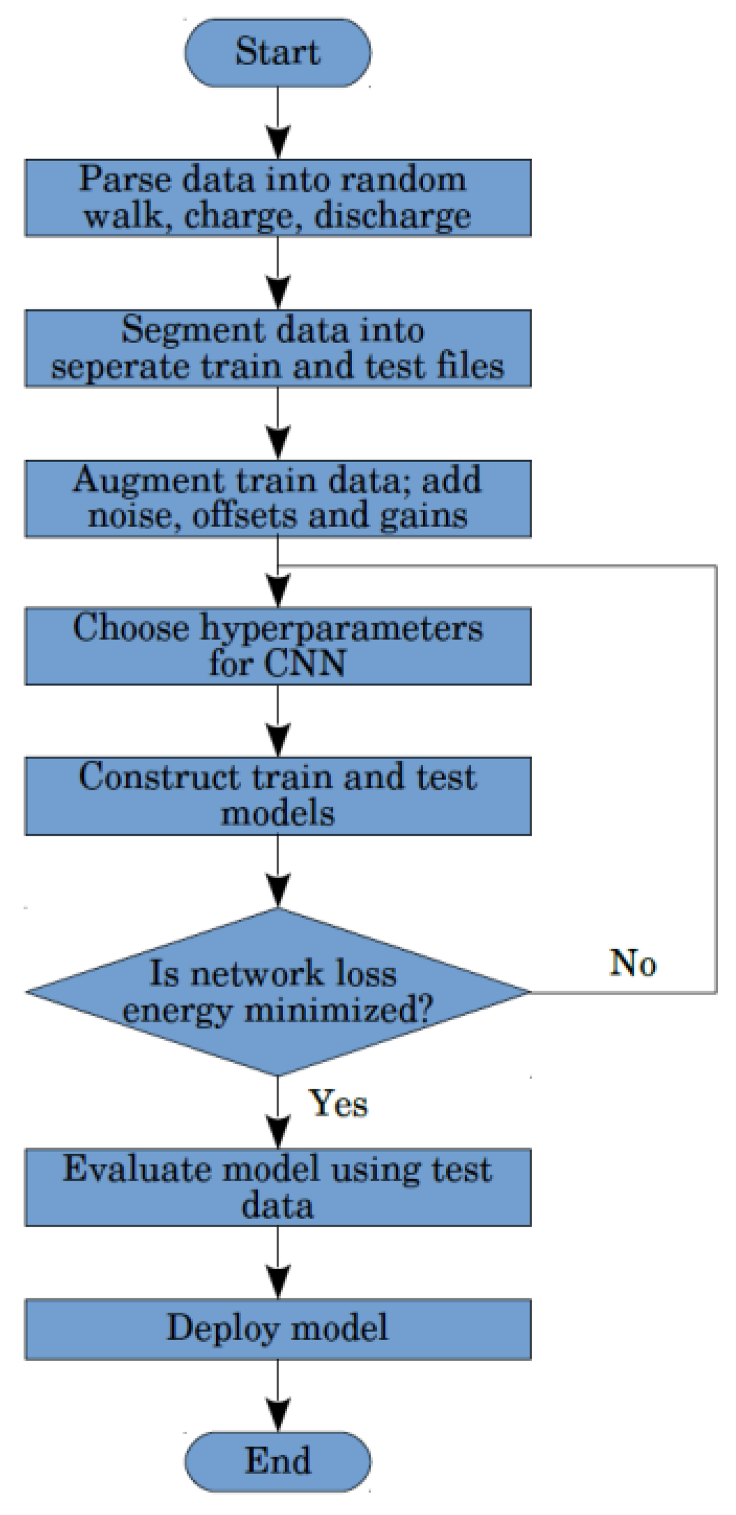
3. Methodology of Random Walk Aging Datasets and Data Preparation

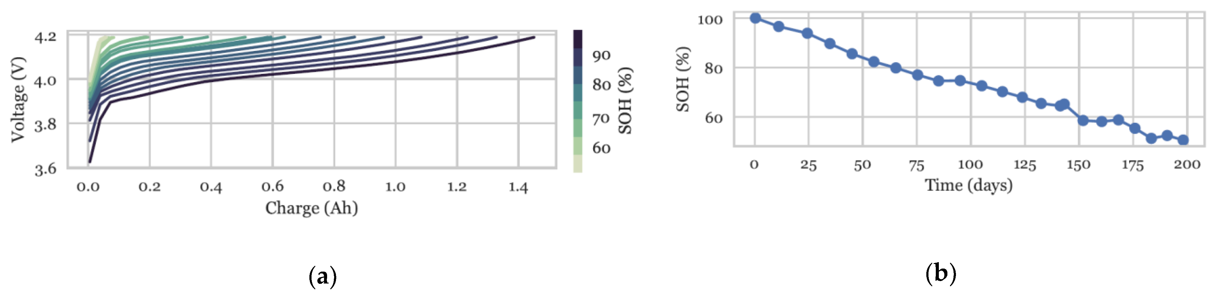
3.1. Randomized Battery Usage Datasets

The dataset used in this work is the Randomized Battery Usage Dataset obtained from the NASA Prognostics Center of Excellence [21]. The parameters of most of these datasets are shown in

Table 1. Randomized Battery Usage Dataset parameters.

Capacity @ SOH = 100%	Min. 2.08 Ah/Typ. 2.15 Ah
Min/Max Voltage	3.2 V/4.2 V
Min/Max Temperature	15 °C/43 °C
Charge Current (CC)	2.0 A
Random Walk Current	Min. −4.5 A/Max. 5.0 A

. The 28 LG Chem 18,650 Li-ion cells are aged by undergoing a randomized load; ranging between 0.5 A and 5 A for some datasets and −4.5 A to 4.5 A for others, often at different ambient temperatures. Each random walk step lasts for about 5 min. Random usage serves as a better representation of real-world loading profiles where vehicle acceleration and deceleration are unpredictable. Reference charge profiles were conducted roughly every 5 days to characterize the cell’s aging. These were sampled at 0.1 Hz, although this was not always consistent, and, as is typically performed, the charge curves in these characterization steps included a constant current (CC) and constant voltage (CV) segment. The CC segment of the charge profile was set to 2 A and typically consisted of the first 60 to 70% of the charge.

This work considers the fixed and partial SOC ranges where both the CC and the CV segments of the charge curves are utilized. For most of the 28 aging datasets in this repository, the cells are aged to at least SOH equal to 80% and in some cases to SOH less than 40%. An example of one aging dataset is shown in Figure 2, where, as the battery aged, the relationship of charging voltage to amp hours of charge added to the battery changed due to reduced capacity and increased impedance of the battery.

3.2. Data Processing

The entire process from data parsing to training and validation of the CNN are represented in a flowchart in Figure 3. The following was performed for every one of the 28 datasets of the repository. First, the reference charge profiles are extracted from the raw data. For example, dataset 1 of the 28 datasets, contains 40 reference charge profiles, spanning the entire lifetime of the aged battery cell. These are extracted and saved for the preprocessing step. Second, in the preprocessing step, the current voltage and temperature sequences of dataset 1 are resampled using linear interpolation at 0.1 Hz to ensure good discretization. The three signal sequences are concatenated together to form an array having 3 columns and 256 rows. Therefore, as shown in Figure 1, an input reference profile is defined as $\Psi \left(\xi \right)\in {ℝ}^{N\times M}$ where N = 256 and M = 3. Although we truncated the datasets to the first 256 time steps, the reference profiles were typically at least 1000 time steps long. For the case of the partial reference profiles, not only were the first 256 time steps selected but different segments of 256 time steps were also chosen throughout the full reference profile.

The number of rows is typically longer than 256, but we truncated the number of rows so that all reference profiles had the same duration in time. This was done to increase data impartiality; in other words, to avoid biasing the model towards reference profiles which might have had more time steps or which had a longer time span. The reference profiles for one dataset were then all concatenated depthwise to form a three-dimensional array. For example, in the case of dataset 1 containing 40 recorded reference profiles, the resulting dimensions after processing would be $256\times 3\times 40$.

The data points representing current during charging were multiplied by the sampling period of 10 s or 0.002778 h which were then summed to get the resulting capacity. This calculation was performed whenever the reference profiles were observed which was roughly every 5 days. To get the ground-truth SOH, the Ah calculation from all the reference profiles was divided by the Ah calculation conducted for the first observed reference profile, before any aging was performed.

3.3. Training Data Augmentation

The convolutional neural network is made more robust against noise, offsets and gains existent in real-world measurement devices by augmenting the training data. In this paper, a novel data augmentation technique was used by injecting Gaussian noise into the measured battery signals. Specifically, Gaussian noise with 0 mean and a standard deviation of 1–4% was injected into the voltage, current and temperature measurements. Moreover, to provide robustness against offsets and gains inherent in battery measurement devices, an offset was applied to all measurement signals and a gain was applied only to the current measurement since current measurements are more susceptible to gains. An offset of up to ±150 mA and a gain of up to ±3% was applied to the current measurements, an offset of up to ±5 mV was applied to the voltage measurement and an offset of up to ±5 °C was applied to the temperature measurement. Alternate copies of the training data were created with varying levels of noise, offsets and gains within the limits described above.

Before training and during the data augmentation step, up to 80 variants were created for each original dataset which would mean that 2240 datasets were used for the training. The noise, offset, and gain values used in the paper are similar to or are somewhat worse than those values seen for typical automotive sensors [35,36,37]. For example, a commercial grade current sensor may be rated for 0.5% noise on the output. A larger noise magnitude was selected in this paper than that inherent in many of these sensors for two reasons: (1) to help with the training of the network and reduce overfitting as well as to increase estimation accuracy; and (2) to emulate noise which may be injected into the system due to noisy power electronics or other EMI and EMC emitting equipment in an actual vehicle.

This data augmentation technique is inspired by a method sometimes referred to as jittering [38,39] which not only makes the model more robust against measurement error but it also leads to higher estimation accuracies and reduces overfitting. After training on this augmented data, we also tested the model on augmented test data which was intentionally injected with signal error to test the CNN’s robustness.

4. State of Health Estimation Results and Discussion

The state-of-health estimation performance of the deep convolutional networks are outlined in this section. As previously mentioned, this work used charge profiles which included both fixed (beginning at SOC = 0%) and partial SOC ranges (beginning at SOC > 0%). There are trade-offs which need to be made in either case and these will be discussed in the following two sections. The results obtained over full reference charge profiles serve as a good baseline to which the performance over partial charge profiles can be compared. The networks discussed in this section used a learning rate of $1\times {10}^{-5}$.

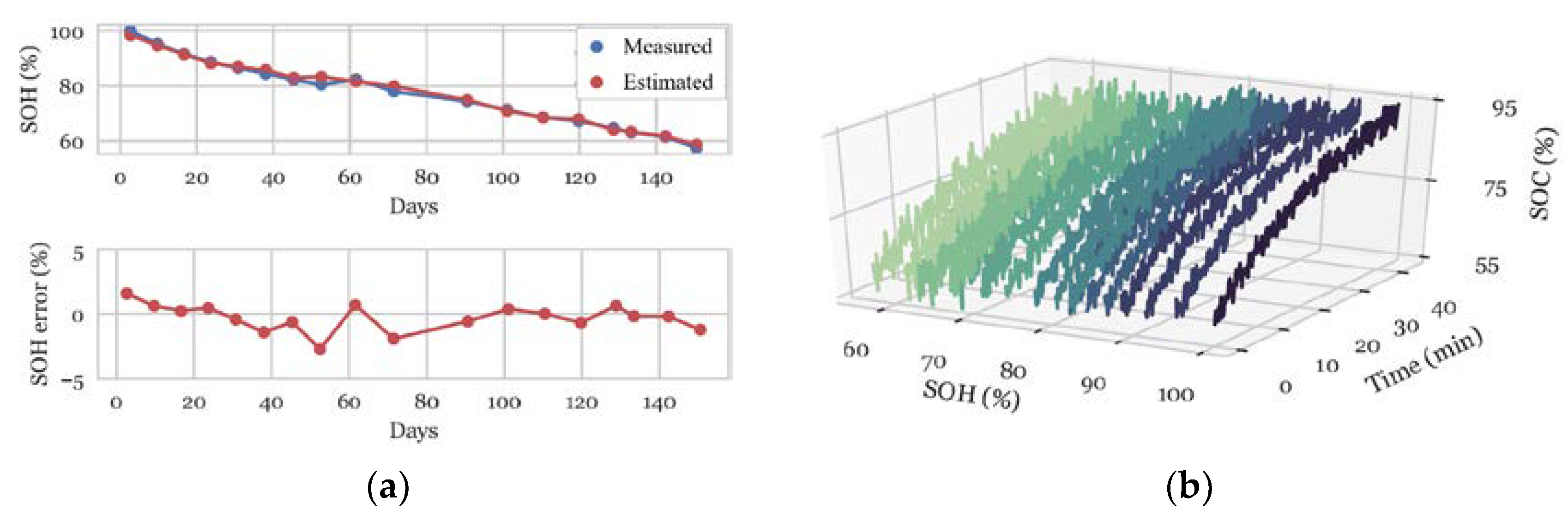
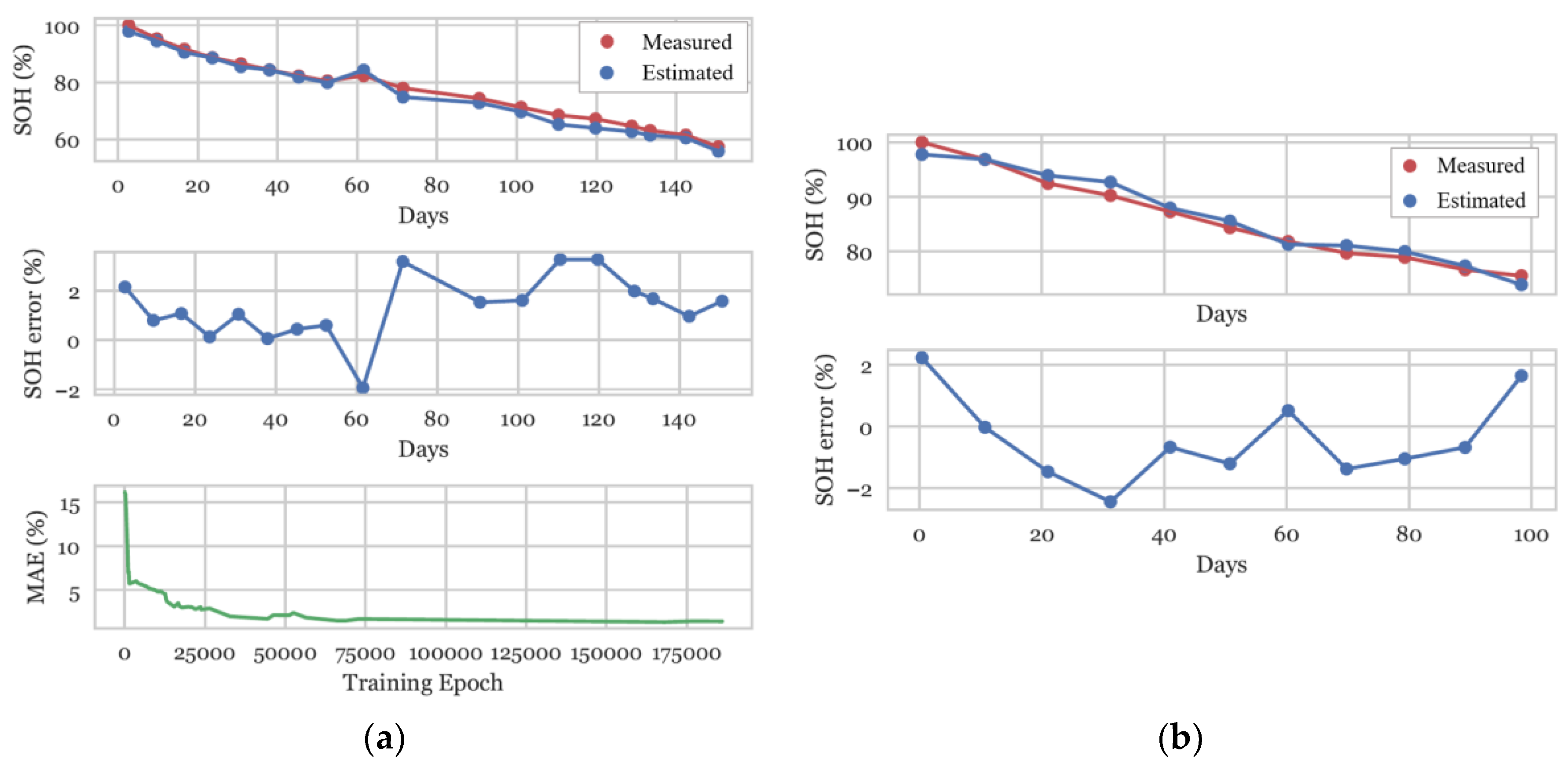
4.1. State-of-Health Estimation Using Fixed Charge Profiles

Training was conducted on up to 26 of the aging datasets and validation was performed on 1 or 2 datasets, depending on the tests being performed. The validation datasets are never seen by the CNN during the training process. The time required to train the CNNs used to obtain the results in this subsection was 4–9 h, depending on their size and depth.

The CNN was first validated on two aging datasets in the NASA repository, referred to as dataset RW4, recorded at 25 °C, and RW23, recorded at 40 °C. This CNN is composed of 6 convolution layers and 2 fully connected layers (FC). The results, shown in Figure 4 and in

Table 2. SOH estimation accuracy of CNN for 25 °C and 40 °C RW aging datasets.

Validation Dataset	MAE (%)	STDDEV (%)	MAX (%)
Validation RW dataset (25 °C)	1.5	1.0	3.3
Validation RW dataset (40 °C)	1.2	0.7	2.4

L1&L2: 32@(32,1), L3–L6: 64@(32,1), FC1: 256 neurons.

, point to an MAE of 1.5% and 1.2% for the 25 °C and 40 °C, respectively. The network is trained for up to 175,000 epochs. Mean absolute error is calculated as follows,

$$MAE=\frac{100\%}{n}{\displaystyle \sum }_{i=1}^{n}abs\left(\frac{SO{H}_i^{*}-SO{H}_i}{SO{H}_i^{*}}\right)$$

(7)

where n is the total number of discrete datapoints being evaluated.

The CNN’s performance over additional test cases are shown in

Table 3. SOH estimation accuracy of CNN for different test cases.

Case Study	MAE (%)	STDDEV (%)	MAX (%)	Parameters (Millions)
Input: voltage 1	1.5	1.1	3.9	3.8
Input: voltage, current, temperature 1	1.0	0.6	2.2	3.8
No pooling 1	1.3	0.8	3.4	3.8
Pooling 1	1.0	0.6	2.2	3.8
Unaugmented training data 2	2.4	1.1	4.2	3.6
Augmented training data 2	1.2	1.1	3.6	3.6
Smallest CNN 3	1.9	1.6	6.1	0.1

¹ L1–L6: 64@(32,1), FC1: 256 neurons, ² L1&L2: 32@(32,1), L3–L6: 64@(32,1), FC1: 256 neurons, ³ L1&L2: 4@(4,1), FC1: 32 neurons.

, where the footnotes indicate the architecture of the network. For example, L1: 32@(32,1), indicates that the first layer is a convolutional layer having 32 filters with height 32 and width 1. In addition to the performance metrics, the number of parameters representing the networks used for each of the test cases is shown. For most of these tests, training was stopped at 100,000 epochs to maintain testing objectivity. The first of such tests evaluates the CNN’s accuracy for inputs which include solely voltage as compared to inputs which include battery current, voltage and temperature. The results show that the error when using only voltage as an input is satisfactory with an MAE and MAX of 1.5% and 3.9% respectively. However, the MAE and the MAX are reduced by 33% and 44%, respectively, when using all three input signals. Therefore, all three inputs are critical for minimizing estimation error.

As described in Equation (1) of Section 2, max pooling, $S\left(·\right)$, is performed after a convolutional layer to subsample the layer activations. Although this is a layer that is often used for other applications, its efficacy in SOH estimation applications was initially unknown. Therefore, to better understand this, a CNN with pooling layers was compared to a second CNN with no pooling layers. It was found that a CNN with no pooling offered an MAE of 1.3% however a CNN with pooling had an MAE of 1.0%. Therefore, pooling improves the accuracy of the CNN for SOH estimation by about 23%.

In the third test, we investigated if augmented training data described in section III, affects the estimation accuracy of the CNN. This was performed by training two identical CNNs with identical architectures over augmented and unaugmented datasets. Augmentation describes the injection of Gaussian random noise as well as offsets and gains into the training data, as described in section III. Using an unaugmented training dataset, an MAE and MAX of 2.4% and 4.2% was obtained, while when using an augmented training dataset, an MAE and MAX of 1.2% and 3.6% was obtained. Therefore, exposing the CNN to augmented training datasets offers good performance gains with a reduction in MAE and MAX of 50% and 14%, respectively.

In the final test case, the estimation performance was examined for a much smaller network since on-board applications often cannot allocate a large amount of computation time to the SOH algorithm. Therefore, a network with only two convolutional layers was used to estimate SOH. When trained with augmented training data, the MAE and MAX achieved by this small CNN over a validation dataset were 1.9% and 6.1%, respectively. Although this network had adequate performance, further tests were conducted to assess the impact of network depth on the CNN. In Figure 5, the accuracy of convolutional neural networks at estimating SOH is recorded, first, as a function of network depth (number of layers) and, second, as a function of the amount of training data used during the training process. Clearly, deeper networks achieve increased estimation accuracy since going from 1 convolutional layer to 6 reduced the MAE by more than 60%.

In Figure 5b, the estimation accuracy over a validation dataset examined as a function of the amount of training is reduced. However, the argument to use more than 13 or 21 datasets during training becomes hard to substantiate given the diminishing improvement in accuracy. Models trained on battery measurements generated in the lab can be very sensitive to measurement noise, offsets and gains typically present in real world scenarios. Therefore, we tested the robustness of the CNN by using data that was intentionally augmented. In Figure 6 and in

Table 4. Results showing effect of augmented versus unaugmented validation dataset.

Validation Data Augmentation	MAE (%)	STDDEV (%)	MAX (%)
No	1.4	0.9	3.2
Yes 1	1.7	1.3	4.0

Architecture; L1–L4: 32@(31,1), FC1: 64 neurons, ¹ Augmented by injection of noise, gains, and offsets.

, the results for SOH estimation for augmented validation data are shown. Specifically, normally distributed random noise with mean 0 and standard deviation of 1%, 1.5% and 5% was added to the voltage, current and temperature measurements, respectively. An offset of 5 mV, 50 mA and 2 C was added to the voltage, current and temperature measurements, respectively. A gain of 2% was only applied to the current measurements. The CNN showed good robustness since performance over the augmented validation dataset resulted in a slightly higher MAE of 1.7%.

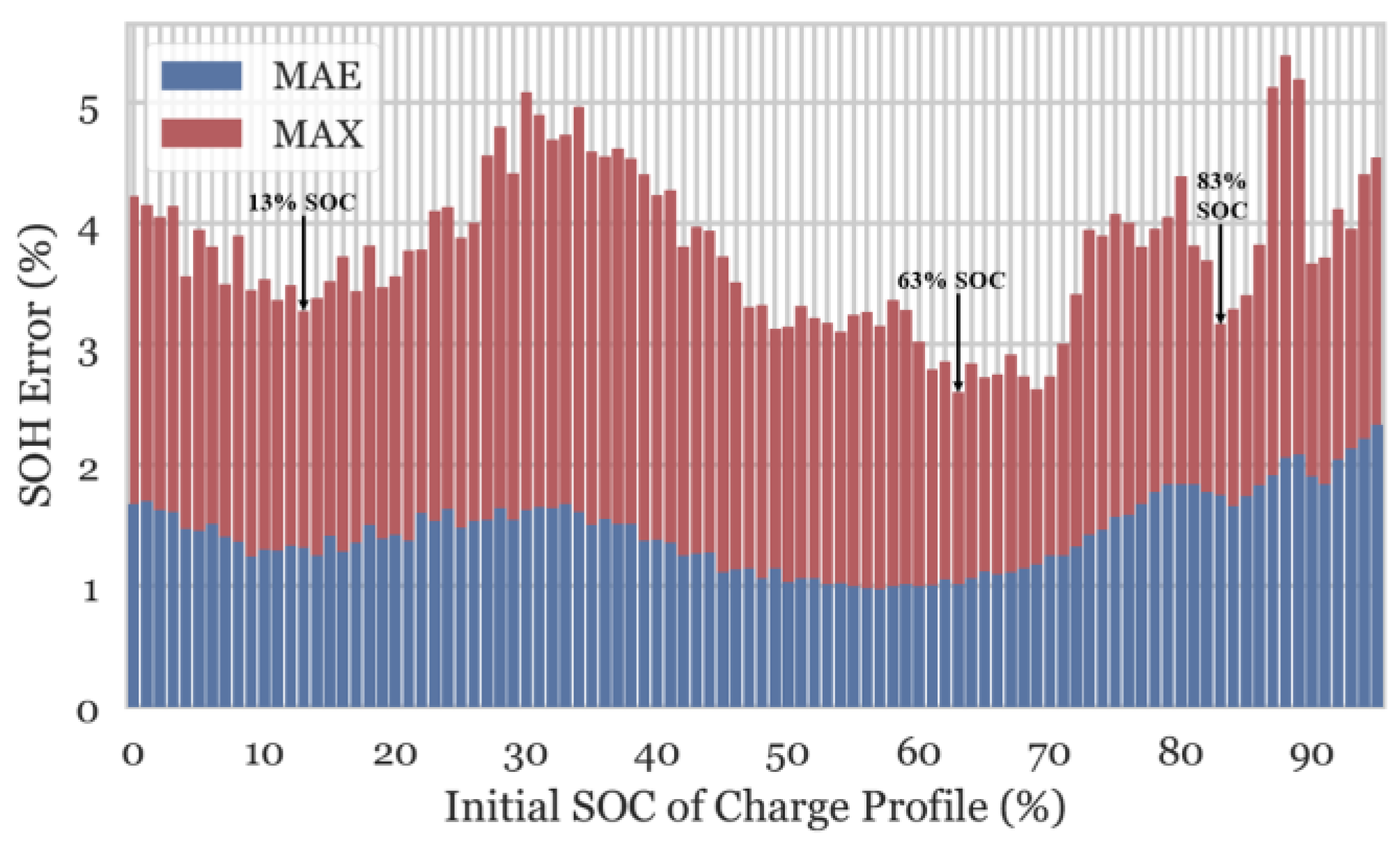
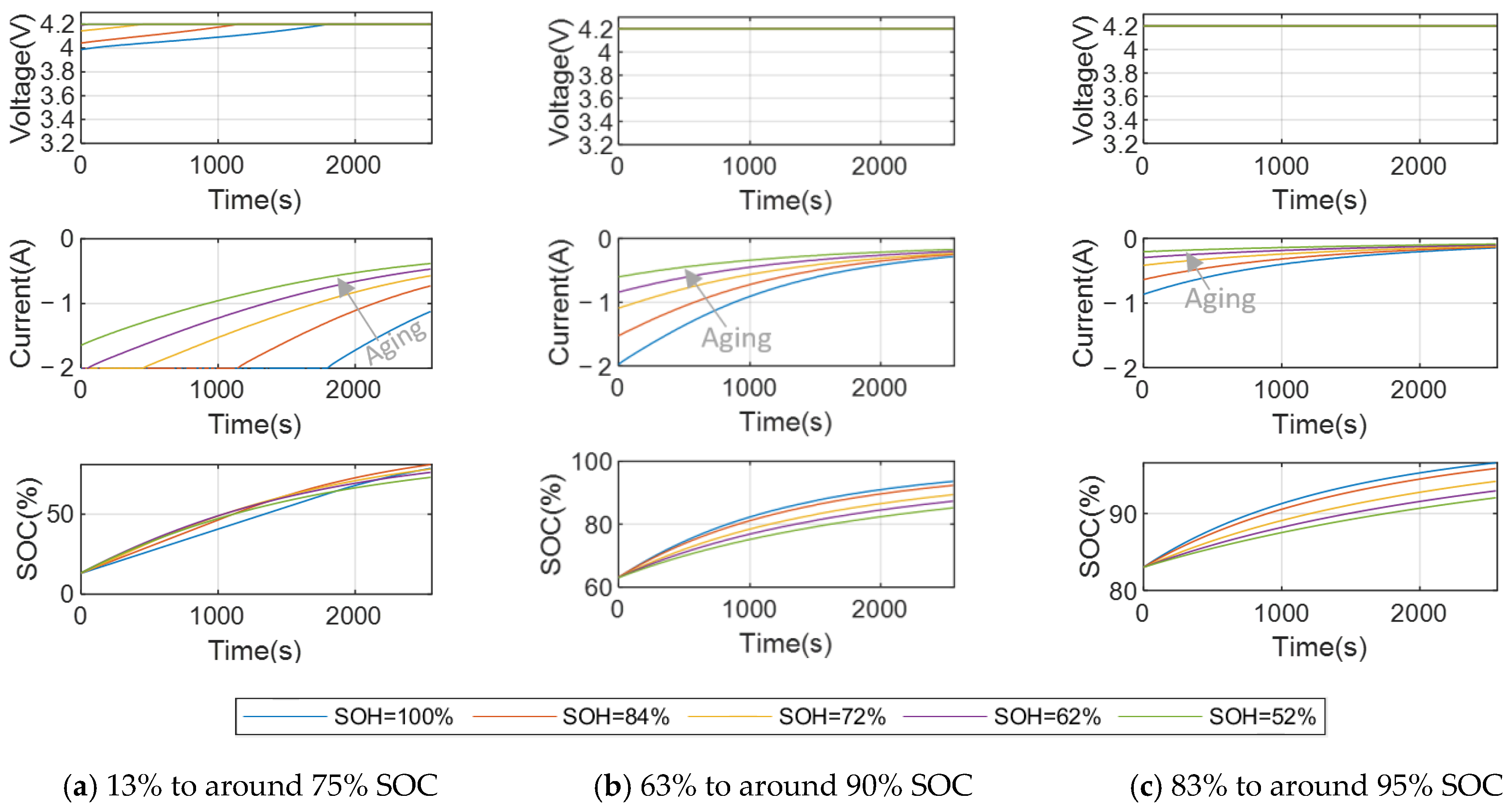
4.2. State-of-Health Estimation Using Partial Charge Profiles

Although the CNN achieved great performance in the previous subsection, the charge profiles used were fixed, such that the SOC ranged between 0% and about 60%. As described above, batteries are typically never fully discharged down to SOC = 0%. Therefore, to increase the practicality of this method, the CNN was trained over partial charge curves. However, differences between charge curves having different SOC ranges around the same SOH value can be subtle. Therefore, it becomes necessary to include something other than voltage, current and temperature as an input so that these subtle differences can be recognized by the CNN. Hence, SOC, which is assumed to be continuously monitored by an electric vehicle, for example, is included as an input to the CNN. The reference profiles ranging from SOC = 0% to SOC = 100% are typically longer than 1000 time steps, making it possible to select many different 256-length chunks to train on. Since the profiles were sampled once every 10 s, this meant that the length of each partial reference profile was about 43 min. It is important to note that in all the results of this subsection, all the stated ranges of the partial profiles were ranges of the new battery cell before it had aged. Although subsequent aged partial reference profiles started at the same SOC, they ended at a slightly lower state of charge. This can also be observed from the plots in Figure 7b and Figure 8b.

In Figure 7 and Figure 8, the SOH was estimated by the CNN using partial charge curves. In Figure 7, the SOC range of 30% to about 85% was used while in Figure 8 an SOC range of 60% to about 92% was utilized.

Table 5. SOH estimation error for different input SOC ranges. The stated ranges are for the battery when it was new.

SOC Range	MAE (%)	STDDEV (%)	MAX (%)
25 to 84%	1.6	1.1	3.6
40 to 89%	1.6	1.0	3.5
60 to 92%	0.8	0.7	2.7
85 to 97%	1.6	0.9	3.5

Architecture; L1 & L2: 64@(31,1), L3 & L4: 64@(16,1).

shows further results from other partial charge profiles having different SOC ranges. The SOC in these validation datasets was assumed to have a mean error of under 4% to simulate a real-world scenario. Although not overwhelmingly obvious, the results show that the larger SOC ranges generally resulted in better SOH estimation results. This is most likely attributed to the longer ranges of data which reveal more of the battery’s aging signature. However, the smaller SOC range of 85% to 97% achieved an MAE and a MAX of 1.6% and 3.5% which was nevertheless still good performance.

We performed SOH estimation with partial charge curves that sweep initial SOC from 0% to as high as 96% and the results are shown in Figure 9. The charge profiles begin at different SOC values, however, as mentioned above, they all have the same length of time of about 43 min. Interestingly, charge profiles beginning between an SOC of 5% and 20% and between an SOC of 50% and 70% had the lowest MAE and MAX error values. Those starting between an SOC of 30% and 40% had the highest. This can be attributed to the fact that the rate of change of the voltage is typically lower at an SOC of 30% to 40% and therefore this region has relatively fewer distinctive ageing features. Nevertheless, as can be observed from Figure 9, any 43 min window of data collected during a charge event, regardless of the initial SOC, can be used to achieve competitive SOH estimation accuracy.

For the results in Figure 9, there are 95 trained CNNs, one for each value of starting SOC. While this allows the SOH to be estimated with charge data starting at any SOC value, storing the parameters for all 95 CNNs would require an excessive amount of memory in a real-time application. The following design approach is therefore recommended: (1) Train CNNs with a wide range of starting SOC values, as shown in Figure 9; (2) Select the most accurate CNN in several different SOC ranges; (3) Implement the selected CNNs in the real time processor and update SOH whenever a charge with data in the corresponding SOC range is performed. As an example, three CNNs are marked in Figure 9 which are the most accurate in the nearby SOC range, those starting at 13% SOC, 63% SOC, and 83% SOC. Example charging data for these different SOC ranges is plotted in Figure 10 below, showing that as the battery aged, the current response during charging changed significantly, providing an excellent indicator of the SOH. In the real-time application, SOH would then be updated whenever a charge was performed that covered the 13 to 75%, 63 to 90%, or 83 to 95% SOC range. This methodology allows for more regular and accurate updating of the SOH estimate without requiring an excessive amount of memory for CNN parameters.

5. Conclusions

This paper introduced a deep learning technique for state-of-health estimation. Specifically, convolutional neural networks were used to extract ageing signatures from reference charge profiles and, in turn, estimate SOH. Time domain voltage, current, and temperature measurements were used as inputs to the CNN, and accuracy was found to be improved when data pooling was used and when the data was augmented with some noise and error to make it more representative of data from a real-world system. The use of more convolutional layers, up to six, was shown to reduce error. Little benefit was found for increasing the number of cells in the training dataset beyond 13, giving insight into how much battery testing is necessary to create an accurate machine learning-based SOH estimation algorithm. It was also demonstrated that by training the CNN with data at two different temperatures, the network accurately estimates SOH for charges at both temperature values. For applications with a wide temperature range, it is therefore recommended to train the network with data covering the whole span of operating temperatures. Importantly, it was shown that the CNN can accurately estimate SOH even when data is only available for a partial charge. A very wide range of partial charge cases were investigated, starting anywhere between 0 and 95% SOC, and ending between around 60 and 100% SOC, and MAE was no higher than 2.3% for these cases. A design approach is recommended where multiple CNNs are implemented in the real application, each trained for a different SOC range.

While other papers have utilized CNNs to estimate SOH from impedance spectroscopy data or combined CNNs with additional algorithms or methods for creating new features from the data, this work has shown that with proper CNN sizing and structure, sufficient data, and augmentation of the data through the addition of noise and error, a very low error of around 1% MAE or less can be achieved. The presented methodology is, overall, less complex than some of the prior art while still achieving good performance, making it a promising candidate for many applications.

References

1. Emadi, A. Advanced Electric Drive Vehicles; CRC Press: New York, NY, USA, 2015. [Google Scholar]
2. Rezvanizaniani, S.M.; Liu, Z.; Chen, Y.; Lee, J. Review and recent advances in battery health monitoring and prognostics technologies for electric vehicle (EV) safety and mobility. J. Power Sources 2014, 256, 110–124. [Google Scholar] [CrossRef]
3. Chen, Z.; Mi, C.; Fu, Y.; Xu, J.; Gong, X. Online battery state of health estimation based on Genetic Algorithm for electric and hybrid vehicle applications. J. Power Sources 2013, 240, 184–192. [Google Scholar] [CrossRef]
4. Yang, R.; Xiong, R.; He, H.; Mu, H.; Wang, C. A novel method on estimating the degradation and state of charge of lithium-ion batteries used for electrical vehicles. Appl. Energy 2017, 207, 336–345. [Google Scholar] [CrossRef]
5. Ouyang, M.; Chu, Z.; Lu, L.; Li, J.; Han, X.; Feng, X.; Liu, G. Low temperature aging mechanism identification and lithium deposition in a large format lithium iron phosphate battery for different charge profiles. J. Power Sources 2015, 286, 309–320. [Google Scholar] [CrossRef]
6. Ma, Z.; Wang, Z.; Xiong, R.; Jiang, J. A mechanism identification model based state-of-health diagnosis of lithium-ion batteries for energy storage applications. J. Clean. Prod. 2018, 193, 379–390. [Google Scholar] [CrossRef]
7. Vidal, C.; Malysz, P.; Kollmeyer, P.; Emadi, A. Machine Learning Applied to Electrified Vehicle Battery State of Charge and State of Health Estimation: State-of-the-Art. IEEE Access 2020, 8, 52796–52814. [Google Scholar] [CrossRef]
8. Sui, X.; He, S.; Vilsen, S.B.; Meng, J.; Teodorescu, R.; Stroe, D.-I. A review of non-probabilistic machine learning-based state of health estimation techniques for Lithium-ion battery. Appl. Energy 2021, 300, 117346. [Google Scholar] [CrossRef]
9. Severson, K.A.; Attia, P.M.; Jin, N.; Perkins, N.; Jiang, B.; Yang, Z.; Chen, M.H.; Aykol, M.; Herring, P.K.; Fraggedakis, D.; et al. Data-driven prediction of battery cycle life before capacity degradation. Nat. Energy 2019, 4, 383–391. [Google Scholar] [CrossRef] [Green Version]
10. Rastegarpanah, A.; Hathaway, J.; Stolkin, R. Rapid Model-Free State of Health Estimation for End-of-First-Life Electric Vehicle Batteries Using Impedance Spectroscopy. Energies 2021, 14, 2597. [Google Scholar] [CrossRef]
11. Shen, S.; Sadoughi, M.; Chen, X.; Hong, M.; Hu, C. A deep learning method for online capacity estimation of lithium-ion batteries. J. Energy Storage 2019, 25, 100817. [Google Scholar] [CrossRef]
12. Fan, Y.; Xiao, F.; Li, C.; Yang, G.; Tang, X. A novel deep learning framework for state of health estimation of lithium-ion battery. J. Energy Storage 2020, 32, 101741. [Google Scholar] [CrossRef]
13. Yang, N.; Song, Z.; Hofmann, H.; Sun, J. Robust State of Health estimation of lithium-ion batteries using convolutional neural network and random forest. J. Energy Storage 2022, 48, 103857. [Google Scholar] [CrossRef]
14. Jo, S.; Jung, S.; Roh, T. Battery State-of-Health Estimation Using Machine Learning and Preprocessing with Relative State-of-Charge. Energies 2021, 14, 7206. [Google Scholar] [CrossRef]
15. Klass, V.; Behm, M.; Lindbergh, G. A support vector machine-based state-of-health estimation method for lithium-ion batteries under electric vehicle operation. J. Power Sources 2014, 270, 262–272. [Google Scholar] [CrossRef]
16. Eddahech, A.; Briat, O.; Bertrand, N.; Deletage, J.-Y.; Vinassa, J.-M. Behavior and state-of-health monitoring of li-ion batteries using impedance spectroscopy and recurrent neural networks. Int. J. Electr. Power Energy Syst. 2012, 42, 487–494. [Google Scholar] [CrossRef]
17. Feng, X.; Li, J.; Ouyang, M.; Lu, L.; Li, J.; He, X. Using probability density function to evaluate the state of health of lithium-ion batteries. J. Power Sources 2013, 232, 209–218. [Google Scholar] [CrossRef]
18. Weng, C.; Cui, Y.; Sun, J.; Peng, H. On-board state of health monitoring of lithium-ion batteries using incremental capacity analysis with support vector regression. J. Power Sources 2013, 235, 36–44. [Google Scholar] [CrossRef]
19. Wang, Z.; Ma, J.; Zhang, L. State-of-Health Estimation for Lithium-Ion Batteries Based on the Multi-Island Genetic Algorithm and the Gaussian Process Regression. IEEE Access 2017, 5, 21286–21295. [Google Scholar] [CrossRef]
20. Guo, Z.; Qiu, X.; Hou, G.; Liaw, B.Y.; Zhang, C. State of health estimation for lithium ion batteries based on charging curves. J. Power Sources 2014, 249, 457–462. [Google Scholar] [CrossRef]
21. Bole, B.; Kulkarni, C.S.; Daigle, M. Randomized Battery Usage Dataset; NASA Ames Prognostics Data Repository, Tech. Rep.; Ames Research Center: Mountain View, CA, USA, 2014.
22. Deng, L. Deep Learning: Methods and Applications. Found. Trends Signal Processing 2014, 7, 197–387. [Google Scholar] [CrossRef] [Green Version]
23. Goodfellow, I.; Bengio, Y.; Courville, A. Deep Learning; MIT Press: Cambridge, MA, USA, 2016; Available online: http://www.deeplearningbook.org (accessed on 2 February 2022).
24. LeCun, Y.; Bengio, Y.; Hinton, G. Deep learning. Nature 2015, 521, 436–444. [Google Scholar] [CrossRef]
25. Krizhevsky, A.; Sutskever, I.; Hinton, G.E. ImageNet Classification with Deep Convolutional Neural Networks. Adv. Neural Inf. Processing Syst. 2012, 25, 1–9. [Google Scholar] [CrossRef]
26. Ciresan, D.; Meier, U.; Masci, J.; Schmidhuber, J. Multi-column deep neural network for traffic sign classification. Neural Netw. 2012, 32, 333–338. [Google Scholar] [CrossRef] [Green Version]
27. Hinton, G.; Deng, L.; Yu, D.; Dahl, G.E.; Mohamed, A.-R.; Jaitly, N.; Senior, A.; Vanhoucke, V.; Nguyen, P.; Sainath, T.N.; et al. Deep Neural Networks for Acoustic Modeling in Speech Recognition: The Shared Views of Four Research Groups. IEEE Signal Process. Mag. 2012, 29, 82–97. [Google Scholar] [CrossRef]
28. Ciregan, D.; Meier, U.; Schmidhuber, J. Multi-column deep neural networks for image classification. In Proceedings of the 2012 IEEE Conference on Computer Vision and Pattern Recognition, Providence, RI, USA, 16–21 June 2012; pp. 3642–3649. [Google Scholar]
29. He, K.; Zhang, X.; Ren, S.; Sun, J. Deep Residual Learning for Image Recognition. In Proceedings of the 2016 IEEE Conference on Computer Vision and Pattern Recognition (CVPR), Las Vegas, NV, USA, 27–30 June 2016; pp. 770–778. [Google Scholar]
30. Ma, J.; Sheridan, R.P.; Liaw, A.; Dahl, G.E.; Svetnik, V. Deep neural nets as a method for quantitative structureactivity relationships. J. Chem. Inf. Modeling 2015, 55, 263–274. [Google Scholar] [CrossRef]
31. Leung, M.K.K.; Xiong, H.Y.; Lee, L.J.; Frey, B.J. Deep learning of the tissue-regulated splicing code. Bioinformatics 2014, 30, i121–i129. [Google Scholar] [CrossRef] [Green Version]
32. Xiong, H.Y.; Alipanahi, B.; Lee, L.J.; Bretschneider, H.; Merico, D.; Yuen, R.K.C.; Hua, Y.; Gueroussov, S.; Najafabadi, H.S.; Hughes, T.R.; et al. The human splicing code reveals new insights into the genetic determinants of disease. Science 2015, 347, 1254806. [Google Scholar] [CrossRef] [Green Version]
33. Wang, D.; Khosla, A.; Gargeya, R.; Irshad, H.; Beck, A.H. Deep Learning for Identifying Metastatic Breast Cancer. arXiv, 2016; arXiv:1606.05718. [Google Scholar]
34. Kingma, D.P.; Ba, J. Adam: A Method for Stochastic Optimization. CoRR, vol. abs/1412.6980. 2014. Available online: http://arxiv.org/abs/1412.6980 (accessed on 2 February 2022).
35. Analog Devices. LTC6813-1. Analog Devices, Inc.: Wilmington, MA, USA, 2018. Revision: A. Available online: https://www.analog.com/media/en/technical-documentation/datasheets/LTC6813-1.pdf (accessed on 2 February 2022).
36. LEM. Automotive Current Transducer Fluxgate Technology CAB 500-C/SP5, Version: 0; LEM Europe GmbH: Plan-les-Ouates, Switzerland, 2018.
37. Murata. Thermistor NTC 10K; Murata Manufacturing Co., Ltd.: Kyoto, Japan, 2018. [Google Scholar]
38. An, G. The Effects of Adding Noise During Backpropagation Training on a Generalization Performance. Neural Comput. 1996, 8, 643–674. [Google Scholar] [CrossRef]
39. Srivastava, N.; Hinton, G.E.; Krizhevsky, A.; Sutskever, I.; Salakhutdinov, R. Dropout: A simple way to prevent neural networks from overfitting. J. Mach. Learn. Res. 2014, 15, 1929–1958. [Google Scholar]
Figure 1. Architecture of a convolutional neural network (CNN) where each layer is composed of a convolution and pooling component and with the last two layers being fully connected. The input data is given by Ψ ( ξ ) N × M where N = 256 and M = 3 since Ψ ( ξ ) = [ I ( ξ ) ; V ( ξ ) ; T ( ξ ) ] where I, V and T represent the current, voltage and temperature of the charge curve. The output of the CNN is the estimated SOH.
Energies 15 01185 g001
Figure 2. (a) CC segment of charge profile of a Li-ion cell throughout randomized usage aging process; color spectrum of profiles indicate SOH. (b) Recorded capacity-based SOH for each of the charge profiles in (a).
Energies 15 01185 g002
Figure 3. Flowchart describing data preprocessing, data augmentation and model training steps. Each of the datasets are constructed by extracting the reference charge profiles from the raw data. After preprocessing, the 28 datasets are split into train and testing datasets. The train set is then augmented as described in Section 3 before training begins. Please refer to text for more details.
Energies 15 01185 g003
Figure 4. (a) From top to bottom, CNN estimation accuracy, estimation error over the 25 °C validation dataset and the mean absolute error as a function of training epochs. (b) Estimation accuracy and estimation error over 40 °C validation dataset.
Energies 15 01185 g004
Figure 5. (a) Estimation accuracy over validation data versus number of layers in CNN. (b) Estimation accuracy measured during validation versus number of training datasets. All tests were performed over validation datasets recorded at 25 °C.
Energies 15 01185 g005
Figure 6. (a) Augmented and unaugmented voltage, current and temperature signals of validation dataset. (b) Estimation accuracy and error for augmented and unaugmented battery validation data. Please see Table 4 for detailed results.
Energies 15 01185 g006
Figure 7. (a) CNN SOH estimation and error for partial charge curve input beginning at 30% SOC and ending at about 85% SOC. (b) Partial charge profiles beginning at 30% SOC and ending at about 85% SOC.
Energies 15 01185 g007
Figure 8. (a) CNN SOH estimation and error for partial charge curve input beginning at 60% SOC and ending at about 92% SOC. (b) Partial charge profiles beginning at 60% SOC and ending at about 92% SOC.
Energies 15 01185 g008
Figure 9. MAE and MAX values of SOH estimation performed over charge profiles beginning at various SOC values. The partial charge profiles are obtained from the NASA prognostics repository and are about 43 min long. The stated ranges of the partial profiles are ranges of the new battery cell before it has aged.
Energies 15 01185 g009
Figure 10. Examples of voltage, current, and SOC time domain charging measurements used for training SOH algorithm. Each set of partial SOC charge data is 2560 s long, the input data length for the CNN.
Energies 15 01185 g010