Self-Powered Wireless Sensor Matrix for Air Pollution Detection with a Neural Predictor

Abstract

Predicting the status of particulate air pollution is extremely important in terms of preventing possible vascular and lung diseases, improving people’s quality of life and, of course, actively counteracting pollution magnification. Hence, there is great interest in developing methods for pollution prediction. In recent years, the importance of methods based on classical and more advanced neural networks is increasing. However, it is not so simple to determine a good and universal method due to the complexity and multiplicity of measurement data. This paper presents an approach based on Deep Learning networks, which does not use Bayesian sub-predictors. These sub-predictors are used to marginalize the importance of some data part from multisensory platforms. In other words—to filter out noise and mismeasurements before the actual processing with neural networks. The presented results shows the applied data feature extraction method, which is embedded in the proposed algorithm, allows for such feature clustering. It allows for more effective prediction of future air pollution levels (accuracy—92.13%). The prediction results shows that, besides using standard measurements of temperature, humidity, wind parameters and illumination, it is possible to improve the performance of the predictor by including the measurement of traffic noise (Accuracy—94.61%).

1. Introduction

The subject of air quality study and prediction is a very important research area [1,2,3]. As reported by the authors [4], air pollution prediction methods can be divided into statistical, numerical, neural network and hybrid models. One of the most common problems in the analysis of multisensory systems is the presence of noise and faulty measurements in the learning dataset. To counteract this state, data marginalization is performed using Bayesian sub-predictors. Bayesian sub-predictors also allow for extrapolation of missing data. However, their disadvantage is that they increase the complexity of the algorithm architecture and increase the computational cost. The novelty of the proposed algorithm is that it proposes a built-in algorithm for clustering features from non-image data in such a way that there is a formation of an image of the extracted features, which groups these features and thus increases the effectiveness of the neural predictor itself. This paper presents experimental results for a neural prediction system for particulate air pollution. The input data are data acquired using a designed self-organizing wireless sensor matrix (WSM). The decision system was focused on evaluating the influence of atmospheric conditions and historical particulate matter on smog occurrence. The effects of temperature, humidity, wind speed and wind direction, and historical particulate matter measurement data on PM10, PM2.5, PM1 were analyzed. The architecture of a single measurement platform in terms of Energy Harvesting (EH) system, energy storage system and sensor systems were also presented. The architecture of communication between the nodes of the WSM network is also presented. The novelty of the paper is also the use of Deep Learning algorithm, in addition to classical Neural Network architectures, to extract the features of the raw tabular data vector. This approach allows the attainment of better results for the prediction of future air pollution. The platform presented in this paper is a self-developed embedded system, whose various versions are present in technology. However, the most important aspect of this work is the non-Bayesian predictor itself in Deep Learning networks. This is because data marginalization can however lead to the removal of parts of the data that are meaningful. Of course, various research centers are working on improving this mechanism, but this work presents a different approach. This approach is based on not using marginalization, but direct inference from raw tabular data, transformed to image form using a special feature extractor. This approach has improved the quality of prediction and in the future can be applied for other branches of technology than air pollution prediction, such as predictive maintenance, medical, economic and social sciences.

2. Study Area

Wireless sensors are of high interest in many academic and business research centers [5,6,7]. The biggest advantage of this type of sensor is that no or limited maintenance is required. Basically, the need to supply power and communication cables to such a device is eliminated. Most often, in addition to the energy source such a system is equipped with energy storage in the form of batteries and a wireless communication system [8,9]. The advantage of such systems makes them applicable in a very wide range of applications—from monitoring environmental variables to measurements in hard-to-reach places of machines, devices and systems. The basic requirement for such systems is resistance to external factors and possibly long maintenance-free operation. This time can be increased by three strategies: lowering the power demand of the system, using more powerful energy storage or by using Energy Harvesting (EH). It is best to look for a combination of all three; however, only EH can extend the maintenance-free time of the platform in a non-linear way and even beyond the expected lifetime. Many research centers are working on self-powered sensing circuits for integrating wireless sensing, energy harvesting, power management and energy storage, and data processing [10,11].Research also includes the development of antennas [12], energy harvesting from unusual sources such as hydraulic vibrations [13] or even nanotribological sources [14]. Interestingly, according to [15], the use of multi-scale sensors and biosensors in the multisensor platform could significantly improve the quality of detection in medicine as well, more effectively identifying possible SARS-CoV-2 virus infections.

A variety of methods are used in EH to generate energy. One of the most commonly used is the use of photovoltaic panels. The analysis presented in [16] leads to relationships determining what initial charge and duty cycle power consumption values are necessary to obtain a self-sustaining system at a given average sunlight level. The authors formulate schemes for adapting duty cycle and other software platforms. The disadvantage of a photovoltaic-based solution is, of course, the need for access to natural light sources, i.e., limitations to outdoor applications. Nevertheless, an interesting solution to this problem is the use of panels based on perovskite [17]. The proposed solution can extract energy from artificial light quite efficiently [18]. Another family of EH solutions is the extraction of electricity from thermal energy [19,20]. This method uses direct conversion of temperature difference into electric voltage according to the Seebeck effect occurring at the interface between two semiconductors at different temperatures. According to [21], this is one of the best methods to obtain microenergy to power sensor systems using residual heat. One possible variation of this method is pyroelectrics [22]. Here, dielectric materials are used for which the amount of charge released depends on the polarization intensity. Among other EH methods, one can certainly list: mechanical [23,24], electromagnetic [25,26] or hybrid [27] methods. A whole range of interesting solutions related to self-powered sensors are solutions based on nanopolymers and other smart materials [28,29,30]. In this case, advances in modern materials science allow for unheard of minimization of EH systems. It is also possible to achieve high efficiency and take advantage of the increasingly lower differences between energy potentials in power generation. The system presented in this paper can use each of the above-mentioned forms of EH separately. The system architecture also allows for hybrid incorporation of EH sources. The results presented here include a photovoltaic panel as a source. An essential component of air pollution is particulate matter (PM). They are formed mostly as a result of combustion reactions, and they are small particles composed of various substances and chemical compounds. According to the Polish definition, dusts are solid particles of various sizes and origin, suspended in a gas for a certain period of time. Aerosol, on the other hand, is a suspension of solid, liquid, or solid and liquid particles in a gas phase with a negligible rate of drop. On the other hand, international agencies focused on environmental protection, i.e., the WHO, Geneva (World Health Organization), US EPA, Washington (United States Environmental Protection Agency), EEA, Copenhagen (European Environment Agency) provide a definition of the term particulate matter, or PM (Particulate Matter), as the dispersed phase of aerosol and define it as a mixture of solid and liquid particles suspended in the air. Particulate matter is classified by grain size, and three types of particulate matter are distinguished:

• PM10, with particles of no more than 10 $\mathsf{\mu }$m;
• PM2.5, with particles not exceeding 2.5 $\mathsf{\mu }$m;
• PM1, with particles not exceeding 1 $\mathsf{\mu }$m.

Types of dust, resulting from the above division, are characterized by different sources of formation, and thus properties and chemical composition. Due to these differences, they affect health differently and their removal requires different methods. As the size of dusts decreases, their danger increases due to the difficulty of filtration or subsequent removal. This mainly concerns the possibility of penetration into the breathing systems of humans and animals. In the scope of work, it was necessary to determine boundary conditions, which were based on standards of concentration of particulate matter. Further conditions were determined depending on the type of dust. PM10 dust contains carcinogenic heavy metals such as benzopyrenes, furans and dioxins. It is dangerous not only because of its contribution to breathing diseases, but also its high concentration increases the risk of heart attack and stroke.

• The permissible level of 24 h average concentration is 50 $\mathsf{\mu }$g/m${}^3$, not exceeing more than 35 days a year;
• The limit for annual average concentration is 40 $\mathsf{\mu }$g/m${}^3$;
• The information level for 24 h concentration is 200 $\mathsf{\mu }$g/m${}^3$;
• The alert level for 24 h concentration is 300 $\mathsf{\mu }$g/m${}^3$.

PM2.5 fine particulate matter contains secondary aerosols and combustion particles. It is particularly dangerous to human health because it can penetrate the pulmonary alveoli and thus cause a number of dangerous and even fatal diseases. It remains in the air for up to several weeks and cannot be removed by sedimentation or precipitation. PM1 is the most dangerous of the particulates tested. Their fine particles penetrate through the lungs directly into the bloodstream and spread to the human organs. This causes problems with the circulatory, respiratory and nervous systems. There are many methods for determining particulate matter in the air. The gravimetric method, otherwise known as the reference method, is recognized worldwide as the most precise [31]. Its disadvantage is the long waiting time for the result, which is three weeks. It involves a daily replacement of the filter into which atmospheric air is drawn. Each filter is weighed and has its own unique identification number before being installed. After two weeks, the filters are collected and transported to a laboratory where they are weighed and conditioned again. The concentration result is given based on the weight difference related to the airflow volume of the filter. Another method that can be used to measure dust concentration is the laser light scattering method, or laser diffraction. It is characterized by a low cost of determination and simple dust collection, although a major disadvantage of this method is the increase in measurement uncertainty for other than spherical dust grains [32]. It is based on the use of the ultrasonic method to guide the dust from the measuring strainers to the depressing medium. Then the actual determination occurs on a laser granulometer. The phenomenon of optical diffraction of monochromatic light, which occurs at the boundary between an impervious medium and a transmissive medium, i.e., dust particles and a depressing liquid that forms an optical medium, is used to determine the particulate amount.

Indirect methods are a very interesting solution, and are mostly based on image analysis and using Deep Learning (DL) neural networks [33]. In this case, two datasets are applied to the model. The learning data contain synthetic images with prepared PM concentration labels. The second set contains actual images and numerical weather data from a weather station. The authors [33] present a parameter optimization model to distinguish fog from smog and improve the accuracy of smog occurrence prediction. Other neural methods for image analysis are also used. One of the more commonly used is SVM [34,35]. The proposed SVM method is well suited for classification and pattern recognition tasks. This method is used in remote sensing of air pollution due to its characteristics, which makes intensive use of the data itself and is not limited by the distributional assumptions of the data. The class of supervised learning algorithms used in air pollution detection can also include Classification and Regression Trees (CART) [36] and K-Nearest Neighbors (KNN) [37,38]. However, the biggest disadvantage of supervised algorithms is the need to prepare and label large datasets. Additionally, they can generate false positives or false negatives when the environment changes.

The use of Unsupervised Learning Networks can solve many of the mentioned problems. Most importantly, networks with architectures such as Multilayer Perceptron (MLP) [39], Convolutional Neural Networks (CNN) [40], and Recurrent Neural Networks (RNN) [41], allows for the direct use of raw data. It also eliminates the need for data labeling. This is because networks with these architectures have a feature extractor. With its help, it is possible to transform the raw data into an appropriate feature vector. Deep Learning Networks learn the hidden features of raw data by using the representation learning method. Hence, they can detect dependencies in the model that are hidden to the expert without being biased by incomplete knowledge about the system.

A very interesting model for studying the Air Quality Index based on The Hybrid EMD–SARIMA method is presented in [42]. In this model, a time series is decomposed into forecast parts using the seasonal auto regressive integrated moving average method, followed by forecast re-composition. In air pollution prediction, Machine Learning can also be used to create spatial maps of elevated PM levels. Such an approach has been used in [43], where maps of PM10 concentrations were successfully produced from landform and building data, soil data, and temperature and wind data. Deep Learning predictors based on gated recurrent unit networks for Internet of Things sensors data have been presented in [44]. In this case, prediction accuracy was improved by combining partial forecasts using sub-predictors. The class of methods using Machine Learning also includes the one presented in [45]. This paper presents a prediction estimation method using the series causality entropy method. The Bayesian approach in MLP networks presented by Jin et al. features high robustness to sensor noise. The Bayesian method is used here to obtain the weight distribution for the sub-predictor. The proposed causal entropy method allows efficient feature extraction from multi-sensor systems. The novelty presented by Jin et al. is a multistage Bayesian prediction system applied to reduce the dimensionality of feature selection to overcome data noise. This is because the effect of data noise affects the learning efficiency of MLP networks. In general, Bayesian networks determine continuous prior distributions for each bias and weight. This, however, results in difficult inference due to the huge parameter space of the [46]. However, the advantage of such networks is that they lead to improved system calibration, i.e., a more consistent expression of uncertainty. In such systems, the correctness of the classifier calibration is determined positively if the confidence of the prediction is equal to the misclassification rate. Such marginalization therefore improves the accuracy of the modern neural networks [47].

3. System Architecture

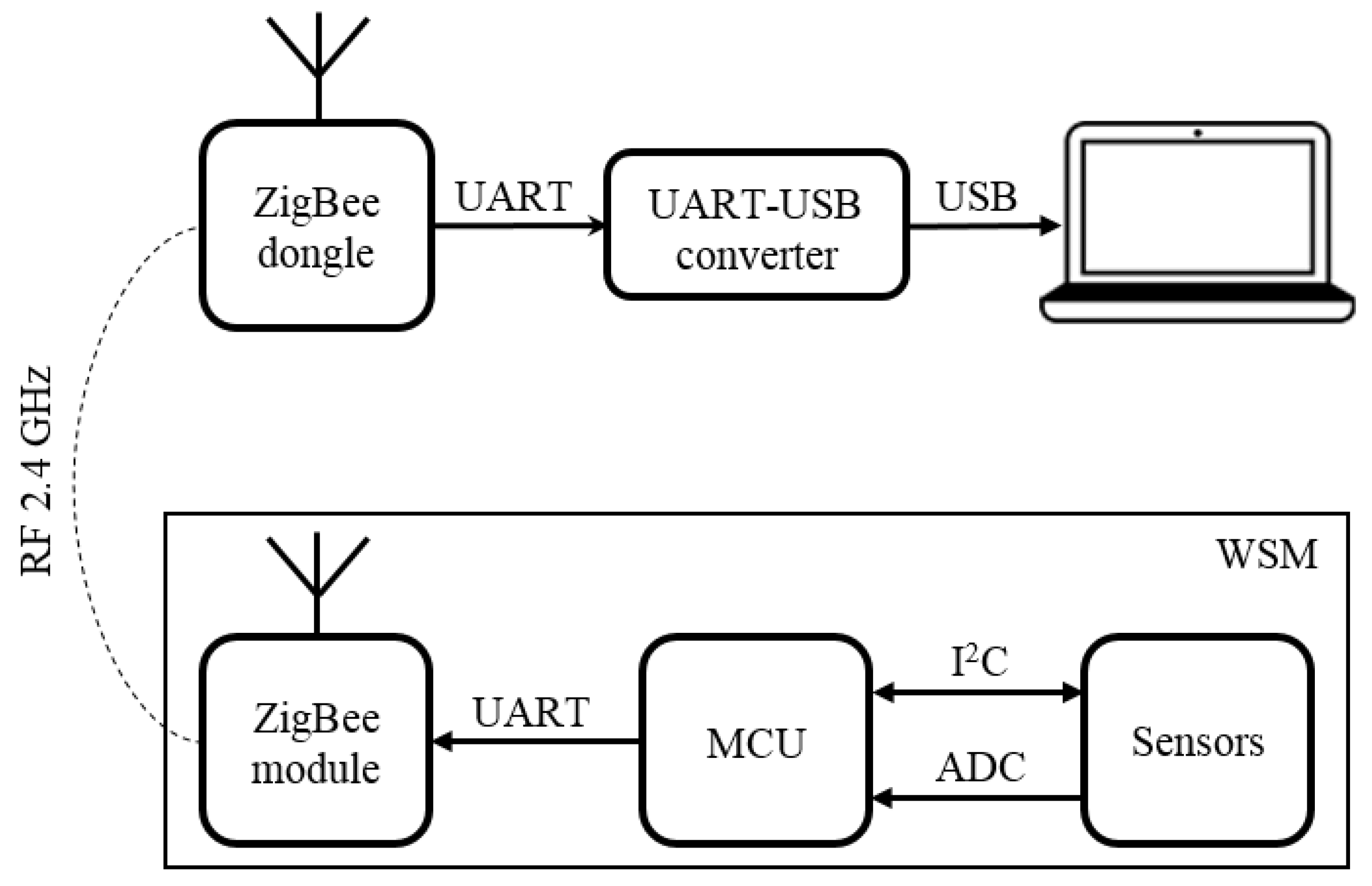
The system consists of 5 wireless platforms including 4 slave nodes and one master node. The research methodology is to distribute them at a distance of 50 m to collect information from an area of about 200 m${}^2$. The artificial neural network is designed to treat as input not only the information from the sensors of one platform, but from several at the same time, and on this basis to predict the future air pollution. The number of sensors can be expanded. 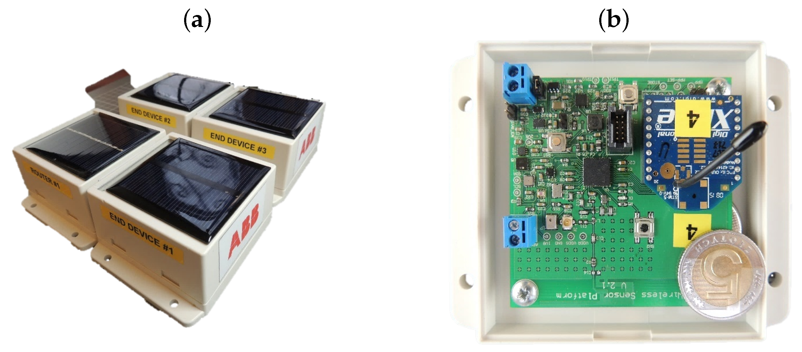A concept of the system was presented in Figure 1 in a graph form. The Figure 2, shows pictures of the final form of the executive part of the system, the WSM from inside and the ZigBee Dongle correspondingly.

The platform was equipped with 9 sensor systems. First, the illuminance sensors (TI OPT3001) was used. The next sensor was an atmospheric pressure sensor (Alps HSPPAD) and humidity and temperature sensors (Alps HSHCAL). The measurements of UV-A and UV-B radiation sensors (Alps HSUDDD) were also studied along with a wind speed and direction sensor. A PM1, 2.5 and 10 sensor type PMS3003 was also added. In addition, car traffic volume was found to be an important data for the neural prediction system, hence a MEMS microphone (STM MP34DT02) was also included.

3.1. Master Control Unit

The Master Control Unit (MCU) has a key role in managing the entire platform. It is primarily tasked with managing the Energy Harvesting circuits and the energy storage. The state machine of the platform is also implemented in the MCU. This means the MCU manages the platform states and ensures power demand reduction and system self-diagnostics. Another task of the MCU is to collect sensor data, preprocess it and encapsulate the data into a communication protocol. The last task is communication with other units and intelligent routing with other nodes in the network and eventually master node. The main Integrated Circuit (IC) that was applied to the device is CC2630 MCU manufactured by TI. It is a member of wireless CC26xx family targeting ZigBee and 6LoWPAN applications. The family of the ICs are cost-effective, ultralow power and 2.4 GHz radio frequency capable. Furthermore, it consists of an ultralow power Sensor Controller, which can be used for collecting analog and digital data autonomously while the rest of the system is in a sleep mode. That is why the MCU is an accurate choice for its ability to be powered by small coin cell batteries, energy harvesting, wireless communication applications. Essentially, the features of the design of the device are following:

• Main CPU: 48 MHz ARM Cortex M3, 128 KB flash memory, 20 KB SRAM;
• Peripherals: 8 × 12-bit ADC 200 ksample/s, I2C, UART, RTC, 31 GPIOs;
• Sensor Controller current consumption in active mode: 394 $\mathsf{\mu }$A;
• Overall current consumption: 2.94 mA in active mode, 1 $\mathsf{\mu }$A in standby (RTC running and RAM/CPU retention);
• Current consumption of the RF module:

  −

  Receiving: 5.9 mA;

  −

  Transmitting at 0 dBm output power (software programmable): 6.1 mA;

  −

  Transmitting at +5 dBm output power (software programmable): 9.1 mA;

• RF receiver sensitivity: −100 dBm;
• Supply voltage range: 1.8–3.8 V.

The MCU provides 4 software configurable power modes: active, idle, standby and shutdown. The active mode is the mode which provides full performance of the MCU but it come at a price for power consumption. In this mode, code is actively executed and all of the peripherals that are currently enabled provide normal operation. The system clock can be any available clock source. The mode is present for example during UART communication. Current consumption in this state is about 2.94 mA.

The idle mode is used when the CPU is not being unused; however, the MCU cannot go into deeper power-saving modes due to the fact that waking up from them consumes more time than is reserved for power-saving. All active peripherals can be clocked, but the System CPU core and memory are not clocked as well as code not being executed. Any interruption event will bring the processor back into active mode. Current consumption in this state is about 550 $\mathsf{\mu }$A.

In the standby mode, only the always-on domain (AON) is active. A pin, RTC or Sensor Controller interrupt event is required to bring the device back to active mode. The MCU peripherals do not need to be reconfigured when waking up again and the System CPU continues code execution from where it went into standby mode. All GPIOs are latched to the state just before entering standby mode. Current consumption in this state is about 1 $\mathsf{\mu }$A.

In the shutdown mode, the MCU is turned off entirely, including the AON domain and the Sensor Controller. All GPIOs are latched to the state just before entering standby mode. A pin interrupt defined as a wake from the shutdown wakes up the MCU and acts as a reset. The Sensor Controller is an autonomous processor that can control the peripherals, which are placed in the AUX domain, independently of the System CPU. Therefore, the System CPU does not have to wake up, for instance to perform an ADC sample or poll a digital sensor over I2C. The System CPU saves both current consumption and wake-up time that would otherwise be wasted. The Sensor Controller is placed in the AUX domain of the MCU. The AUX is a common description of all the analog and the digital modules in the AUX power domain such as the Sensor Controller, timers, time to digital converter, and others. The AUX power domain is located within the AON domain of the MCU. The Sensor Controller can conduct its own power and clock management of the AUX power domain, independently of the System CPU.

The enabling components essential for the MCU include a group of decoupling capacitors: C1–C4, C6, C8, C9 and C20, capacitors C5, C7, and an inductor L1 is required for properly work of the integrated DC/DC converter, electromagnetic coupling filter FL1 for GHz noise, pull-up resistor R1 for the reset pin, microswitch SW1 for resetting the MCU, custom pinout JTAG connector J1 and two quartz crystal oscillators: high frequency 24 MHz and low frequency 32,768 kHz. Generally, the high frequency oscillator is used in normal work of the MCU, whereas the low frequency oscillator is used in the device sleeping mode for RTC clocking. The MCU provides internal crystal load capacitance for high frequency oscillator in the range from 2 pF to 11 pF; thus, external capacitors are unnecessary. However, the low frequency oscillator are not provided with this feature, therefore 9 pF external capacitors were included.

The MCU was integrated with the 2.4 GHz radio module supporting ZigBee and 6LoWPAN networks. It supports two front end output options: differential and single-ended with internal or external bias. The front ends provide different values of sensitivity and output power. The target front end was selected as differential with internal bias, which features an −99 dBm sensitivity and +5 dBm output power. The application of the integrated radio is presented in Figure 3. The radio module was designed to work with PCB printed or chip antennas. The project application includes the “Inverted F” PCB printed antenna of which the layout is presented in Figure 4. The dimensions of the antenna are showed in the

Table 1. Inverted F PCB printed antenna dimensions.

Label	Value (mm)	Label	Value (mm)
H1	5.70	W2	0.46
H2	0.74	L1	25.58
H3	1.29	L2	16.40
H4	2.21	L3	2.18
H5	0.66	L4	4.80
H6	1.21	L5	1.00
H7	0.80	L6	1.00
H8	1.80	L7	3.20
H9	0.61	L8	0.45
W1	1.21

. This solution provides low cost, ultra-low power consumption and high performance of the radio module.

Some of the peripherals are embedded into the PCB. The LED D1 indicates the successful startup sequence of the device. Microswitch SW2 was used for debugging purposeas. An I2C sensor application, which consists of 4 sensors with decoupling capacitors and I2C’s bus pull-up resistors is presented in Figure 5.

Furthermore, the MEMS microphone and analog sensor connector were applied. They are showed in Figure 6 and Figure 7, respectively.

Real-time battery voltage monitoring was applied as well. It uses a resistor divider in order to adapt the voltage to the ADC rating. It is worthwhile pointing out that, if the device is disabled or a battery is discharged, there are no leakage currents. The feature is provided by the STM SPV1050. The battery voltage monitoring section is presented in Figure 8.

Additionally, the external ZigBee module is also part of the device. The module works at 3.3 V supply and logic level, while the MCU at 1.8 V. Thus, a voltage level translation was required. The feature was performed with the use of BSS138 N-MOSFET transistors. A management of turning on/off of voltage translation is performed by the MCU in order to prevent from leakage current. The Figure 9 shows the feature.

3.2. Power Management

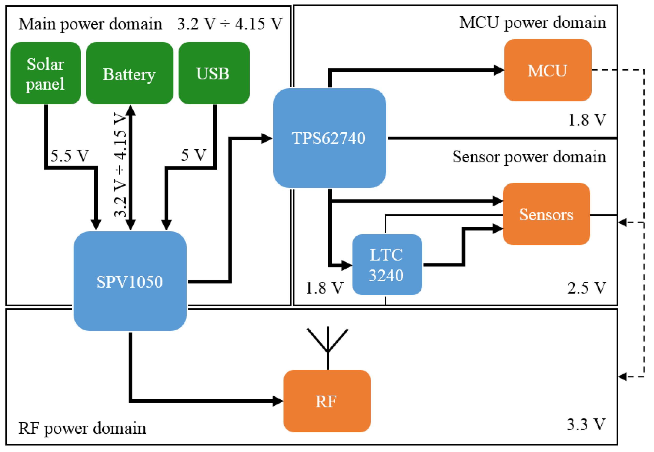
Integrated Circuits used in the device require 3 different voltage levels. Those are: 1.8 V as the MCU’s supply and all sensors’ digital voltage, 2.5 V as analog voltage for the UV-A and UV-B sensors and 3.3 V as the ZigBee module’s supply. Moreover, there is a primary 3.2 V ÷ 4.15 V supply which corresponds to the battery voltage and performs supply to the entire board. Therefore, power supplies were defined as domains:

• The main power domain (3.2–4.15 V), which is required to be present for the device operating;
• The MCU power domain (1.8 V), which is also required to be present for the device operating;
• The sensor power domain (1.8 V and 2.5 V), which can be enabled and disabled by the MCU;
• The RF power domain (3.3 V), which also can be enabled and disabled by the MCU.

Figure 10 shows principle of the power management in a graph form.

A Li-Ion battery, which is essential to the device operating, was placed in the main power domain. It can be charged by means of the SPV1050 with any source. The “any” means that the source can be high impedance (if the source is unable to sustain voltage at the maximum duty cycle, e.g., with a solar panel) or low impedance (if the source is able to sustain switching at the maximum duty cycle, e.g., with a USB). The only limitation is a voltage range which has to be less than 5.5 V.

3.3. Energy Harvesting Solar Panel

For energy harvesting purposes, a solar panel was used. Due to low-power and small size of the device, the solar panel was selected to suit these requirements. Features of the solar panel provided by the manufacturer are as follows:

• Maximum power: PMAX = 0.4 W;
• Open circuit voltage: VOC = 5.5 V;
• Size: 65 mm × 65 mm × 3 mm.

Unfortunately, the manufacturer did not deliver more information. Additional information such as the voltage–current characteristic is required to take advantage of the solar panel in the most efficient way. Thus, the data were achieved through measurement. The measurement circuit is presented in Figure 11.

The measurement was made by acquiring voltage and current signals in the time domain. The exemplary screenshot in Figure 12 shows the process of decreasing load from 10 k$\Omega$ to near 0 $\Omega$, where the additional math function of power was performed. The function was calculated from Equation (1).

$$P\left(t\right)=U\left(t\right)\times I\left(t\right)$$

(1)

A power function is required to acquire the Maximum Power Point (MPP), in which the solar panel works in the most efficient way.

The measurement consists of 3 datasets. The measurements were performed under artificial light exposure. Measured data were imported to the MATLAB environment in order to define electrical characteristics in detail. However, the raw data had to be prepared before arriving at the conclusion. The unpreparedness was a result of the measurement method. As was mentioned above, a digital oscilloscope performs measurements in the time domain, while the target domain is voltage. The voltage is not a monotonic waveform due to manual setting of the load at potentiometer as well as occurring noise. The Figure 13 shows the exemplary voltage–current characteristic created from raw data.

To make the data useful, signal processing had to be performed. It contained two steps:

• Making the voltage dataset monotonic.
• Filtering current signal.

The first step was to remove the sample of voltage $U\left(i\right)$ and $I\left(i\right)$ current if the previous voltage $U(i-1)$ sample was lower. This method left samples that fulfill statement (2) only:

$$U\left(i\right)<U(i-1)$$

(2)

If the statement is not met, the $U\left(i\right)$ and $I\left(i\right)$ samples are removed from the dataset. After performing this operation, the voltage dataset was monotonic.

The second step was to filter the current datasets by means of the Finite Impulse Response (FIR) low pass filter. The cutoff frequency and the filter order was set to 5 Hz and 200, respectively. These prepared data from 3 measurements was used to create 2 kinds of characteristics:

• Voltage–current (Figure 14).
• Voltage–power (Figure 15).

The voltage–current characteristic is a commonly used curve that provides detailed information about performance of the solar panel. The voltage–power characteristic was performed to determine the MPP of the solar panel. It was calculated from Equation (3).

$$P\left(U\right)=I\left(U\right)\times U$$

(3)

In the plots from Figure 14 and Figure 15, each curve represents one dataset of solar panel characteristics under artificial light. Black X-marks indicate the VMPP for each curve. Coordinates of those points are listed in

Table 2. The MPP measurement results for 3 datasets.

No. of Dataset	${\mathit{V}}_{\mathit{MPP}}$ (V)	${\mathit{MPP}}_{\mathit{ratio}}$
1	4.24	0.77
2	4.30	0.78
3	4.29	0.78

.

In order to provide the highest performance of the solar panel, operating voltage should be as close to $V_{MPP}$ as possible, i.e., in range from 4.2 V to 4.35 V, which corresponds to the $MP{P}_{ratio}$ from 0.76 to 0.79.

After familiarizing with the $V_{MPP}$ and the maximum power value provided by the manufacturer, the maximum available current can be estimated from Equation (4):

$$I_{MAX}=\frac{P_{MAX}}{V_{MPP}}=\frac{\left(0.4\mathrm{W}\right)}{\left(4.28\mathrm{V}\right)}=93\mathrm{mA}$$

(4)

3.4. Communication Parameters

All network parameters are programmed in each XBee module; thus, the MCU software is omitted in this area. This solution provides independence of the measurement and network section of the WSMs. Therefore, adding new devices or managing the existing ones is simplified. For programming the network nodes, Digi XTCU v6.3.2 was used. It is dedicated software for XBee modules. The considered network topology is mesh topology. Therefore, the routing path is dynamically established in order to find the shortest way to the destination node. This solution protects network reliability in the case of unreachability of some of intermediate nodes, for instance due to power-down of one of the routers. The process of establishing routes between source and destination devices is called route discovery. Coordinators and routers can participate in it. Network topology was tested with regard to the presence of the intermediate node which was the ZR. In Figure 16, the case with the ZigBee Router (ZR) was presented, whereas in Figure 17 the case without the ZR is shown. The network topology was rearranged automatically by the coordinator. In both cases, data transmission was successfully performed.

Adding subsequent routers to the network can provide enlargement of the system range to significant distance. The device specification shows that 400+ node networks are possible, which theoretically provide a range measured in kilometers.

Due to the fact that all data are directed to a single device, which is the ZigBee Dongle, the many-to-one routing approach was selected. This approach of routing is established by the setting time interval at the AR parameter for sending the many-to-one broadcast transmission by the data collector. The request has to be sent periodically to update the reverse routes in the network. Since the WSMs perform measurement every 10 min, the parameter was set to 0x1E (measured in 10 s units), which means the reverse routes are updated every 5 min.

To ensure the lowest current consumption of the XBee modules, I/O pins should never be left floating. Therefore, the unused I/O pins were set to outputs with a low logical level. Moreover, the transmit output power for the WSMs is limited to +1 dBm by means of disabling Boost Mode. However, the ZigBee dongle is set to provide full power.

The test lasted for about 2 h with a successful result. Achieved data are presented in the real-time plots in Figure 18. Each measurement is saved with its exact time of arrival at a PC.

3.5. Current Consumption of the ZigBee End Device

A lifetime estimation of the device required measurement of a current consumption. The device works periodically. Therefore, in order to receive full overview of the current consumption, measurement of one period is sufficient. Figure 19 presents current consumption in 3 states of the WSM work. When the sensor power domain is enabled, measurements are performed. This section lasts for 300 ms. Maximum current consumption is about 4 mA. The second section shows current consumption during the process of communication that includes powering the Xbee module, searching and joining determined network as well as sending the measured data. Moreover, in this section the System CPU is in active mode which also has an influence. The process lasts for about 570 ms. The time can vary depending on the result of the network finding. Current consumption of this section is critical for the device lifetime due to the amount of required energy. It is about 35 mA during transmitting and 8.5 mA in an idle state of the Xbee module. The last section concerns the sleep state of the device and fill the rest of the time which is about 9 min and 59 s in every cycle. Current consumption in this state was determined in 3 measurements with the use of Keysight Technologies 34461A high precision multimeter (Santa Rosa, CA, USA). Results are presented in

Table 3. Current consumption during sleep state of the WSM—measurement results.

Number of Measurement	Current Consumption (Average)
1	7.824 $\times {10}^{-6}$ A
2	7.966 $\times {10}^{-6}$ A
3	7.876 $\times {10}^{-6}$ A
Average:	7.889 $\times {10}^{-6}$ A

. The exemplary waveform of the current consumption is presented in Figure 20. An average current consumption during sleep state was assumed as 7.9 $\mathsf{\mu }$A.

Lifetime estimation started from calculation of the integral of the current consumption in time at active and sleep state separately. The active state current consumption result was separated and is presented in Figure 21.

The total active state charge was calculated from (5).

$$Q_{active}={\int }_a^{b}I\left(t\right)dt=\frac{b-a}{2N}\sum _{n=1}^N(I\left(t_n\right)+I\left(t_{n+1}\right))=0.00467 \mathrm{C}$$

(5)

$$\left[\mathrm{mAh}\right]=\frac{\left[\mathrm{C}\right]}{\left[\mathrm{s}\right]}\times 3.6\left[\mathrm{s}\right]=3.6\left[\mathrm{C}\right]$$

(6)

$$Q_{active}=3.6\times 0.00467 \mathrm{C}=0.016812 \mathrm{mAh}$$

(7)

The result of the charge amount used during the state is equal to Q = 0.00467 C. The unit that is more suitable for comparing with battery capacity is mAh. The result unit can be converted with the use of Equation (6). According to Equation (7), the charge is equal Q = 0.016812 mAh. Amount of consumed charge during the sleep state was calculated with the use of the average value of current and time of the state. The result provided by Equation (8).

$$Q_{sleep}=I_{avg}\times t_{sleep}\times 3.6=7.889\times {10}^{(-6)}\mathrm{A}\times 599\mathrm{s}\times 3.6=0.017\mathrm{mAh}$$

(8)

Therefore, total consumed charge within 10 min was calculated from Equation (9).

$$Q_{total}=Q_{active}+Q_{sleep}=0.0338\mathrm{mAh}$$

(9)

The last step was to calculate the total consumed charge during the course of a day in order to deduce if the device is able to work as long as required. The minimum lifetime for 1 battery charging is 24 h. Assuming that solar panel is able to fully charge the battery, the device is estimated to work as long as required without intervention. The whole day of the device’s operating consumes the amount of charge calculated from Equation (10).

$$Q_{day}=24\mathrm{h}\times 6\frac{1}{h}\times Q_{total}=4.8672\mathrm{mAh}$$

(10)

Total consumed charge during the course of the day is less than capacity of the battery (120 mAh); therefore, the condition is met. The estimated lifetime of the device without the external energy source is about 24 days.

4. Methodology of Prediction

The following sensor measurements were the input data for the predictive system:

• Temperature;
• Humidity;
• Atmospheric pressure;
• Sensor indications of PM10, PM2.5 and PM1 (separately);
• Noise level;
• Wind speed and direction.

The data aggregated by a single platform was clustered into 7 process variable vectors in 3 data sets (PM1, PM2.5 and PM10 separately) and then sent to the master node. The data were not neurally processed in WSM, but rather sent to the master processor. The acquired data (Figure 22) were archived in a .csv file, where the timestamp was stored in the unix format. The data range from the beginning of the measurements on 29 January 2017 to 7 May 2019 was selected for further processing and analysis.

The data were then grouped into a 3D array of 24 × 7 × 5 where each 24 × 7 array was a combination of all the readings from one day, and each subsequent layer corresponded to the preceding days. The data prepared this way were used for training both classical neural networks and deep learning networks. In addition, a data set with daily averages of measurements was prepared, which was used for teaching classical neural classifiers as well as regression networks and time series prediction networks. On the basis of daily averages, separately for PM10, PM2.5 and PM1 particles, permissible levels were determined with the application of the Directive on ambient air quality and cleaner air for Europe (OJ EU.L.2008.152.1 from 11 June 2008) and individual days were categorized depending on exceeding permissible levels of PM10, PM2.5 and PM1 particles.

4.1. Classical Neural Classifiers

The objective of the classification was to determine, based on the previous 5 measurement days and current measurements, whether the PM10 particulate matter permissible level would be exceeded in five days. The MATLAB environment was used for learning, in which data processing was previously performed. In order to preliminarily determine the best performing classifiers, basic types of classifiers were trained without structure optimization. The following machine learning methods were tested in a first series of tests: decision trees, discriminant analysis, logistic regression, naive Bayes classification, support vector machines, k-nearest neighbor classifiers and some ensembles classifiers. The classifiers which obtained the best results were then selected and training of these classifiers with parameter optimization was performed. KNN, optimizable ensembled, SVM and discriminant analysis classifiers were used in this part of testing.

The experimental results listed in the article fitting all the data. We did not do any modification, any erasing of existed data or extrapolation missed data. Deep learning methods were using raw data. The data division were 70% for training, and 30% for testing. In order to protect models from overfitting, an external testing set was used. In some algorithms, cross-validation was used as overfitting protection. Leave-one-out as well as k-fold methods were used. Leave-one-out is an exhaustive method of cross-validation which means it utilizes all combinations of training and testing data, it uses one sample for validation and other samples for training. On the contrary, k-fold is non-exhaustive method of cross-validation which means that not all combinations are used. K-fold [48] randomly splits dataset into k subsets and uses one as validation and the rest as training [49].

4.2. Deep Learning Classifiers

After testing the selected classical classification methods several times, it was decided to test deep learning classifiers. For simplicity of learning and lower data requirements, the Alexnet structure was chosen. The structure of the layers was adapted to the available data. Learning of the network took place on a computer equipped with a Nvidia RTX 2070 SUPER 8 GB graphics card.

Several prediction scenarios were conducted. First, neural prediction was performed for all input data for each of the 5 platforms separately, and then the results were averaged. The above neural predictors were also built when the input data were retrieved from all platforms at once. In the next case, the prediction results of each neural predictor were compared for data from all platforms simultaneously and for all platforms without noise measurement. No external weather stations or weather forecasts were used because WSM is intended to operate on current data and self-generated historical data. For the Deep Learning methodology, a modified Deepinsight algorithm described by [50] was used. The part that was not changed from the original is the method of creating images from vector data. What has been changed is the decision system, which was based on the Alexnet approach. The neural system is described in more detail in [51]. The methodology of creating images from vector data is based on a special transformation that transforms a feature vector to a feature matrix. The position of each pixel depends on the similarity of the features. The algorithm used in this case was Kernel Principal Component Analysis. It is a nonlinear dimensionality reduction and feature extraction algorithm that exploits the spatial structure of multidimensional features. It allows the recognition of more complex hidden layers (distances between pixels created from data). This algorithm assumes that once the location of a feature is determined, it is possible to map the feature values. This results in a unique image for each feature vector. An example image from the measurement data obtained from the presented self-powered platform is shown in Figure 23. Such images were then used to teach Alexnet-type networks.

In the case shown in Figure 23, two rectangles and a set of pixels are shown. The points marked denote not the values for a feature, but only the locations of the features. The smallest rectangle containing all features (the black rectangle) is determined first. This approach reduces white noise in the data for the later neural-based reasoning system. For optimization purposes, the rectangle is rotated into a red rectangle using the convex hull algorithm. Only such an image is analyzed further by the neural network.

5. Results

First, the study was performed for PM10 particulate data using classical neural networks. The network learning results are presented collectively in

Table 4. Results for different neural networks without considering the noise level (PM10 variant).

Neural Network	Precision (%)	Recall (%)	Specificity (%)	Accuracy (%)	F1 Score (%)
KNN	92.85	83.87	94.87	89.99	88.13
NaiveBayes	100	48.38	100	77.14	65.21
OptDisc	84.37	87.09	87.17	87.14	85.71
OptSVM	84.84	90.32	87.17	88.57	87.50

and graphically in Figure 24 for KNN. The data in Table 4 were calculated based on known formulas for Precision (11), Recall (12) Specificity (13), Accuracy (14) and F1 Score (15) presented in [52].

$$Precision=\frac{TP}{TP+FP}$$

(11)

$$Recall=\frac{TP}{TP+FN}$$

(12)

$$Specifity=\frac{TN}{TN+FP}$$

(13)

$$Accuracy=\frac{TN+TP}{TN+FP+TP+FN}$$

(14)

$$F1Score=2\times \frac{Precision\times Recall}{Precision+Recall}$$

(15)

where:

• $TP$—true positives.
• $TN$—true negatives.
• $FP$—false positives.
• $FN$—false negatives.

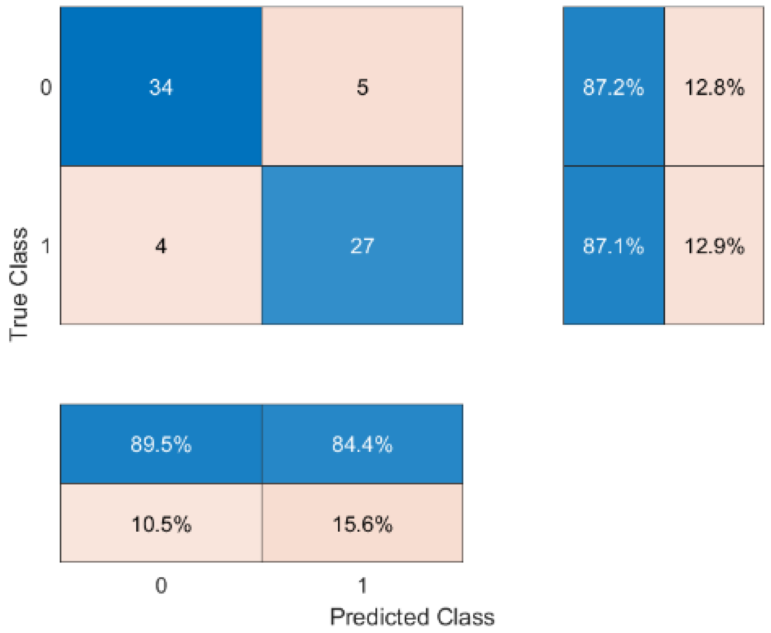
The first approach to analyzing the results was performed excluding the measurements from the noise sensor.

The field seen in Figure 24, which is at the coordinates of (0, 0) stands for True Negative, which indicates the number of negative (not having the feature) cases that were correctly detected. The field with coordinates (0, 1) indicates False Positive elements, which means elements which were negative but were classified as positive. The coordinates (1, 0) indicate False Negative items, which are positive items that were classified as negative. The coordinates (1, 1) indicate True Positive results, which are positive and correctly classified. The remaining fields, expressed as percentages, are the resulting percentages converted with True Positive and True Negative, or False Positive and False Negative, or calculated from True (Positive and Negative) or False (Positive and Negative).

The KNN network had the best Accuracy, while the NaiveBayes network had the worst Accuracy. The OptSVM network had comparable Accuracy to KNN. This can be explained by the fact that they are natively designed for classification tasks, whence may be their better usefulness in classifying whether the next day will be a PM10 air pollution exceedance day.

In the course of the work, it was detected that monitoring ambient noise can affect the accuracy of the predictions made by the neural networks. The results of network learning for such a case are presented in Figure 25 and

Table 5. Results for different neural networks including the noise level (PM10 variant).

Neural Network	Precision (%)	Recall (%)	Specificity (%)	Accuracy (%)	F1 Score (%)
KNN	88.88	91.42	88.57	90.00	90.14
NaiveBayes	73.52	71.42	74.28	72.85	72.46
OptDisc	88.23	85.71	88.57	87.14	86.95
OptSVM	91.17	88.57	91.42	90.01	89.85

. Interestingly, a slight improvement occurred only in the case of dedicated classification solutions, that is, for KNN and OptSVM networks. In the other cases, there was a deterioration in the results.

Next, the Deep Learning network was applied for the same data and scenarios as the classical networks.

Using the network with the algorithm to image the vector data improved the reasoning Accuracy, as shown in

Table 6. Accuracy for learning classical and DL type networks.

Neural Network	Data	Accuracy (%)
KNN	Without noise sensor	89.99
OptSVM	With noise sensor	90.01
Deep Learning	Without noise sensor	92.13
Deep Learning	With noise sensor	94.61

. Compared to the best KNN (without noise sensor) and OptSVM (with noise sensor) solutions, the DL solution was better by 2.14% and 4.60%, respectively. Interestingly, the DL network obtained a better result without the noise sensor than the classical network with additional noise sensor data.

A similar pattern can be observed by analyzing the data in

Table 7. Increase in Accuracy for learning DL networks over classical neural networks for different data sets.

Type of PM Measurements	KNN (%)	NaiveBayes (%)	OptDsc (%)	OptSVM (%)
PM10 without noise sensor	2.13	14.99	4.99	3.56
PM10 with noise sensor	4.61	21.76	7.47	4.60
PM2.5 without noise sensor	2.53	12.83	4.99	4.01
PM2.5 with noise sensor	4.81	22.03	7.55	4.95
PM1 without noise sensor	1.95	13.11	4.78	3.27
PM1 with noise sensor	4.58	20.80	7.17	4.52

. For each test and particulate variant, better Accuracy was obtained compared to the classical approach. For each type of particulate matter, the prediction of exceeding the acceptable concentration on the next day was better by several percent than the classical methods. A significant improvement in the results for the system with noise data can also be observed.

6. Conclusions

The project of the distributed wireless measurement system was realized with satisfactory results. The system is composed of the four executive units—WSMs and the coordinating unit—the ZigBee Dongle. The system measures environmental parameters, i.e., humidity, temperature, pressure, illuminance, UV-A and UV-B irradiance as well as wind speed and direction and air pollution. The system uses the RF ZigBee protocol to communicate wirelessly. The network topology is a self-healing mesh, which provides a reliable solution in the case of node failures. The WSMs are energy-independent due to the double-source power supply––a rechargeable battery and solar energy. The ZigBee Dongle connected to a PC via USB port coordinate the wireless network and provides easy data acquisition and processing in the MATLAB environment.

The ZigBee network was configured to meet the project’s assumptions of a self-healing mesh, and low-power construction of the system. The proposed concept can enlarge the network area to significant distances with multiplication of the network nodes. It can be achieved by using the router functionality of the WSM. In order to utilize measured data, an algorithm for data acquisition and processing in the MATLAB environment was developed.

Examination of the designed system is presented. Tests were performed in the field of power consumption and related lifetime of the WSM in both functionalities—as an end device and as a router. The estimated lifetime result of the WSM as the end device is about a month on a single coin battery without solar exposition. That makes the system a low-power construction. The tests included also confirmation of the energy harvesting capability, showing that the designed WSM is an energy-independent device. The final verification was the test, which confirmed the system as a whole work according to the assumptions.

As a result of the research work, the following conclusions were found:

• Among all the applied neural classifiers, the highest effectiveness was achieved by those belonging to the Deep Learning group. Networks of this type can independently explore relationships unknown to experts, and, thus, for large sets of input data, find hidden correlations between them.
• Array deployment of wireless sensors over a larger area can improve prediction performance already at the level of predictor architecture. Over the course of the research, it was shown that the effectiveness for the same data for averaging results from individual platforms is lower than for an inference system in which the network simultaneously covers data from all platforms.
• An unexpected result of the study is what effect noise measurement has by WSM. If the neural network also considers this parameter as an input parameter, there is an improvement in the performance of predicting the occurrence of air pollution exceeding established limits. In this way, the DL network indirectly discovered the relationship there is an increase in the use of combustion vehicles when the weather is worse. In this way, without using data from weather stations, it implicitly discovers increased combustion in urban traffic and low emissions, which impacts the increased probability of occurrence of air pollution exceeding established limits.

Further work will focus on the influence of the number and deployment of the platforms with the established neural network architecture on the quality of air pollution prediction. The optimal number of wireless sensor platforms will be determined in terms of economic aspects. The optimal number of platforms, whose increase will not significantly improve prediction efficiency, should be determined. Work will also be carried out on optimizing the energy consumption of a single WSM platform.