Article

A Novel Smart Charging Method to Mitigate Voltage Fluctuation at Fast Charging Stations

by
Sami M. Alshareef
Department of Electrical Engineering, College of Engineering, Jouf University, Sakaka 72388, Saudi Arabia
Energies 2022, 15(5), 1746; https://doi.org/10.3390/en15051746
Submission received: 4 February 2022 / Revised: 22 February 2022 / Accepted: 24 February 2022 / Published: 26 February 2022

Abstract

:
The research presented in this paper focuses on the impact of fast charging stations (FCSs) on voltage quality. When the operation of FCSs causes a voltage fluctuation and light flicker, the FCSs may be disconnected, as per the utility general standard practice, which results in financial loss represented by FCS downtime. FCS downtime can be avoided by mitigating voltage fluctuation and light flicker. Flicker mitigation devices that are available in the market are characterized by their high total annual equivalent costs. As an alternative, a novel smart charging method is proposed in this study in order to mitigate both voltage fluctuation and light flicker, whereby customers can select one of three charging services available in fast chargers: premium, regular, or economic charging power. The charging power is selected according to customer priority in relation to time and cost, which offers more flexibility than those currently available in the literature. For instance, the premium power can be selected if the time is more valuable to the customer at the time of arrival at the FCS; in contrast, the regular or economic power are utilized if the cost is more valuable than the time. The results reveal that when an FCS charges a vehicle by an uncontrolled charging method, the FCS violates the flicker tolerance especially when demand for its service is increased by 20% and beyond. In contrast, the flicker limit is not violated when vehicles are charged from an FCS as per the proposed smart charging approach, even when the penetration on the FCS is increased by 50%. The proposed smart charging method offers a compromise solution to satisfy several stakeholders with different interests. Thus, the system operator equipment, FCS investors, nearby customers, and owners of electric vehicles will not be impacted by integrating the FCSs into the distribution networks.

1. Introduction

1.1. Motivation

As the number of electric vehicles (EVs) increases, fast charging becomes a necessity in electric service stations, not only to reduce charging and waiting times for EVs, whether in service or in a queue, but also to increase their commercial benefits by increasing their utilization rates. Fast charging stations (FCSs) are extremely important in reducing downtime due to charging, especially for ride-hailing EVs as well as commercial and automated car-sharing EVs. However, FCSs are characterized by their high power consumption from electric grids [1]. Power consumption is determined by the current drawn by EVs. The times and periods of that consumption are indeterminate due to several uncertain parameters that are inherent in the EV charging process, such as their numbers, battery capacities, state-of-charge levels at the time of arrival, as well as their actual time of arrival, all of which may lead to a degradation in the voltage quality of electric power. Voltage fluctuation may happen when repeated and sudden changes occur in the real and reactive power that is drawn from FCSs by EVs. As per the utility general standard practice stated in [2], it is not permitted to cause any voltage fluctuation in the system, since this could lead to light flicker for nearby customers. If flicker emission levels are violated by the operation of customer equipment, the network operator may require [3,4]: mitigative action taken by the customer; a disconnection of the customer’s equipment until mitigative action can be taken; and/or a possible service disconnection of the fluctuating facility. It is the responsibility of the facility owner/operator to limit voltage fluctuation caused by the operation of their equipment [3]. As illustrated in Figure 1, from the viewpoint of the investor, the main benefit of flicker mitigation is to avoid service disconnection on the facility. The utility point of view is to protect both equipment as well as nearby customers. When the operation of FCSs causes a voltage fluctuation and light flicker, the FCSs may be disconnected, resulting in financial loss, represented by the FCS downtime. The downtime is the total amount of time that the FCS is not accessible. The FCS downtime and its losses can be interpreted as the cost of voltage flicker incurred by the FCS’s owner. To avoid FCS downtime, voltage fluctuation and light flicker should be mitigated.

1.2. Related Works

The subject of smart charging has been addressed in recently published key works and from different aspects, the aim of which includes minimizing: the system peak [5]; the imported energy by the local operator [6]; the local distribution company’s operational costs [7]; the total feeder losses [8]; and the waiting time in queue at the charging station [9]. The node type of the charging station (fast or slow) is a PQ-bus. By controlling the active power (P), the aforementioned objectives in the literature have been achieved. However, to control the voltage fluctuation in a PQ-bus without a mitigation device is an interesting concept. While the voltage in a PQ-bus is a state variable and depends on the drawn active power, it is an FCS and the drawn active power is controlled by parameters that are controlled by customers, such as the required level of charge, which affects the duration, the arrival time, and the number of vehicles served from the station. Unlike home or fleet charging at night where vehicles park for long periods, thus creating flexibility to regulate the drawn power, the FCS is required to deliver the power in a very short time, as determined by customers. The difficulty is how to control the voltage and reduce the fluctuation in a PQ-bus without injecting a reactive power. The related works in the literature are compared according to three aspects: the charging power; the smart charging approach; and the reported flicker value. Previous work can be classified broadly into four groups, the first of which considers uncontrolled and/or smart charging via a slow charging station (i.e., a home charger). The second group applies the uncontrolled and/or smart charging but via a fast charger (i.e., an FCS). Neither of these two groups studies the impact of the charging station on voltage fluctuation and light flicker. The third group analyzes the impact of voltage fluctuation on light flicker whereas the fourth group of studies addresses and mitigates voltage fluctuation and light flicker by costly mitigating devices. Nevertheless, the source of the flicker in the last two groups is not the charging stations but rather conventional loads such as an arc furnace or a rolling mill. The goal of the work presented in this paper is to fill the research gap by addressing the impact of an FCS on voltage fluctuation and light flicker, and mitigating that impact using a novel smart charging approach that has not been previously utilized, to the best of the author’s knowledge. Table 1 presents a comparison of the method proposed in this paper and other existing studies. Table 2 illustrates the impact of charging EVs according to the method and type of electricity systems, as per the previous work as well as the proposed smart charging method. Smart charging is a method of optimizing the charging process to facilitate the integration of EVs while meeting any constraints of the distribution system as well as customer preference.
The current concept of smart charging available in the literature, which is listed in Figure 2, encompasses different levels of control over the charging process, aiming to support the power system by achieving different objectives. In this study, the proposed smart charging targets the future smart grid. It is assumed that the same port (nozzle) of the fast charger is able to provide three different charging powers, namely, economic, regular, and premium. The rate of charging in each charging power is defined by the FCS operator/investor and can be changed within the day according to different variables such as on-/off-peak hours and the local level of produced renewable energy.
Unlike smart charging in the previous work [6,7,8,9,10,11,12,14], customers can select the charging power in the proposed smart charging method according to their value of time and cost. At the time of arrival at the FCS, if time is the most important consideration for a customer, the premium charging power can be selected. In contrast, if a customer prioritizes cost, regular or economic charging power can be utilized. Unlike the previous work related to smart charging in which only system conditions, such as peak shaving, grid congestion, and ancillary services, are considered, the proposed smart charging also considers the customer’s priority in relation to time and cost. Moreover, the proposed charging method introduces market competition among different fast charging providers to offer competitive rates of charging as well as competitive pricing for each charging power.

1.3. Contribution

The study conducted in this paper quantifies and mitigates the adverse effects of FCSs on voltage fluctuation and light flicker. The list of key contributions are as follows:
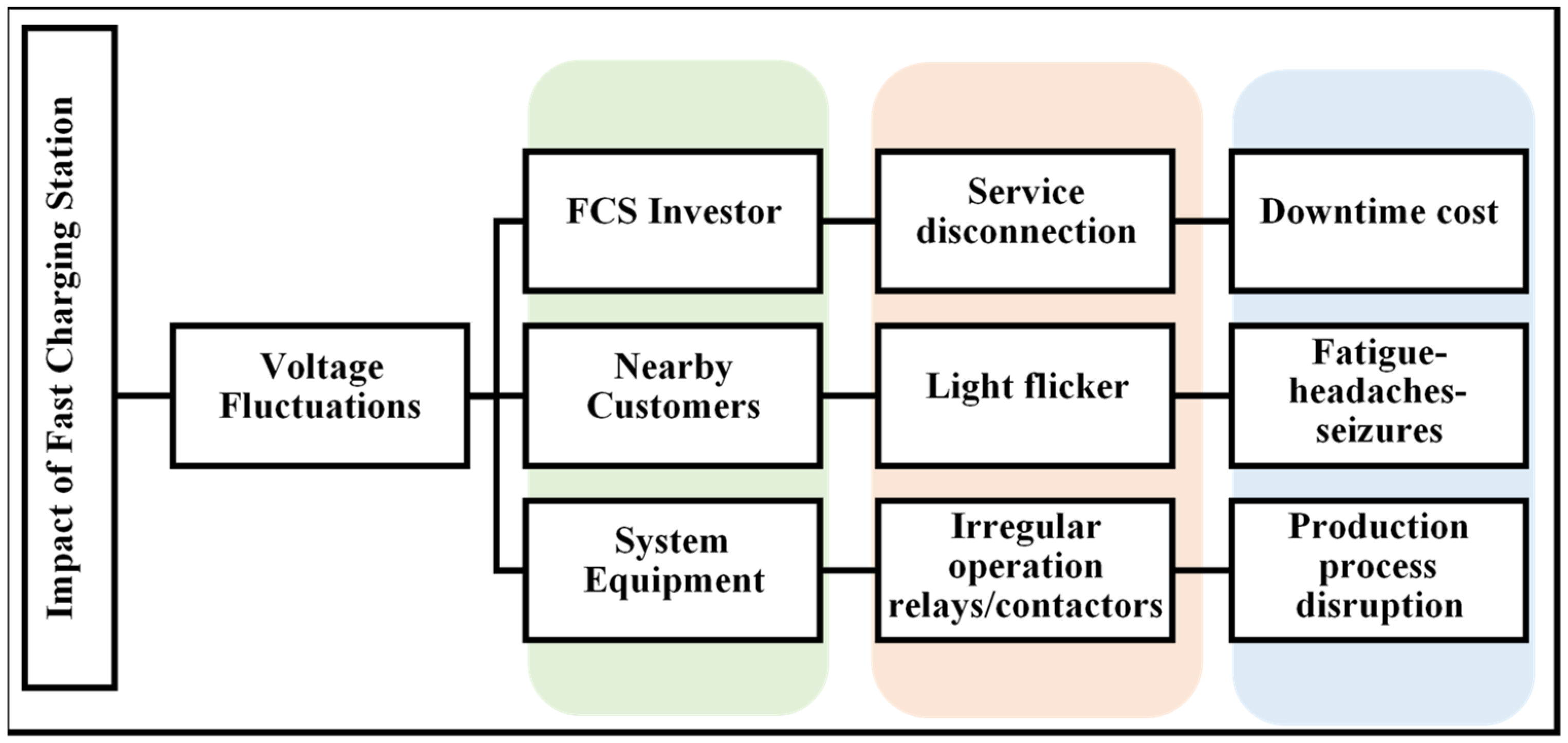
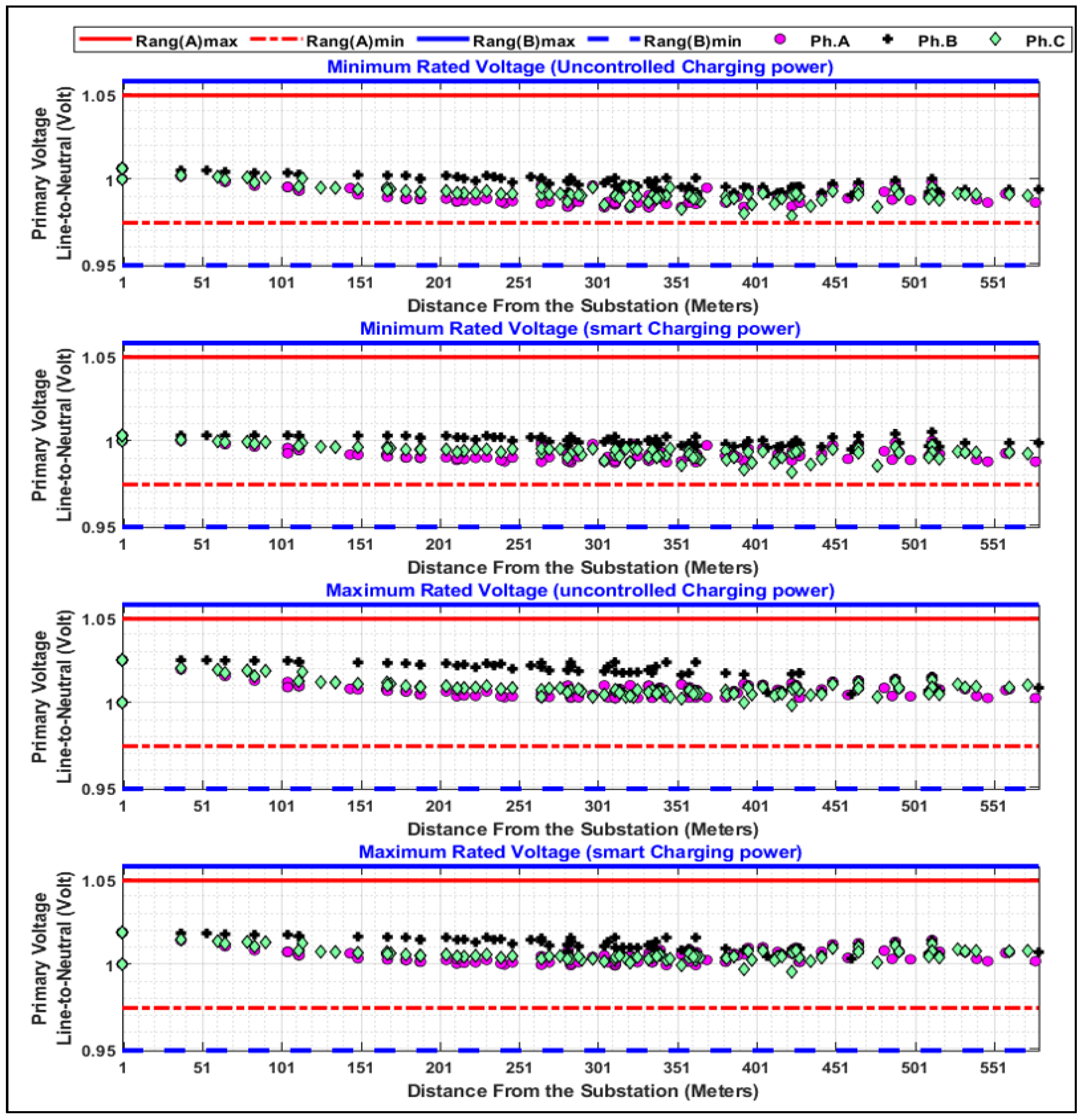
  • Investigation of the quality of the service voltage in the presence of FCSs in distribution grids;
  • Proposal of a novel smart charging approach that quantifies and mitigates the impact of an FCS on voltage fluctuation and light flicker;
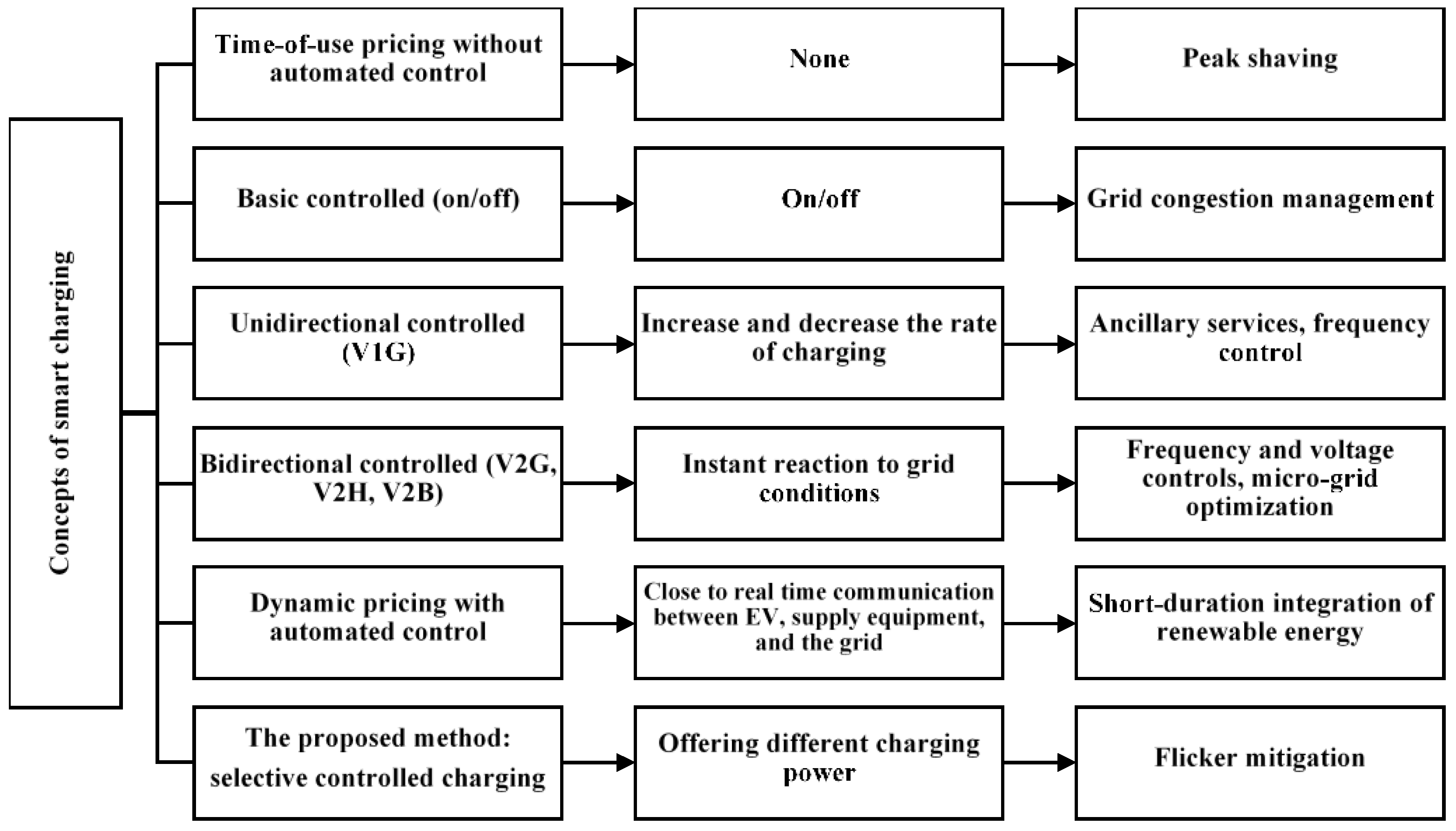
  • Development of a novel set of smart charging constraints that offers more flexibility to customers than those currently in the literature, and by which customer can select the charging power according to priority of time or cost.

2. Input Data Required for a Vehicle Charging Model

2.1. Number of BPEVs

The number of EVs in the system, N B P E V , is determined as in (1) and is a function of the number of houses in the system and number of vehicles in each house. It is assumed that there are two vehicles per house. A share of N B P E V requires battery charging using FCSs.
N B P E V = x p e n · n h o u s e · n c a r
where N B P E V is the number of EVs in the system, x p e n is the share of EVs with respect to the total number of vehicles in the system, 10–50%, n h o u s e is the number of residential houses in the system, and n c a r is the number of vehicles per house.

2.2. Types of BPEVs, Their Shares, and Locations

Figure 3 shows shares and charging locations for three types of vehicles. Battery powered electric vehicles (BPEVs) are classified based on their battery capacity μ into BPEVs with: small battery capacity μ s ; medium battery capacity μ m ; and large battery capacity, μ l . Therefore, there is V s number of BPEVs in the system with a small battery capacity μ s . The battery capacity limit of each v V s is as Formula (2).
μ s 50   kwh
Furthermore, there are V m and V l numbers of BPEVs with medium μ m and μ l large battery capacities in the system.
50   kwh < μ m 100   kwh
μ l > 100   kwh
Each vehicle ν in the system can charge using a home charger, V H o m e , or FCS, V F C S .
V s = { V F C S s V H o m e s }
V m = { V F C S m V H o m e m }
V l = { V F C S l V H o m e l }
V = { V s V m V l }
V F C S = { V F C S s , V F C S m , V F C S l }
Assumptions:
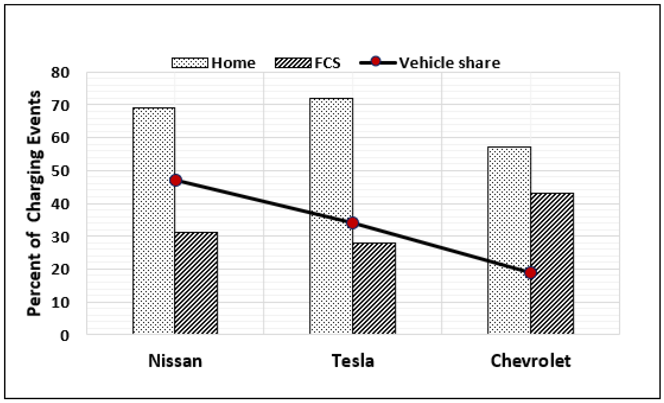
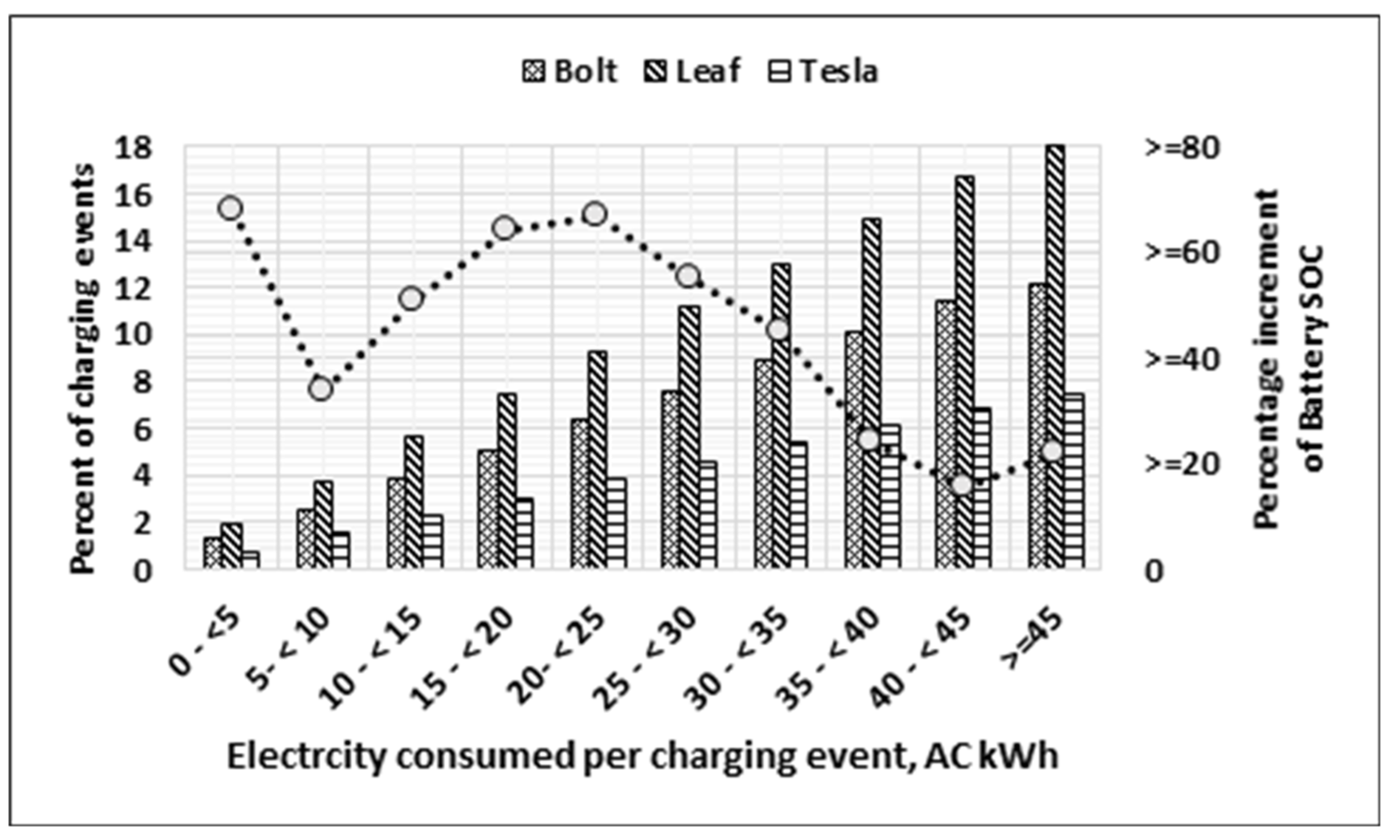
  • Three different BPEVs are utilized in the system because of their high market shares representing more than 50% [25]. These vehicles are the Tesla Model S, the Chevy Bold, and the Nissan Leaf;
  • The Nissan Leaf is assumed to represent the group of BPEVs V s with small battery capacity, μ s ;
  • The group of BPEVs V m with medium battery capacity μ m is represented by the Chevy Bolt.
  • The Tesla Model S is utilized to represent the group of BPEVs V l with large battery capacity, μ l .
The aforementioned vehicles charge from home and public charging stations. It is assumed that all public charging stations in [26] are FCSs. This seems to be a realistic assumption for the following reasons:
  • As battery prices decrease, the battery capacity increases, thus it would not be sufficient (if there were a willingness and need) to charge the vehicle from slow charging stations;
  • The EV market share is forecast to be 50% by 2030 [27]. As the BPEV market share increases, public charging stations need to meet the increased share by increasing the utilization rate. This is not achievable by assuming slow charging stations;
  • Considering the value of charging time, especially for ride-hailing EVs, as well as commercial and automated car-sharing EVs, FCSs are extremely important in reducing downtime due to charging.

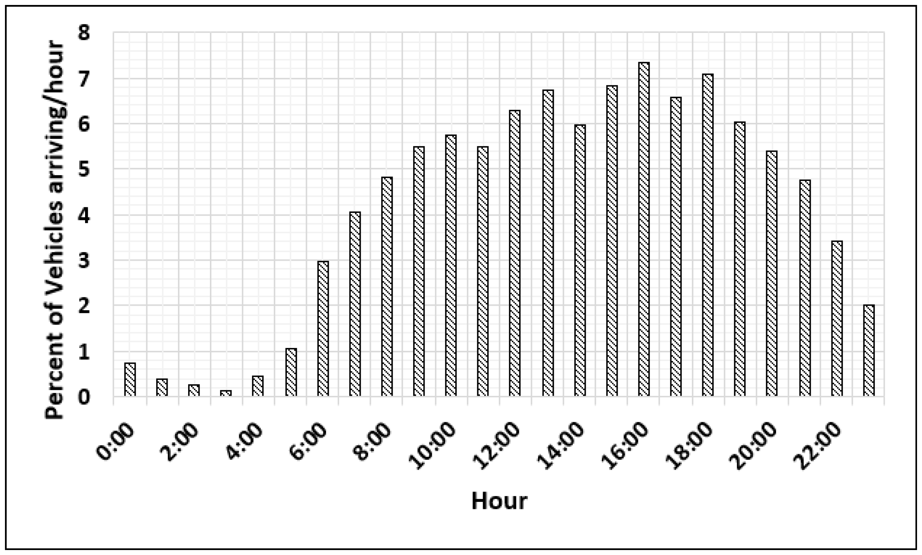
2.3. BPEV Arrival Rate at FCSs

Figure 4 depicts a probability distribution of vehicle arrival rate and time at the FCS prior to charging [28]. The probability distribution is utilized to estimate the arrival rate according to their arrival time at the FCS by a Markov Chain Monte Carlo (MCMC) simulation. The Birnbaum–Saunders distribution function is selected to be the best distribution that fits the distribution shown in Figure 4. [25]. MCMC is utilized to sample the selected distribution. The output of MCMC indicates the hourly arrival rate at the FCS, which represents the start of charging at the FCS.

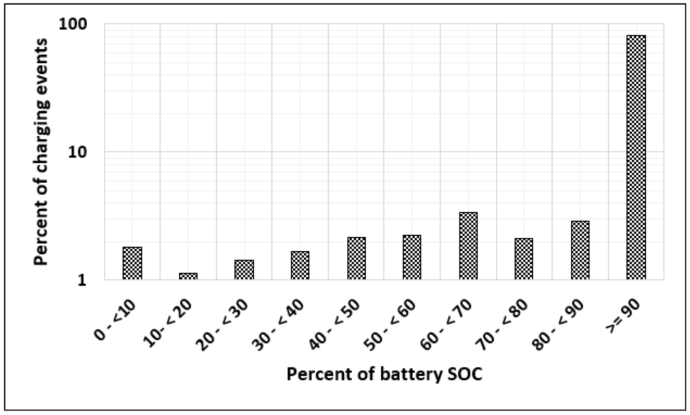
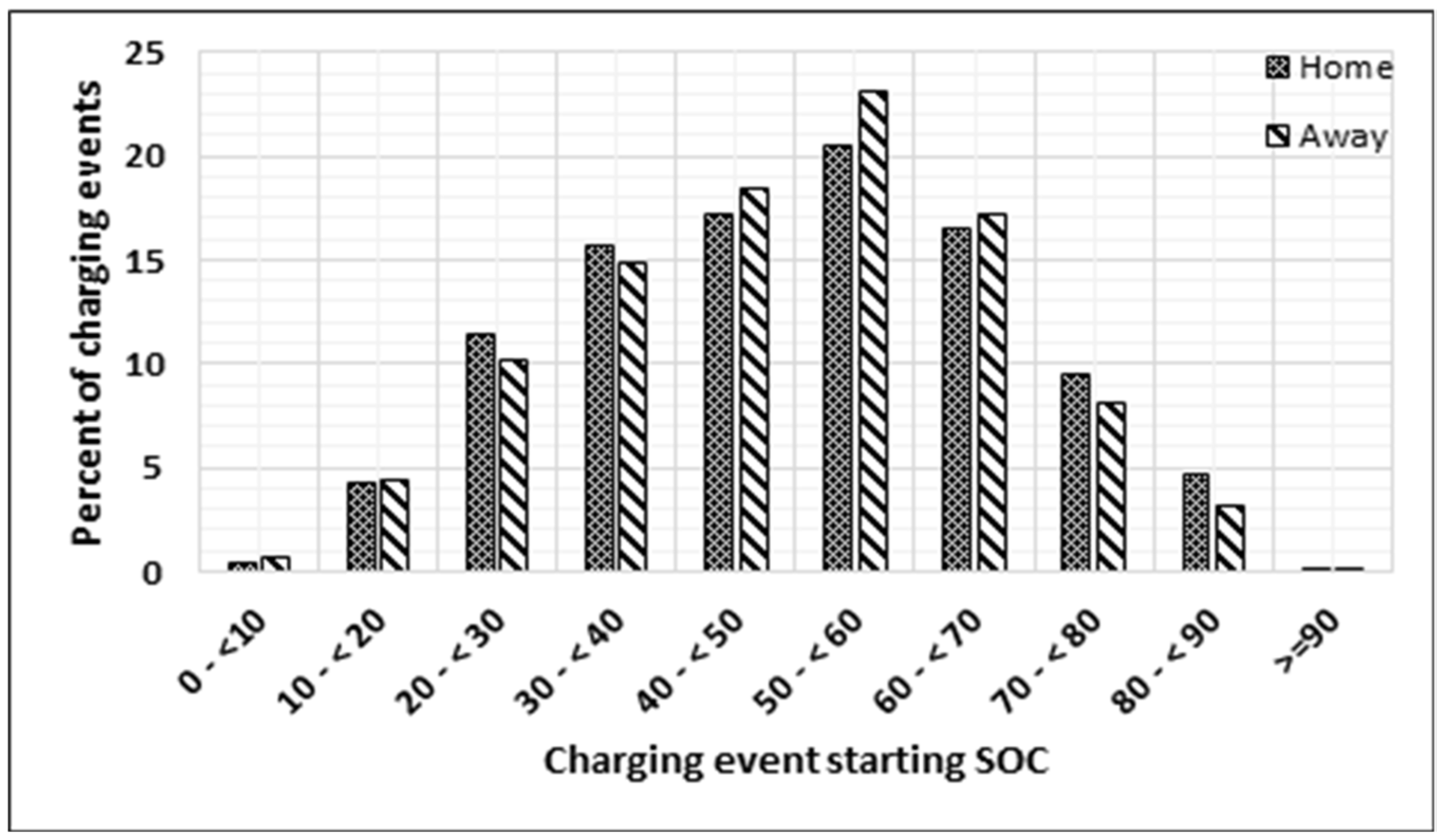
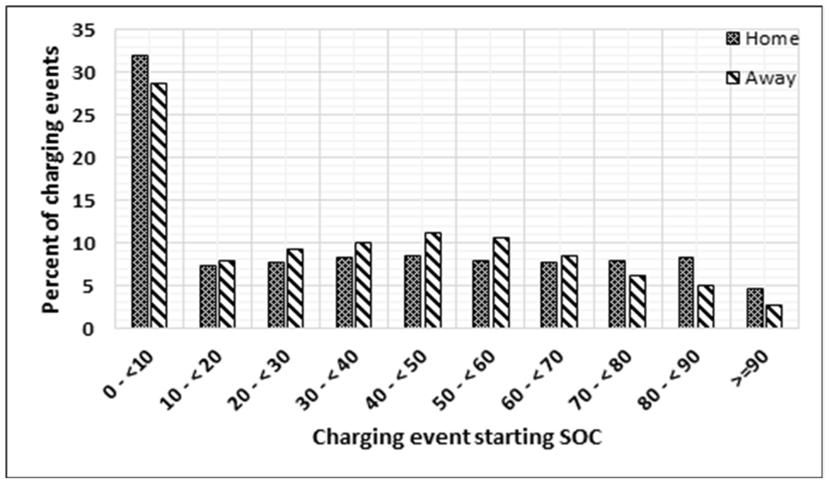
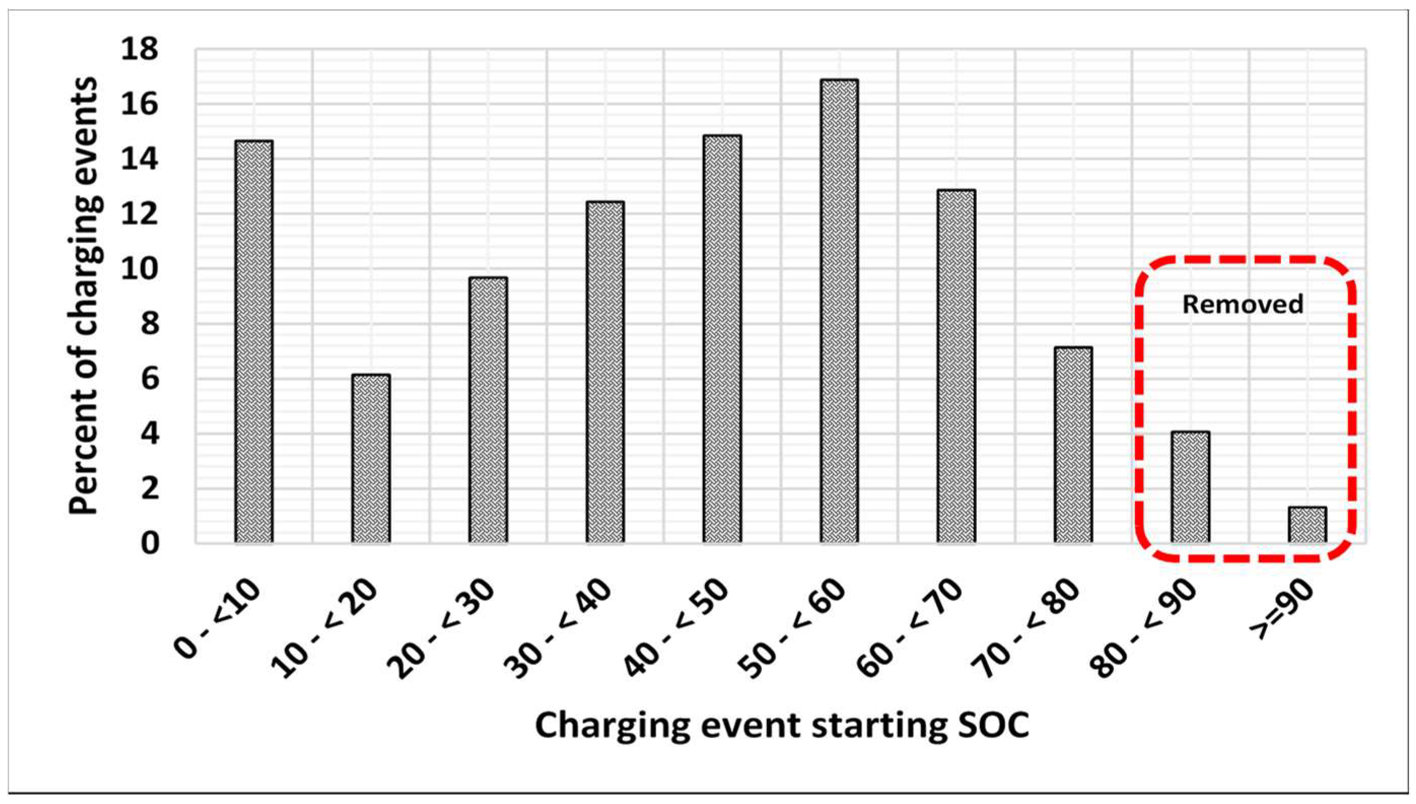
2.4. Level of Batteries Charged Form an FCS

When any vehicle v V starts a trip, it most often begins from home. Most of these vehicles start with an almost fully charged battery, according to the distribution shown in Figure 5. Some of these vehicles,   v V F C S , are required to charge away from home. Based on the assumptions stated above, it is assumed that charging events at away-from-home charging locations will occur at an FCS; thus, their corresponding probability distributions represent the level of charged batteries at an FCS. The probability distributions from Figure 6 and Figure 7 are averaged as in Figure 8 to depict the state of charge (SOC) level at the time of arrival at the FCS for the three types of vehicles mentioned above. At an FCS, vehicles are not permitted to charge more than 80% of their SOC [29]; thus, Figure 8 shows the removed percentage of charging events of 80% SOC and up.

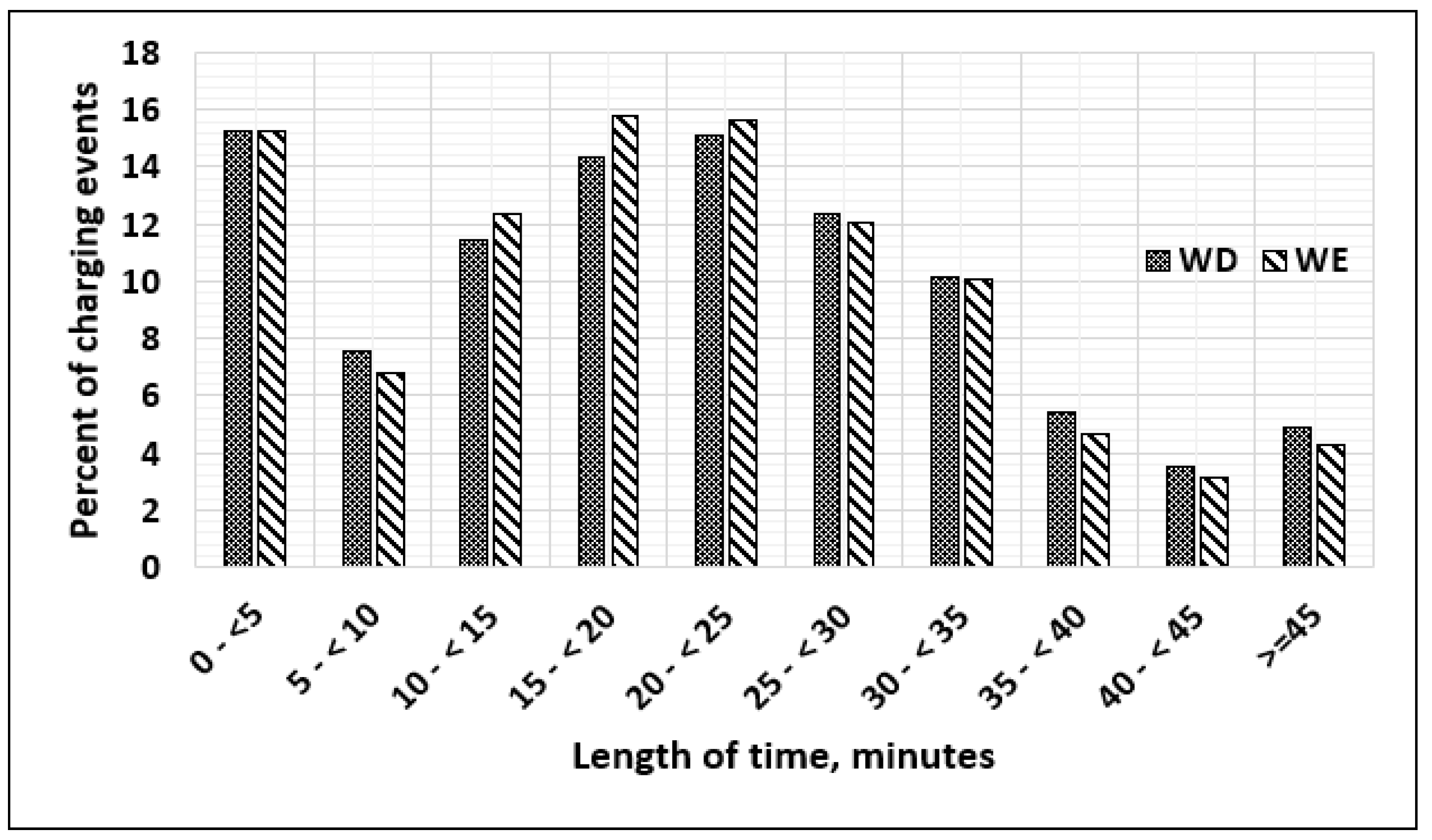
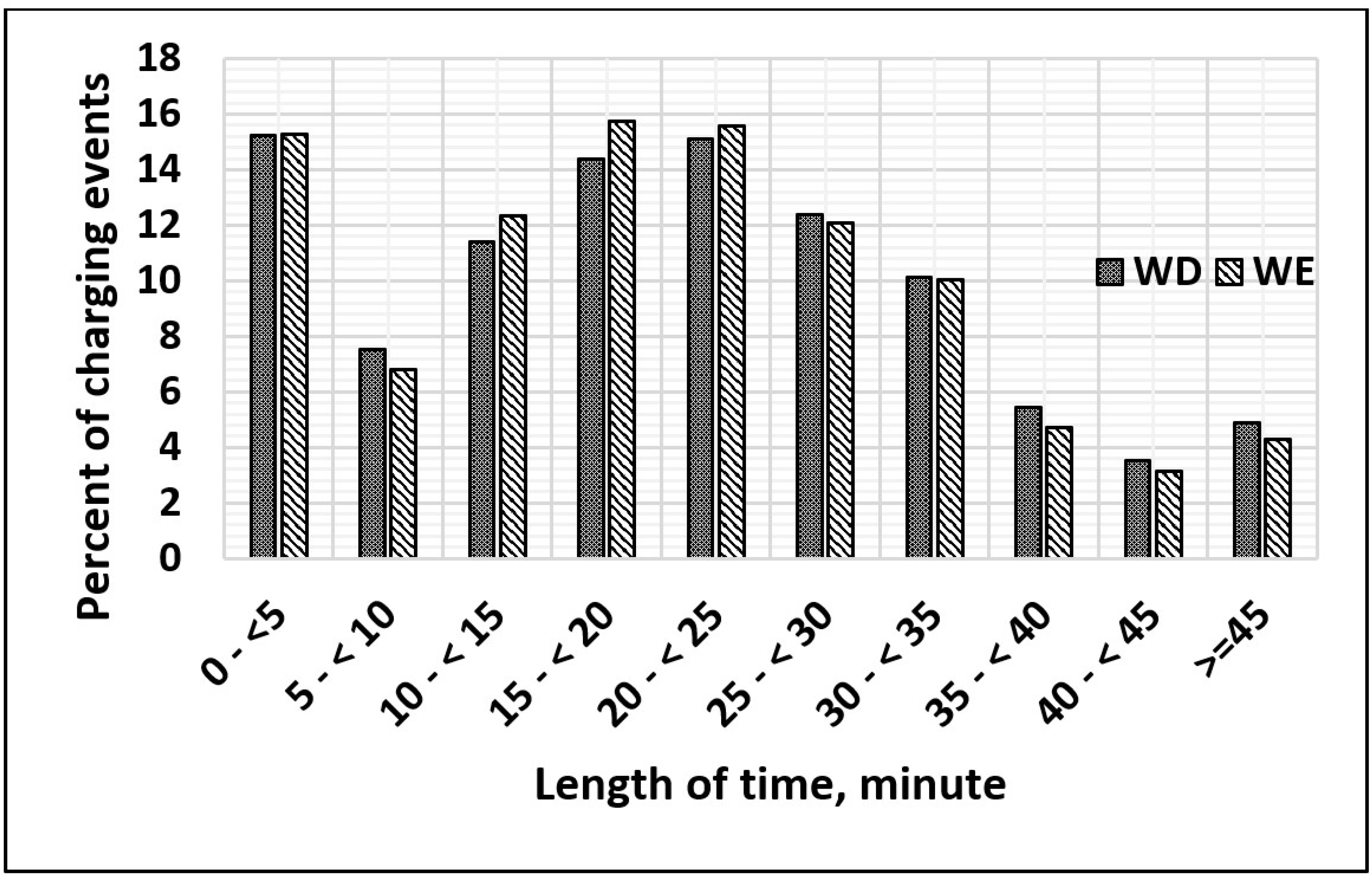
2.5. Length of Time for BPEVs to Draw Power Form an FCS

At this point, types of vehicles are specified, and their share and charging locations are determined (Figure 3). Their arrival rate at the FCS (Figure 4) and level of battery charge when they arrive are depicted (Figure 8). In order to determine the energy required from the FCS for each charging event, Figure 9 is utilized to estimate the length of time for a vehicle to draw power from the FCS. Given the length of the charging event, the rated power β of an FCS, and the efficiency η F C S of the charger, the energy required from the FCS k w h F C S is estimated linearly, as shown in Figure 10, as follows:
k w h F C S = ( L F C S μ v β . η F C S . ϑ ) · μ v  
μ v : { μ s ,   i f   ν V s μ m ,   i f   ν V m μ l ,   i f   ν V l
where k w h F C S is the energy required for vehicle v from the FCS (kwh), L F C S is the length of time with the vehicle connected to the fast charger (minute), μ v is the battery capacity of vehicle v (kwh), η F C S is the efficiency of the fast charger (%), and ϑ is the factor to convert an hour into minutes. In Figure 10, the percentage increment of the battery SOC is added to the initial battery SOC recorded at the time of arrival. The length of time is randomly generated by Monte Carlo simulation to estimate the required energy from the grid. The minimum length of time with a vehicle drawing power from the FCS is assumed to be five minutes, as shown in Figure 9, for weekdays (WD); thus, the minimum kwh required from the FCS per any charging event is 4 kwh.

2.6. Length of Time for BPEVs to Be Connected to an FCS

At this point, the required energy from the FCS per charging event is determined; thus, the customer can be billed according to the energy consumed from the FCS. However, customers who use commercial charging stations are billed based on the length of time the vehicle is connected to the FCS, not the length of time the vehicle draws power from the FCS [32]. Therefore, Figure 11 is utilized to show if there is any variation in the length of time between when a vehicle is connected to or drawing power from an FCS. The distribution of the length of time a vehicle is connected to an FCS, per charging event (Figure 11), is nearly identical to the distribution of the length of time a vehicle is drawing power from the FCS, per charging event (Figure 10). It is assumed that the customer departs from the FCS when the vehicle is charged with the required energy. Therefore, in this work, the customer is billed only according to the electricity consumed per charging event.

3. Proposed Smart Charge and Mathematical Models
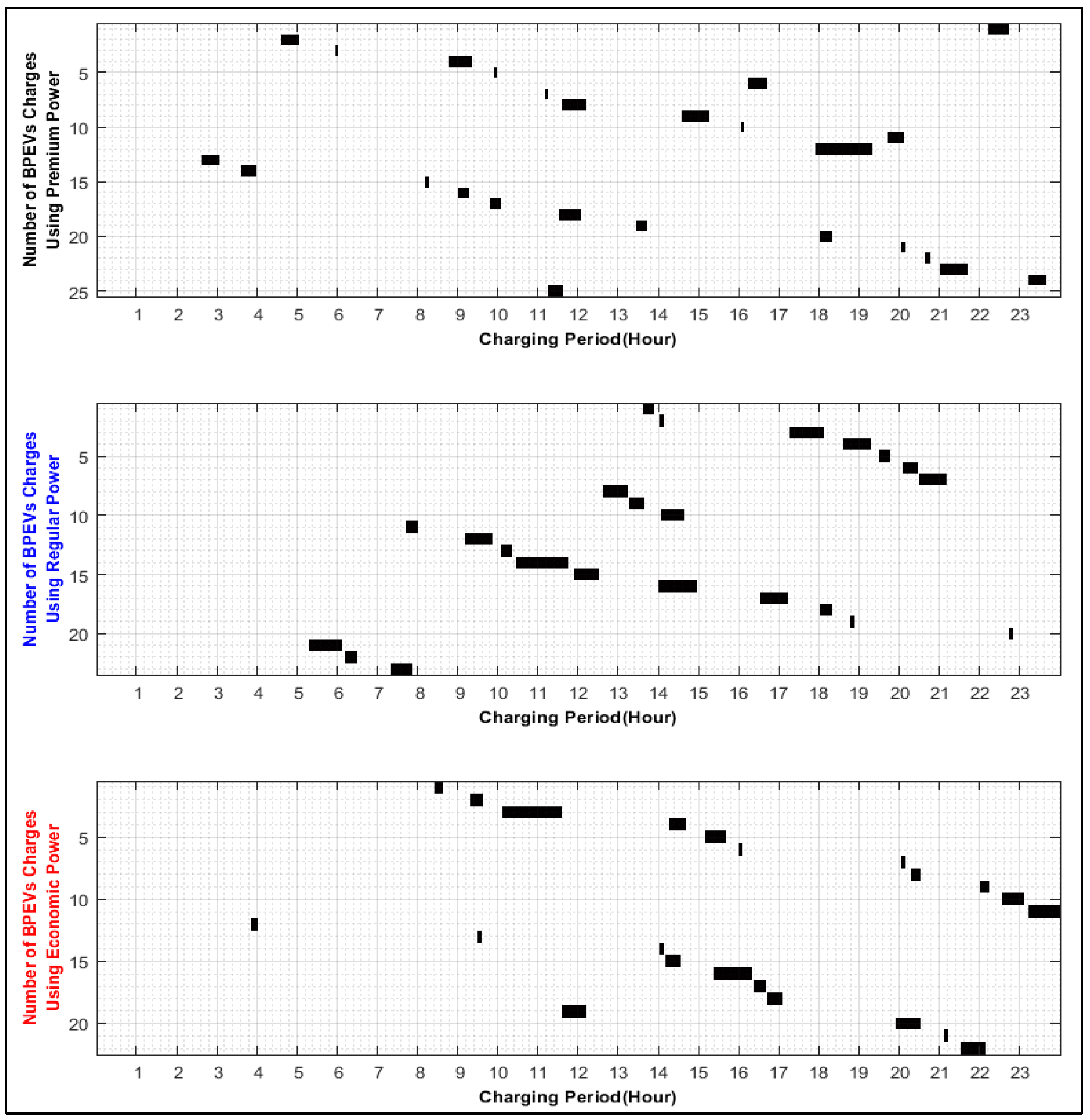
3.1. Charging Power

Uncontrolled Charging: The uncontrolled charging power β^u is equal to the maximum output power (β) of the charger. In this case, when a vehicle arrives at the FCS, it charges using the maximum output power of the FCS; thus, the charging duration is estimated accordingly.
Smart (Controlled) Charging: In this case, an FCS encompasses three charging powers:
  • Premium;
  • Regular;
  • Economic.
Premium charging power: can provide an EV with an output power ( β p ) ranging from p ¯   % to p ¯   % of the maximum output power β .
Regular charging power: can provide an EV with an output power ( β r ) ranging from r ¯   % to r ¯   % of the maximum output power β .
Economic charging power: can provide an EV with an output power ( β e ) ranging from e ¯   % to e ¯   % of the maximum output power β .
When a customer arrives at the FCS, a vehicle can be charged using any of the three available charging powers, which is randomly determined by the customer, based on a uniform random number. Once the charging power is determined, the vehicle will be charged using the selected power until the battery capacity reaches the required SOC. The cost of these charging powers, as well as their output powers, is determined by the FCS operator. We have three types of BPEVs, classified based on their battery capacities μ into:
  • Small battery capacity, i.e., the Nissan Leaf ( μ s = 45.3   kwh   );
  • Medium battery capacity, i.e., the Chevrolet Bolt ( μ m = 66.6   kwh   );
  • Large battery capacity, i.e., the Tesla Model S ( μ l = 110.5   kwh   ).
These EVs are charged where the FCS consists of p o r t s number of ports. Each port has similar maximum output power β . The output of this type of FCS is p o r t s × β F C S . Therefore, the total output of the FCS at any instance of time can change from zero up to p o r t s × β F C S .
β F C S : = { β u , if   uncontrolled   charging β p , β r , β e , if   smart   charging
The objective is to maximize the output power of this FCS as follows:
O F = t T ( β t p . N t p + β t r . N t r + β t e . N t e )  
{ β = β p = β r = β e   , if   uncontrolled   charging β β p > β r > β e   , if   smart   charging
where β t p , β t r , and β t e are premium, regular, and economic charging powers in kw. N t p , N t r , and N t e are the number of BPEVs that charge using premium, regular, and economic charging powers at time t .

3.2. Smart Charging Constraints

Charging power constraints are to specify limits of each charging power. Premium, regular, and economic charging powers are bounded as follows:
p ¯ · β   β t p p ¯ ·   β  
r ¯ · β   β t r r ¯ · β
e ¯   ·   β   β t e e ¯ · β
Constraint (18) ensures that drawing power from the FCS at any instance is not zero during the charging event, whereas constraint (19) is to ensure that the maximum output power of the charger is not exceeded. Furthermore, constraints (20)–(22) determines that the output of premium charging power is more than the output of regular charging power, which in turn is more than the output of the economic charging power:
p ¯ , p ¯ , r ¯ , r ¯ , e ¯ , e ¯ , > 0  
e ¯ < r ¯ < p ¯ 1
p ¯ p ¯
r ¯ r ¯
e ¯ e ¯
Constraint (23) ensures that the output power of the FCS is limited to its capacity.
K p o r t s × β  
where β is the maximum charging power per port (kw). p ¯ , r ¯ , and e ¯ are factors to set the upper limits of premium, regular, and economic charging powers, whereas p ¯ , r ¯ , and e ¯ are factors to set the lower limits. Constraints (24)–(26) determine the number of BPEVs and the required charging power according to a vehicle’s share. These constraints ensure that the share of vehicle charges from the FCS is not exceeded at any instance in time.
N t p = ( η S · α t , s , p t d e + η m · α t , m , p t d e + η l · α t , l , p t d e ) · V F C S  
N t r = ( η S · α t , s , r t d e + η m · α t , m , r t d e + η l · α t , l , r t d e ) · V F C S
N t e = ( η S · α t , s , e t d e + η m · α t , m , e t d e + η l · α t , l , e t d e ) · V F C S
V F C S = Λ F C S · N B P E V
where Λ F C S is the share of a BPEV that uses an FCS. η s , η m , and η l are the share of BPEVs with small, medium, and large battery capacity charge at the FCS at time t . α t , b c , p d e , α t , b c , r d e , and α t , b c , e d e are the share of BPEVs that have battery capacity b c charge using premium, regular, and economic power at time t and required departure time of d e . Constraints (28)–(30) ensure that, in line with their small, medium, or large battery capacity, vehicles charge from the FCS according to their share ( η ). Therefore, at any instance in time the total number of vehicles, with the same battery capacity ( V F C S s , V F C S m , or V F C S l ), is not exceeded. Constraint (31) is to accommodate vehicles according to the FCS’s capacity.
( α t , s , p + α t , s , r + α t , s , e ) · η s · V F C S V F C S s  
( α t , m , p + α t , m , r + α t , m , e ) · η m · V F C S V F C S m
( α t , l , p + α t , l , r + α t , l , e ) · η l · V F C S V F C S l
N t p + N t r + N t e p o r t s
V F C S , p v : = { α t , s , p · η s · V F C S ,   i f   ν V F C S s α t , m , p · η m · V F C S ,   i f   ν V F C S m α t , l , p · η l · V F C S ,   i f   ν V F C S l
V F C S , r v : = { α t , s , r · η s · V F C S ,   i f   ν V F C S s α t , m , r · η m · V F C S ,   i f   ν V F C S m α t , l , r · η l · V F C S ,   i f   ν V F C S l
V F C S , e v : = { α t , s , e · η s · V F C S ,   i f   ν V F C S s α t , m , e · η m · V F C S ,   i f   ν V F C S m α t , l , e · η l · V F C S ,   i f   ν V F C S l
where V F C S s , V F C S m , and V F C S l are the number of BPEVs, with small, medium, and large battery capacities, respectively, that use the FCS. V F C S ,   p v , V F C S , r v , and V F C S , e v are the sets of BPEVs charging by premium, regular, and economic power, respectively. p o r t s is the number of ports in the FCS. At the time of arriving at and plugging-in to the FCS, the SOC of each vehicle v charges from the FCS v Λ F C S is equal to s o c t v , thus while the vehicle remains in the FCS i.e., t ν a r < t t ν d e , the SOC is updated as follows:
s o c t v : = { ( μ v · s o c t 1 v + β t 1 p ϑ μ v ) · 100 ,   i f   ν V F C S , p v ( μ v · s o c t 1 v + β t 1 r ϑ μ v ) · 100 ,   i f   ν V F C S , r v ( μ v · s o c t 1 v + β t 1 e ϑ μ v ) · 100 ,   i f   ν V F C S , e v  
where s o c t v is the SOC of vehicle v at time t , s o c t 1 v is the SOC of vehicle v at time t 1 , and μ v is the battery capacity of vehicle v , kwh. At the time of arrival at the FCS, the customer specifies the desired SOC s o c d e s v . The desired SOC is bounded as in Equation (1). The s o c r e q is determined as in Formula (2), which here represents the minimum energy required from the FCS, according to the minimum length of time, L F C S = 5 min (Figure 9), with a vehicle v drawing power from the FCS.
s o c r e q < s o c d e s v s o c m a x v ,   v V F C S  
s o c r e q : = { ( L F C S μ v β t p · η F C S · ϑ ) · 100 ,   i f   ν V F C S , p v ( L F C S μ v β t r · η F C S · ϑ ) · 100 ,   i f   ν V F C S , r v ( L F C S μ v β t e · η F C S · ϑ ) · 100 ,   i f   ν V F C S , e v
As the vehicle SOC is updated, as in Equation (35), the desired SOC is achieved. Upon achieving s o c d e s v , vehicle v departs from the FCS. The departure time, t ν d e , is determined as in Equation (38).
t ν d e : = { t + μ v · ( s o c d e s , p v s o c t , p v β t p ) · ϑ ,   i f   ν V F C S , p v t + μ v · ( s o c d e s , r v s o c t , r v β t r ) · ϑ ,   i f   ν V F C S , p r v t + μ v · ( s o c d e s , e v s o c t , e v β t e ) · ϑ ,   i f   ν V F C S , e v  
where s o c t , p v , s o c t , r v , and s o c t , e v are the SOC at time t , whereas s o c d e s , p v , s o c d e s , r v , and s o c d e s , e v are the desired SOC at the departure time t ν d e of vehicle v charging by premium ( β p ), regular ( β r ), and economic ( β e ) power. It is noted that the departure time ( t ν d e ) is inversely proportional to the FCS charging power, i.e., β t p , β t r ,and β t e . When the charging output power increases, the required service time (charging duration) decreases and vice versa. Therefore, when maximizing the output power of the FCS (the objective function) leads to a reduction in wait time for other customers in the queue to charge their vehicles. However, the aim in this study of using the proposed smart charging method is to reduce voltage fluctuation to the point that it does not result in light flicker. Although controlling the charging power leads to a reduction in voltage fluctuation, the proposed smart charging does not sacrifice the main characteristic of the charging station, which is the FCS’s speed of charge.

3.3. Flicker Assessment and Relation to Output Power of the FCS

The flicker assessment approach proposed in this section is based on the assessment provided in [33,34]. The approach relies on the following three steps [35]:
  • Determining the maximum relative voltage change, Γ , caused by the offending load (FCS);
  • Computing the corresponding flicker severity raised by that change;
  • Adding flicker severity from all fluctuating loads.
The percentage ratio of the voltage change caused by the fluctuation load (FCS) to the point-of-common-coupling (PCC) nominal voltage is calculated as in Equation (39) [33].
Γ = Δ U U p c c · 100 %  
where Γ represents the relative voltage changes caused by the FCS at the point-of-common, Δ U is the voltage variation at the PCC, and U p c c is the nominal voltage at the point-of-common. The voltage fluctuation Δ U at the PCC of the FCS is approximated as in Equation (40) [18]:
Δ U = Δ I ( r p c c · c o s ( θ ) + χ p c c · s i n ( θ ) )  
The fluctuation in the FCS current is calculated as in (41); thus, the voltage fluctuation at the PCC is expressed as in Equation (42):
Δ I = Δ S U p c c  
Δ U = Δ S ( r p c c · c o s ( θ ) + χ p c c · s i n ( θ ) ) U p c c
Given the power factor of the fluctuation load, active and reactive power variations ( Δ P and Δ Q ) caused by the fluctuation load are calculated as in Equations (43) and (44):
Δ P = Δ S · c o s ( θ )  
Δ Q = Δ S . s i n ( θ ) = Δ P . t a n ( θ )
where Δ S , Δ P , Δ Q , and Δ I are the apparent, active, reactive, and current load changes, respectively, at the PCC. θ , χ p c c , and r p c c are the network impedance, reactance, and resistance, respectively, at the PCC. Therefore, Δ P represents the active power variations of the FCS; it varies from zero (not all FCS ports are utilized) to the maximum load K (all ports are occupied). Consequently, the relative voltage change Γ is expressed in terms of the active power variations as in Equation (45).
Γ = Δ P · r p c c + Δ P · χ p c c · t a n ( θ ) U p c c 2 .100 %  
Once the relative voltage fluctuation caused by the FCS is determined, the flicker severity at the PCC can be calculated based on the method provided in IEC 61000-3-3 [34]. This method relies on the flicker time and the flicker curve provided in IEC 610003-7 [33]. The flicker time is expressed as follows:
= · ( Γ · φ ) γ  
where is the flicker time in seconds representing the flicker impression of a single voltage change, φ is a factor representing the waveform shape of voltage fluctuation, is a factor to comply with the flicker curve, and γ is a coefficient to describe the source of disturbance. The short-term flicker severity p p c c s t is obtained by adding all flicker times, , over a 10-min interval, ζ . The proposed assessment of the flicker severity caused by the FCS at the PCC is expressed as in Equation (47) [35].
p p c c s t = (   t t + ξ ζ ) 1 γ  
Given the number of voltage changes Ω caused by the FCS per minute, the short-term flicker severity is determined as in Equation (48).
p p c c s t = (   ξ · Ω · · ( Γ · φ ) γ ζ ) 1 γ  
where ξ is a summation of all flicker times, Ω is the number of voltage dips per minute, and ζ is the total time interval of all flicker times. Substituting the expression of Γ as in Equation (45) into Equation (48) relates the active power variations Δ P , at the PCC, with the flicker severity p p c c s t . The limit of p p c c s t , in the low voltage power system, is specified as a unity [36]. If that limit is not exceeded, no light flicker will be observed. Therefore, the known limit of p p c c s t , variations of the active power Δ P at the PCC, can be controlled to ensure it is not violating the limit of the flicker.
p p c c s t = ( ξ · Ω · · ( Δ P · ( r p c c + χ p c c · t a n ( θ ) ) U p c c 2 · 100 · φ ) γ   ζ ) 1 γ  
From Equation (23), variations of the active power at the PCC are equal to the FCS capacity. Therefore, Equation (49) can be rewritten in terms of K as in Equation (51).
Δ P = K  
K = ( ζ · p p c c s t   ξ · Ω · · ( ( r p c c + χ p c c · t a n ( θ ) ) U p c c 2 · 100 · φ ) γ ) 1 γ
Given the limit of short-term flicker severity, p p c c s t < 1 , Equation (51) means that variation of the active power of the FCS at the PCC will not lead to a noticeable light flicker. Therefore, constraint (52) is imposed to maximize the output power of the FCS (objective function) while complying with the flicker severity limit.
β t p . N t p + β t r . N t r + β t e . N t e K  

4. Results and Discussion
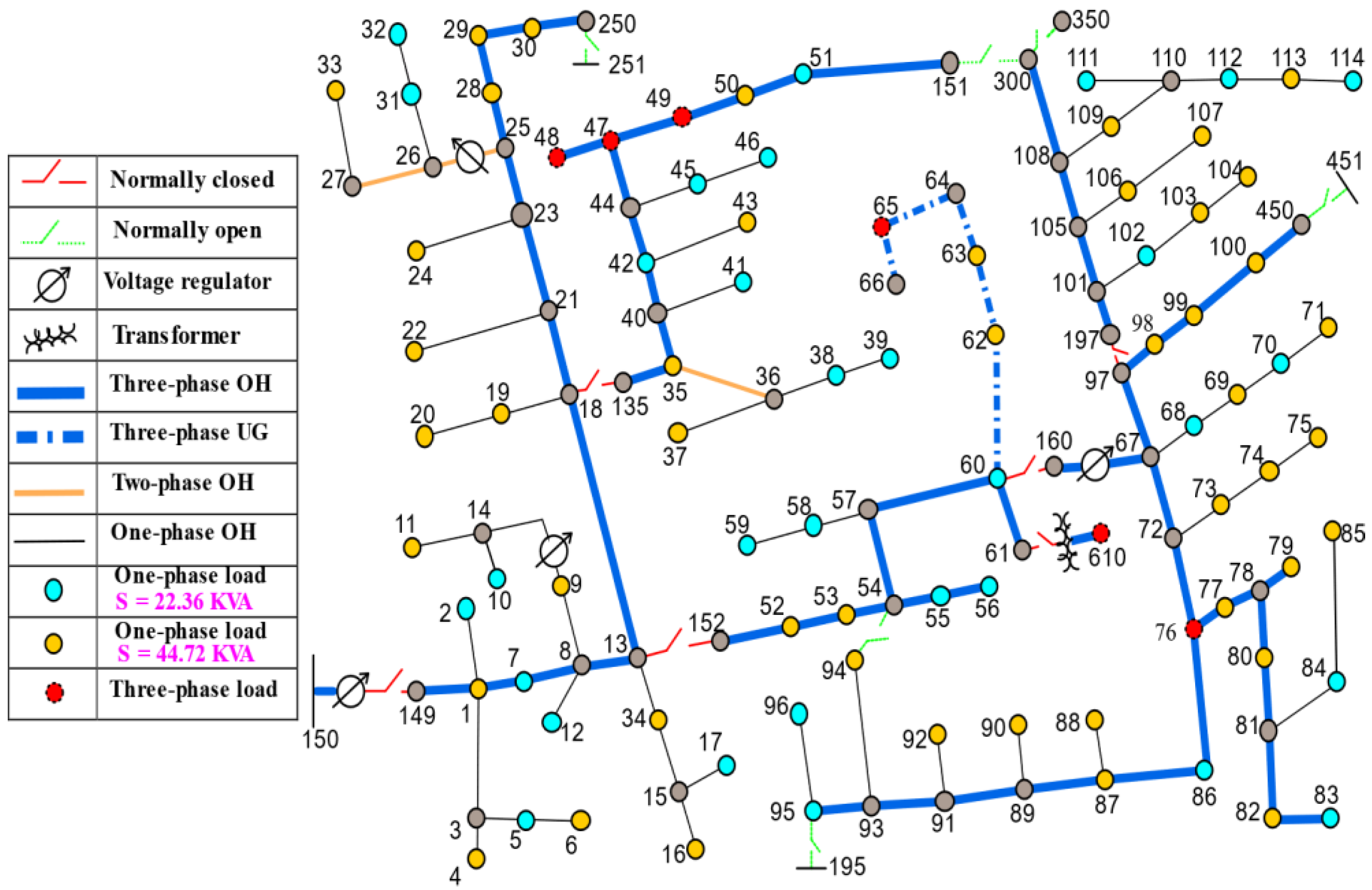
4.1. Test System

The distribution system under study, which is shown in Figure 12, consists of 123 buses and operates at a nominal voltage of 4.16 kV [37]. The main feeder radially emanates from the substation and is fed by a three-phase transformer bank of 5 MVA at the substation. The test bed system is modified to connect the FCS to the primary main feeder via a three-phase distribution transformer which was included in the system by replacing the three-phase loads shown in Figure 12. The IEEE 123-node system is modelled using the MATrix LABoratory (MATALB) software [38], and simulated in the Open Distribution System Simulator (OpenDSS) [39], using the Component Object Model (COM) interface. Two different charging methods, namely, uncontrolled charging and smart charging, are performed to evaluate their impact on voltage fluctuation and light flicker, as outlined in Algorithm 1. In each charging method, five case studies are considered whereby, in each case, a subset of all BPEVs in the system needs to charge from the FCS which is connected to the primary main feeder using a three-phase distribution transformer rated. In each case, the subset penetration is increased from 10% to 50%, by 10%.
Algorithm 1. Estimation and Assessment of Smart and Uncontrolled Charging Profiles.
1: Start
2: Input:
Number of EVs in the system
Share of Evs with respect of vehicles in the system
Number of residential houses in the system
Number of vehicles per house
Share of BPEVs charges from fcs
Share of BPEVs with small battery capacity that charge from FCS
Share of BPEVs with medium battery capacity that charge from FCS
Share of BPEVs with large battery capacity that charge from FCS
Probability distribution of vehicle arrival rate and time at the FCS
Probability distribution of battery state-of-charge at the start of charging event at an fcs.
Probability distribution of length of time with BPEV drawing power from an FCS
Probability distribution of battery state-of-charge at end of charging from an FCS
The maximum output power per each port of the FCS
The upper limits of premium, regular, and economic charging power
The lower limits of premium, regular, and economic charging power
FCS efficiency
3: For each BPEV do
4:      Generate a sample representing BPEV arrival rate and time
5: Determine vehicle’s battery capacity
6: Generate a sample representing BPEV state-of-charge at the start of charging
7: Generate a sample representing BPEV state-of-charge at the end of charging
8:      If the port is not available and state of charge   at   the   arrival   time > 10 %
9:      PBEV may or may not wait until the port becomes available, based on a random
    number uniformly distribution
10:      else
11:      BPEV will wait until the port becomes available
12:      End If
13:      If smart charging is selected
14:        Determine the charging power, premium, regular, or economic
15:        Consider the corresponding upper and lower limits
16: Determine the required state-of-charge accordingly
17:        Determine the departure time and then the charging duration is estimated
18: End If
19: Affix the estimated duration to the daily demand profile of smart charging starting from the hour in which arrival time was estimated
20:      If uncontrolled charging is selected
21:        Utilize the maximum charging power
22:        Determine the required state-of-charge accordingly
23:        Determine the departure time and then the charging duration is estimated
24: End If
25: Affix the estimated duration to the daily demand profile of uncontrolled charging starting from the hour in which arrival time was estimated
26:   End For
27: Affix the generated daily profile to the IEEE 123 test system to the node in which FCS is connected
28: Run the power flow analysis and report the voltages at all buses for 24 h
29: Assess the flicker at point-of-common coupling in which the FCS is installed
30: End

4.2. Charging Methods

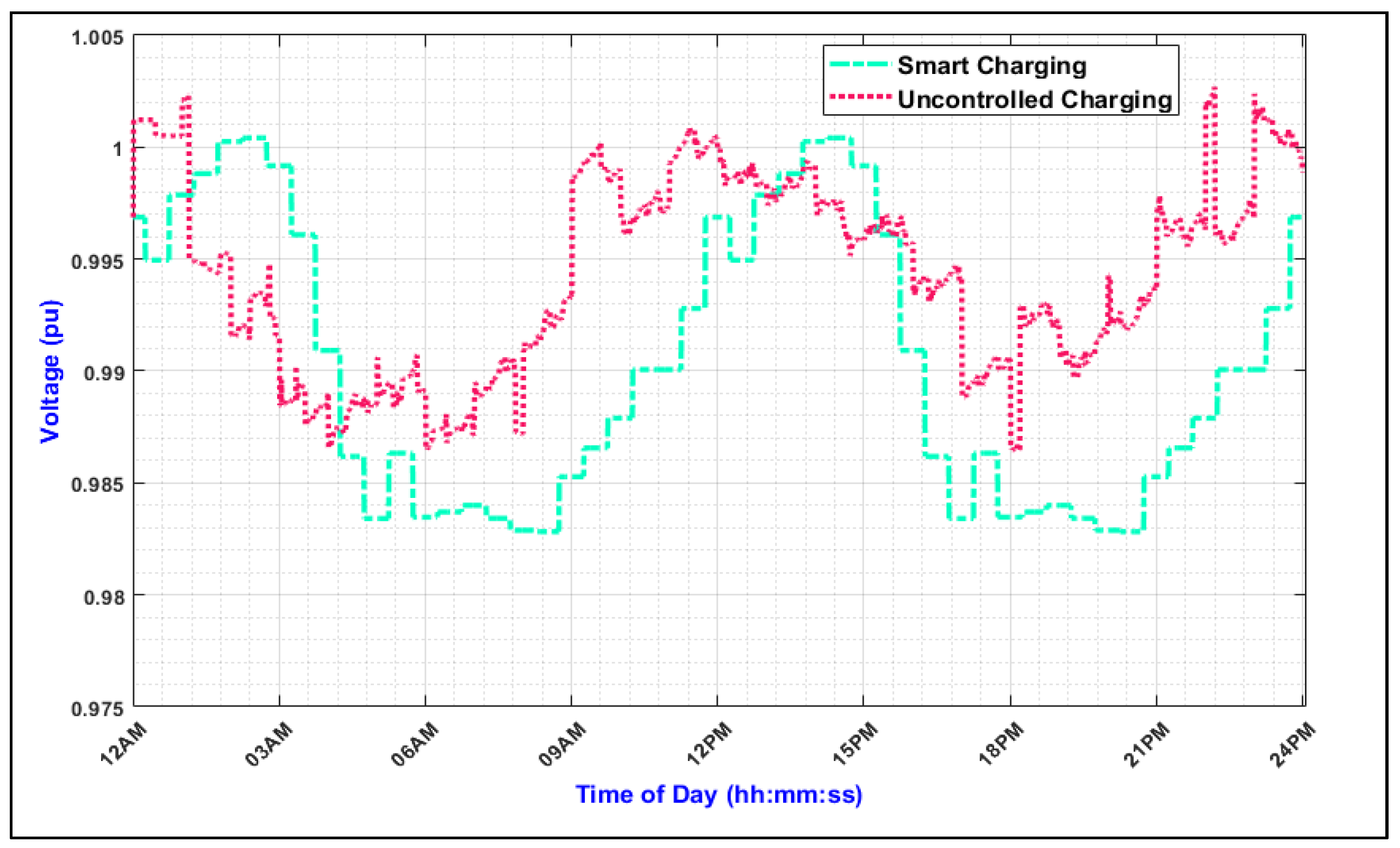
4.2.1. Uncontrolled Charging

In this case, when vehicles arrive at the FCS, they charge using the maximum rated power of the charger. Therefore, there is no control on the output power of the charger. A daily charging profile is generated accordingly. This profile represents the demand of the FCS on the distribution system under study. Consequently, the flicker severity is assessed as in Equation (51).

4.2.2. Smart Charging

In this case, a control is applied to the output power of the FCS. Therefore, three smart (controlled) charging powers are available at the FCS, namely, premium, regular, and economic power. In this case, constraint (52) is imposed to generate the daily charging profile generated, as explained previously in Section 2. The generated profile, as per the proposed smart charging method, represents the demand of the FCS on the system under study. This profile is affixed to the PCC, at node 48 in Figure 12, to which the FCS is connected, and thus utilized to estimate the flicker severity. The flicker severity in (51) is affected by the number of voltage dips per minute ( Ω ). The dips per minute is a function of the status of the chargers. When a fast charger is activated (ON), it charges the vehicle with an output power of β F C S kw. When the charger is deactivated (OFF), the output power goes to zero kw. In the ON/OFF status of the charger, the voltage at the PCC dips and deviates ( Δ U ). The dips per minute is affected by the penetration of BPEVs charging from the FCS. When the penetration is increased, the dips per minute is increased, and vice versa. Therefore, different FCS penetrations (10%, 20%, 30%, 40%, and 50%) have been considered. In each penetration, the dips per minute is determined and the flicker severity in Equation (51) is calculated accordingly. The penetration of vehicles charging from the FCS,   Λ F C S , is a function of the total BPEVs in the system, N B P E V , which in turn is a function of the number of houses, i.e., 750 houses, and two vehicles per house [7]. Vehicles, which charge from the FCS, arrive there according to the distribution shown in Figure 4. The highest rate of arrival at the FCS is >7%, as presented in Figure 4, occurs at 4:00 p.m. This means that more than 7% of all vehicles charge from the FCS at 4:00 p.m. Given the arrival rate at the FCS at 4:00 p.m., the penetration of vehicles charging from the FCS, and the number of BPEVs in the system, the dips per minute are determined accordingly, as shown in Table 3. Where using the FCS contributes to light flicker, it mostly occurs at the hour that has the highest arrival rate (at 4:00 p.m.); thus, at this hour, the flicker severity index is at its highest value. If smart charging is able to mitigate flicker severity at that hour (4:00 p.m.), it implies that the flicker severity during the rest of the day is reduced by the proposed smart charging (according to the arrival rates and times in Figure 4). Therefore, the FCS flicker severity at 4:00 p.m. is evaluated by both the proposed smart charging and the uncontrolled charging methods. The results of the evaluation are presented below.

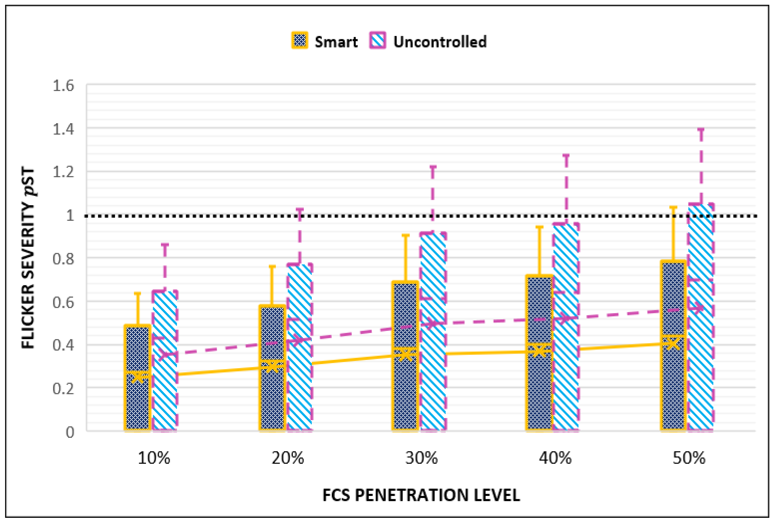
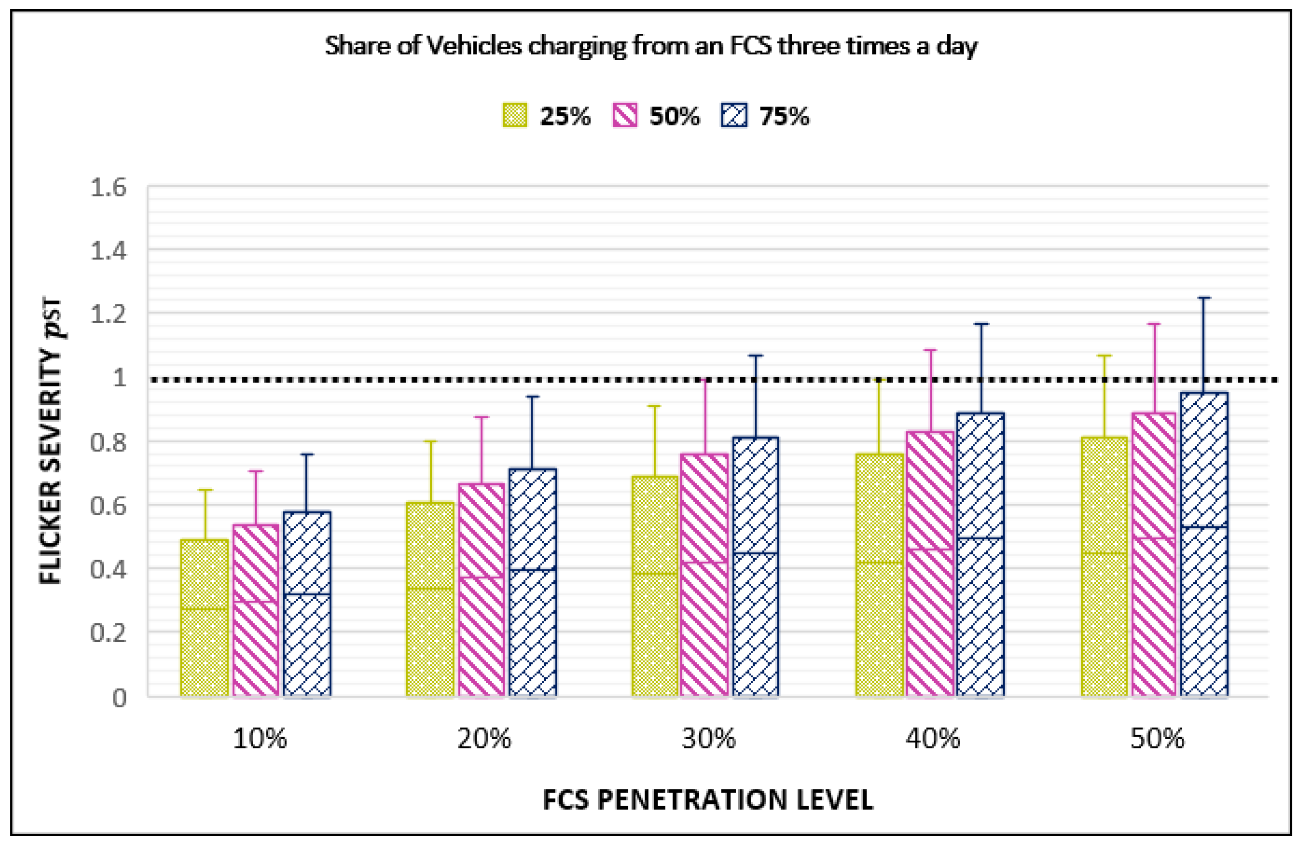
4.3. Effect of Uncontrolled and Smart Charging on Flicker Seversity

Figure 13 shows the daily charging demand on the FCS and encompasses three groups of vehicles, according to the used charging power. These groups charge from the FCS using premium, regular, and economic charging power (as shown in the y-axis titles). Each horizontal bar in Figure 13 represents the charging duration of a vehicle using that charging power mentioned in the y-axis. The total number of horizontal bars show the total number of vehicles that charge from the FCS on that day. In the case of uncontrolled charging power, all vehicles in Figure 13 charge using the same charging power ( β u ). When the penetration of vehicles that charge from the FCS is increased, the number of horizontal bars, as shown in Figure 13, is increased which, in turn, increases the daily voltage dips because of the on/off status of the chargers. Figure 14 depicts minimum and maximum line-to-neutral voltages experienced during the day by each node in the system under study. Figure 15 depicts the comparison of flicker severity for both methods of charging. The x-axis shows different penetration levels that represent the increased demand of vehicles on the FCS at the same hour of the day, i.e., at 4:00 p.m. The flicker severity values are depicted in the y-axis in Figure 15. A light flicker is observed if the flicker severity exceeds 1. It is noted from Figure 15 that as the penetration level is increased, the flicker index increases. When the FCS charges vehicles by the uncontrolled charging method, the FCS violates the flicker tolerance, especially when the demand on its service is increased by 20% and beyond. In contrast, the flicker limit is not violated when vehicles charge from the FCS as per the proposed smart charging approach, even when the penetration on the FCS is increased by 50%.
Therefore, the proposed smart charging approach clearly shows that it is effective not only in mitigating voltage fluctuations and light flicker, but also in reducing the flicker severity even when the FCS voltage dip per minute is increased by five times. Figure 16 shows the voltage in per unit measured at primary side of distribution transformers at bus 48, in which FCS is connected.

4.4. Effect of Full Battery Charging on Flicker Severity

In the previous section, the reported results assume that vehicles start their first trip from home with different SOCs, as shown in Figure 5. Most of these vehicles start the trip with almost fully charged batteries (i.e., >90%). The reported results assume that vehicles are charged at night, so that, in the morning, they start their trip with different SOCs, as shown in Figure 5. Before they arrive home, a share of these vehicles requires a charge from the FCS, according to Figure 3, and arrive at the FCS with different SOCs, distributed as in Figure 8, at different arrival rates, as shown in Figure 4. There is no direct effect of full battery charging on the flicker severity index. Equation (48) shows the factors that impact flicker severity, which is affected mainly by dips per unit time. The dip is a function of the on/off states of the fast charger. When penetration of BPEVs that use the FCS is increased, the dips per unit time is also increased. It is important to consider what would motivate a customer with a home charger, whose battery capacity is large and whose daily round trip to/from home is within the battery driving range, to pay for charging via a fast charger. The willingness to pay for charging is driven by the value of charging time or the opportune cost of charging which, in turn, varies according to the segment of the market and consumers [40]. For personal use and privately-owned EVs, most charging events are performed by home or work chargers where the vehicle is parked for long periods of time. During this time, the value of charging time is low, thus home or work chargers, which are characterized as slow chargers, are convenient. However, for shared privately-owned ride hailing or commercial automated ride-hailing EVs, the value of charge time is high, especially for on-shift charging [40]. EVs in this sector drive 29% more daily miles, require two times more charging power, and utilize three times more fast chargers than personal-use vehicles, as reported in [41]. As free-floating car-sharing is adopted, the dependency on the FCS is increased to reduce downtime due to charging, thus the dips per unit time is expected to increase because of increasing FCS daily usage.

4.5. Effect of Flicker Enverlope

This section investigates flicker severity when the daily usage of the FCS is increased according to the proposed smart charging method. The results of flicker severity are depicted in Figure 17. Although the penetration of vehicles in Figure 17 that charge from an FCS is similar to their penetration in Figure 15, they are different in that the share of vehicles (25%, 50%, and 75%) per penetration level in Figure 17 charges from the FCS three times a day, to imitate the charging pattern of shared EVs. Therefore, according to the arrival rate presented in Figure 4, the highest rate of vehicles arriving at the FCS is at 4:00 p.m. The dips per hour in Figure 17 is three times more than that in Figure 15. The aim is to show the ability of the proposed smart charging method to reduce the flicker level if daily usage of the FCS per vehicle is increased.
The results in Figure 17 show that the proposed smart charging method can mitigate the flicker level, even if the penetration of vehicles that charge from the FCS is increased up to between 20% and 75% and these vehicles charge from an FCS three times a day. When the share of vehicles that charge from an FCS three times a day is reduced to 25%, the proposed smart charging is able to reduce the flicker level, even if the penetration of vehicles charging from an FCS is increased to 40%. Beyond this penetration and daily utilization rates, the flicker limit is exceeded.

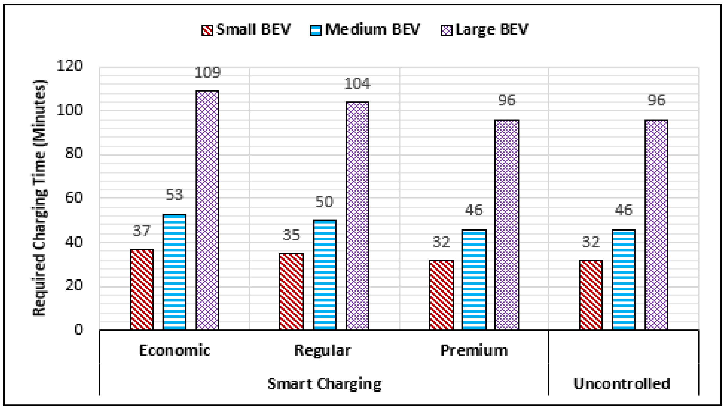
4.6. Effect of Smart Charging on Charging Duration

Figure 18 presents the required charging time to charge vehicles with different battery capacities via a 50 kw fast charger. The charging duration for each vehicle is calculated when its battery SOC is changed from 20% to 80% using the uncontrolled and the proposed smart charging methods. As the output power of the charger is increased, the time it takes to charge the vehicle’s battery is decreased. The uncontrolled charging provides the highest output power; thus, it requires less time to charge the battery SOC from 20% to 80% in comparison to the economic and regular charging methods, as depicted in Figure 18. However, when the station encompasses multiple fast chargers and their operations are uncontrolled, a voltage fluctuation may occur which, in turn, may cause the limit of light flicker to be exceeded. In contrast, the light flicker limit will not be violated when the proposed smart charging is utilized. However, the time it takes for vehicles to charge their batteries with the same amount of energy using smart charging (economic or regular) is more than what it takes to charge by the uncontrolled charging. Therefore, in order to make customers adopt the smart charging method, the FCS operator/investor must offer a compromise solution that meets the regulation of the service provider and the needs of customers.

4.7. Comparative Study

A comparison study is conducted between the proposed method and the other existing studies in the literature. The comparison is conducted according to the reported flicker value. Table 4 presents a comparison of flicker values as reported in the previous work as well as in the current study. Unlike uncontrolled charging, the proposed smart charging method is able to reduce the light flicker and enables an FCS to increase its rate of utilization without exceeding the standard limit of flicker. It is to be noted that the flicker values shown in Table 4 represent the short-term flicker severity index.

5. Conclusions

A novel smart charging approach is proposed in this work to mitigate the impact of FCSs on voltage fluctuation and light flicker. The proposed charging method assumes that the same port of a fast charger can provide three different levels of charging powers, namely, economic, regular, and premium. Selection of the charging power is determined by the customer, but their charging rates are defined by the FCS operator/investor and can be changed within the day according to different variables, such as system peak, FCS demand, and the local level of produced renewable energy. The objective and constraints related to smart charging are included in this study. The effect of the proposed charging on charging duration as well as the effect of full charging of batteries is analyzed. Two case studies were conducted to evaluate the impact of the proposed smart charging method, as well as uncontrolled charging, on voltage fluctuation and light flicker. The results reveal that integrating the FCS has an adverse impact on the voltage fluctuations that lead to light flicker. The impact is a function of different parameters such as the rated power of the charger, the number of chargers in the station, and share of vehicle charges from the FCS. When the uncontrolled charging method is applied, the flicker limit is exceeded when the demand on the FCS station is increased by 20%. In contrast, the proposed smart charging can mitigate voltage fluctuation and light flicker even when the penetration on the FCS is increased by 50%. Reducing the system peak was not considered in this study and it is a benefit for the system operator. The proposed smart charging method can be formulated to consider the system peak and the time-of-use price in its constraints, which is open the door for a future work.

Funding

This research received no external funding.

Institutional Review Board Statement

Not applicable.

Informed Consent Statement

Not applicable.

Acknowledgments

Sami M. Alshareef would like to acknowledge the funding support received from Jouf University, Saudi Arabia, to conduct this study.

Conflicts of Interest

The author declares no conflict of interest.

Nomenclature

N B P E V Number of BPEV in the system
x p e n Share of electric vehicles with respect to the total number of vehicles in the system
n h o u s e Number of residential houses in the system, 750 houses
n c a r Number of vehicles per house, 2 vehicles/house
μ v Battery capacity of vehicle v , kwh
μ s Capacity of small battery, k w h
μ m Capacity of medium battery, k w h
μ l Capacity of large battery, k w h
V s A set of PEVS with small battery capacity
V m A set of PEVS with medium battery capacity
V l A set of PEVS with large battery capacity
V H o m e A set of PEVS uses the home chargers
V F C S A set of PEVS uses the FCS
k w h F C S Energy required for vehicle v from FCS, kwh
L F C S Length of time with vehicle v connected to the fast charger, minute
η F C S Efficiency of the fast charger, %
ϑ Factor to convert hour into minutes
β Maximum charging power per port, kw
β F C S Output power of fast-charging station, kw
β u Uncontrolled charging power, kw
β p Premium charging power, kw
β r Regular charging power, kw
β e Economic charging power, kw
N t p Number of PEV that charging using premium charging power at time t
N t r Number of PEV that charging using regular charging power at time t
N t e Number of PEV that charging using economic charging power at time t
p ¯ Factor to set the upper limits of premium charging power, %
p ¯ Factor to set the lower limits of premium charging power, %
r ¯ Factor to set the upper limits of regular charging power, %
r ¯ Factor to set the lower limits of regular charging power, %
e ¯ Factor to set the upper limits of economic charging power, %
e ¯ Factor to set the lower limits of economic charging power, %
K Capacity of the FCS, kw
p o r t s Number of ports in the fast-charging station
η S Share of BPEV with small battery capacity s charges at the FCS at time t , p . u .
η m Share of BPEV with medium battery capacity m charges at the FCS at time t , p . u .
η l Share of BPEV with large battery capacity l charges at the FCS at time t , p . u .
α t , b c , p d e Share of BPEV that have battery capacity b c charged using premium charging power at FCS at time t and required departure time of d e , p . u .
α t , b c , r d e Share of BPEV that have battery capacity b c charged using regular charging power at time t and required departure time of d e , p . u .
α t , b c , e d e Share of BPEV that have battery capacity b c charged using economic charging power at time t and required departure time of d e , p . u .
Λ F C S Share of BPEV that uses FCS, p . u .
V F C S , p v A set of BPEV uses the premium charging power
V F C S , r v A set of BPEV uses the regular charging power
V F C S , e v A set of BPEV uses the economic charging power
V F C S s Number of PEV with small battery capacity uses the FCS
V F C S m Number of PEV with medium battery capacity uses the FCS
V F C S l Number of PEV with large battery capacity uses the FCS
s o c t v State-of-charge of vehicle v at time t
s o c t 1 v State-of-charge of vehicle v at time t 1
s o c r e q Minimum energy required from the FCS
s o c d e s v Desired state-of-charge at the departure time t ν d e of vehicle v , %
s o c m a x v Maximum state-of-charge at the departure time t ν d e of vehicle v , %
t ν d e Departure time of vehicle v
Γ Relative voltage changes caused by FCS at point-of-common, %
Δ U Voltage variation at point-of-common coupling, k V
U p c c Nominal voltage at point-of-common, k V
Δ S Apparent power variation at point-of-common coupling, k V A
Δ P Active power load change at point-of-common coupling, k w
Δ Q Reactive power load change at point-of-common coupling, k V A r
Δ Ι Current load change at point-of-common coupling, A m p
θ Network impedance angle, degree
χ p c c Network reactance at point-of-common, ohms
r p c c Network resistance at point-of-common, ohms
Flicker time represents the flicker impression of a single voltage change, second
φ Factor represents the waveform shape of voltage fluctuation, rectangular change
Factor to comply with the flicker curve
γ Coefficient to describe the source of disturbance
ξ Summation of all flicker times, minute
Ω Number of voltage dips per minute
p p c c s t Limit of short-term flicker severity

References

  1. Gao, Z.; Mao, D.; Wang, J. Distribution grid response monitor. IET Gener. Transm. Distrib. 2019, 13, 4374–4381. [Google Scholar] [CrossRef]
  2. Dominion Energy. 2017 Blue Book; Dominion Energy Virginia and Dominion Energy: Elizabeth City, NC, USA, 2019. [Google Scholar]
  3. Duke Energy Midwest Duke Energy Midwest Transmission Systems Facility Connection Requirements. Available online: https://dms.psc.sc.gov/Attachments/Matter/af2591fc-cdb8-af85-a7faf2d347bd0c65 (accessed on 11 December 2019).
  4. Engineering Recommendation P28 Voltage Fluctuations and the Connection of Disturbing Equipment to Transmission Systems and Distribution Networks in the United Kingdom. Available online: https://www.nienetworks.co.uk/documents/d-code/ena_erec_p28_issue-2_(2019).aspx/ (accessed on 4 May 2019).
  5. Alhazmi, Y.A.; Salama, M.M.A. Economical staging plan for implementing electric vehicle charging stations. Sustain. Energy Grids Netw. 2017, 10, 12–25. [Google Scholar] [CrossRef]
  6. Sharma, I.; Canizares, C.; Bhattacharya, K. Smart charging of PEVs penetrating into residential distribution systems. IEEE Trans. Smart Grid 2014, 5, 1196–1209. [Google Scholar] [CrossRef]
  7. Humayd, A.S.B.; Bhattacharya, K. Design of optimal incentives for smart charging considering utility-customer interactions and distribution systems impact. IEEE Trans. Smart Grid 2017, 10, 1521–1531. [Google Scholar] [CrossRef]
  8. Hafez, O.; Bhattacharya, K. Integrating EV charging stations as smart loads for demand response provisions in distribution systems. IEEE Trans. Smart Grid 2016, 9, 1096–1106. [Google Scholar] [CrossRef]
  9. Moghaddam, Z.; Habibi, D. Smart Charging Strategy for Electric Vehicle Charging Stations. IEEE Trans. Transp. Electrif. 2018, 4, 13. [Google Scholar] [CrossRef]
  10. van der Kam, M.; van Sark, W. Smart charging of electric vehicles with photovoltaic power and vehicle-to-grid technology in a microgrid; a case study. Appl. Energy 2015, 152, 20–30. [Google Scholar] [CrossRef] [Green Version]
  11. Humayd, A.S.B.; Lami, B.; Bhattacharya, K. The effect of PEV uncontrolled and smart charging on distribution system planning. In Proceedings of the 2016 IEEE Electrical Power and Energy Conference (EPEC), Ottawa, ON, Canada, 12–14 October 2016; IEEE: New York City, NY, USA, 2016; pp. 1–6. [Google Scholar]
  12. Almutairi, A.; Salama, M.M.A. Assessment and Enhancement Frameworks for System Reliability Performance Using Different PEV Charging Models. IEEE Trans. Sustain. Energy 2018, 9, 1969–1984. [Google Scholar] [CrossRef]
  13. Alshareef, S.M.; Morsi, W.G. Impact of fast charging stations on the voltage flicker in the electric power distribution systems. In Proceedings of the 2017 IEEE Electrical Power and Energy Conference (EPEC), Saskatoon, SK, Canada, 22–25 October 2017; pp. 1–6. [Google Scholar]
  14. Diaz, C.; Ruiz, F.; Patino, D. Smart charge of an electric vehicles station: A model predictive control approach. In Proceedings of the 2018 IEEE Conference on Control Technology and Applications (CCTA), Copenhagen, Denmark, 21–24 August 2018; IEEE: New York City, NY, USA, 2018; pp. 54–59. [Google Scholar]
  15. Marei, M.I.; El-Saadany, E.F.; Salama, M.M. Envelope tracking techniques for FlickerMitigation and Voltage regulation. IEEE Trans. Power Deliv. 2004, 19, 1854–1861. [Google Scholar] [CrossRef]
  16. Marei, M.I.; Salama, M.M.A. Advanced Techniques for Voltage Flicker Mitigation. In Proceedings of the 2006 IEEE International Power Electronics Congress, Puebla, Mexico, 16–18 October 2006; IEEE: New York City, NY, USA, 2006; pp. 1–5. [Google Scholar]
  17. Elnady, A.; Salama, M.M. Unified approach for mitigating voltage sag and voltage flicker using the DSTATCOM. IEEE Trans. Power Deliv. 2005, 20, 992–1000. [Google Scholar] [CrossRef]
  18. Perera, D.; Meegahapola, L.; Perera, S.; Ciufo, P. Characterisation of flicker emission and propagation in distribution networks with bi-directional power flows. Renew. Energy 2014, 63, 172–180. [Google Scholar] [CrossRef] [Green Version]
  19. Eghtedarpour, N.; Farjah, E.; Khayatian, A. Effective Voltage Flicker Calculation Based on Multiresolution S-Transform. IEEE Trans. Power Deliv. 2012, 27, 521–530. [Google Scholar] [CrossRef]
  20. Robert, A.; Couvreur, M. Recent experience of connection of big arc furnaces with reference to flicker level. In Proceedings of the International Conference on Large High Voltage Electric Systems, Interlaken, Switzerland, 24–29 July 1994; pp. 36–305. [Google Scholar]
  21. Arlt, D.; Stark, M.; Eberlein, C. Examples of international flicker requirements in high voltage networks and real world measurements. In Proceedings of the 2007 9th International Conference on Electrical Power Quality and Utilisation, Barcelona, Spain, 9–10 October 2007; IEEE: Barcelona, Spain, 2007; pp. 1–4. [Google Scholar]
  22. Perera, S.; Robinson, D.; Elphick, S.; Geddey, D.; Browne, N.; Smith, V.; Gosbell, V. Synchronized flicker measurement for flicker transfer evaluation in power systems. IEEE Trans. Power Deliv. 2006, 21, 1477–1482. [Google Scholar] [CrossRef]
  23. Irena Innovation Outlook Smart Charging for Electric Vehicles. Available online: https://www.irena.org/publications/2019/May/Innovation-Outlook-Smart-Charging/ (accessed on 5 January 2019).
  24. IRENA Innovation Landscape Brief: Electric-Vehicle Smart Charging. Available online: https://irena.org/-/media/Files/IRENA/Agency/Publication/2019/Sep/IRENA_EV_smart_charging_2019.pdf?la=en&hash=E77FAB7422226D29931E8469698C709EFC13EDB2 (accessed on 5 January 2019).
  25. Alshareef, S.M.; Morsi, W.G. Probabilistic Modeling of Plug-in Electric Vehicles Charging from Fast Charging Stations. In Proceedings of the 2019 IEEE Electrical Power and Energy Conference (EPEC), Montreal, QC, Canada, 16–18 October 2019; IEEE: Montréal, QU, Canada, 2019; pp. 1–6. [Google Scholar]
  26. Axsen, J.; Goldberg, S.; Bailey, J.; Kamiya, G.; Langman, B.; Cairns, J.; Wolinetz, M.; Miele, A. Electrifying Vehicles: Insights from the Canadian Plug-in Electric Vehicle Study. Simon Fraser University, Vancouver, Canada. Available online: https://sustainabletransport.ca/the-canadian-plug-in-electric-vehicle-study-cpevs/ (accessed on 12 March 2019).
  27. Duvall, M.; Knipping, E.; Alexander, M.; Tonachel, L.; Clark, C. Environmental assessment of plug-in hybrid electric vehicles, Volume 1: Nationwide greenhouse gas emissions. Electr. Power Res. Inst. Palo Alto CA 2007, 1015325. Available online: https://www.energy.gov/sites/prod/files/oeprod/DocumentsandMedia/EPRI-NRDC_PHEV_GHG_report.pdf (accessed on 4 May 2020).
  28. evCloud | FleetCarma. Available online: https://www.fleetcarma.com/evCloud (accessed on 19 December 2018).
  29. Gjelaj, M.; Træholt, C.; Hashemi, S.; Andersen, P.B. DC Fast-charging stations for EVs controlled by a local battery storage in low voltage grids. In Proceedings of the PowerTech, 2017 IEEE Manchester, Manchester, UK, 18–22 June 2017; IEEE: Manchester, UK, 2017; pp. 1–6. [Google Scholar]
  30. Francfort, J.; Brion Bennett, R. Plug-in Electric Vehicle and Infrastructure Analysis. Available online: https://inldigitallibrary.inl.gov/sites/sti/sti/6799570.pdf (accessed on 13 October 2019).
  31. Vehicle Technologies Office Avta: Arra ev Project Chevrolet Volt Data Summary Reports. Available online: https://www.energy.gov/eere/vehicles/downloads/avta-arra-ev-project-chevrolet-volt-data-summary-reports (accessed on 7 July 2020).
  32. Petro-Canada Reveals $0.33 per Minute EV Charging Cost in Ontario. Available online: https://mobilesyrup.com/2020/01/22/petro-canada-33-cents-per-minute-ev-cost/ (accessed on 11 September 2020).
  33. IEC/TR 61000-3-7; Electromagnetic Compatibility (EMC). Part 3: Limits—Section 7: Assessment of Emission Limits for Fluctuating Loads in MV and HV Power Systems. International Electrotechnical Commission: Geneva, Switzerland, 1996; Volume 61, pp. 1–10.
  34. IEC 61000-3-3:2013; Electromagnetic Compatibility (EMC). Part 3-3, Limits–Limitation of Voltage Changes, Voltage Fluctuations and Flicker in Public Low-Voltage Supply Systems, for Equipment with Rated Current≤ 16 A per Phase and Not Subject to Conditional Connection. International Electrotechnical Commission: Geneva, Switzerland, 2013; pp. 61000–61003.
  35. Baggini, A. Handbook of Power Quality; John Wiley & Sons: Hoboken, NJ, USA, 2008; ISBN 0-470-75423-0. [Google Scholar]
  36. IEEE Std 1453-2015; IEEE Recommended Practice–Adoption of IEC 61000-4-15:2010, Electromagnetic Compatibility (EMC)–Testing and Measurement Techniques–Flickermeter–Functional and Design Specifications. IEEE: New York City, NY, USA, 2019. Available online: https://ieeexplore.ieee.org/document/6053977 (accessed on 17 February 2022).
  37. IEEE PES AMPS DSAS Test Feeder Working Group Resources. PES Test Feeder. Available online: http://sites.ieee.org/pes-testfeeders/resources/ (accessed on 11 March 2019).
  38. MATLAB Release 2020b; The MathWorks, Inc.: Natick, MA, USA, 1992.
  39. EPRI, Smart Grid Resource Center. Simulation Tool—OpenDSS. Available online: https://smartgrid.epri.com/SimulationTool.aspx (accessed on 17 February 2022).
  40. Smart, J. Charging Infrastructure for Shared and Autonomous EVs. In Proceedings of the Future of Electric Vehicle Infrastructure in the U.S. Webinar, Online, 2 May 2019. [Google Scholar]
  41. Wood, E.; Rames, C.; Kontou, E.; Motoaki, Y.; Smart, J.; Zhou, Z. Analysis of Fast Charging Station Network for Electrified Ride-Hailing Services. In Proceedings of the SAE World Congress Experience, Detroit, MI, USA, 10–12 April 2018. SAE Technical Paper 2018-01-0667. [Google Scholar]
  42. Rosnan, T.D.; Murray, M.A. Voltage fluctuation monitoring in an ESB Transmission station. In Irish Colloquium on DSP & Control; University of Limerick: Dublin, Ireland, 1993. [Google Scholar]
  43. Brosnan, T.D.; Murray, M.A. Flicker Severity Measurements on an Electric Arc Furnace during Switched Changes in a Transmission Network. In Proceedings of the First International Conference on Power Quality, Paris, France, 15–18 October 1991. [Google Scholar]
  44. Arlt, D.; Eberlein, C. Network disturbances caused by Ultra High Power electric arc furnaces and possible reduction methods. In Proceedings of the Conference Electrical Power Quality and Utilisation, Cracow, Poland, 23–25 September 1997; pp. 23–25. [Google Scholar]
  45. d’études, C.; Arlt, D.; Papič, I. C4, C. international des grands réseaux électriques. In Review of Flicker Objectives for LV, MV, and HV Systems: Cigre/Cired; CIGRÉ: Paris, France, 2011; ISBN 978-2-85873-138-1. [Google Scholar]
Figure 1. Effect of voltage fluctuation on different stakeholders.
Energies 15 01746 g001
Figure 2. Comparison of smart charging and services provided to the grid [24].
Energies 15 01746 g002
Figure 3. Charging events by location [26].
Energies 15 01746 g003
Figure 4. Percentage of BPEVs arriving per hour at the fast charging station (arrival rate) [28].
Energies 15 01746 g004
Figure 5. Battery state of charge at end of charging from home charger prior to driving [30].
Energies 15 01746 g005
Figure 6. Nissan battery state of charge at the start of charging events [31].
Energies 15 01746 g006
Figure 7. Chevrolet battery state of charge at the start of charging events [31].
Energies 15 01746 g007
Figure 8. Average battery state of charge at the start of charging events at an FCS.
Energies 15 01746 g008
Figure 9. Distribution of length of time with a vehicle drawing power from an FCS per charging event [30].
Energies 15 01746 g009
Figure 10. Battery state of charge at end of charging from an FCS prior to driving.
Energies 15 01746 g010
Figure 11. Distribution of length of time with a vehicle connected to an FCS per charging event [30].
Energies 15 01746 g011
Figure 12. IEEE 123-node test feeder [37].
Energies 15 01746 g012
Figure 13. Daily demand per each charging power in an FCS.
Energies 15 01746 g013
Figure 14. Minimum and maximum voltage experienced by each primary node when FCSs are connected.
Energies 15 01746 g014
Figure 15. Comparison of flicker level for uncontrolled and proposed smart charging.
Energies 15 01746 g015
Figure 16. Voltage Waveform Measured at PCC at Node 48 When FCSs are Connected.
Energies 15 01746 g016
Figure 17. Flicker level when the penetration on the proposed smart charging increases.
Energies 15 01746 g017
Figure 18. Charging Duration to Increase Battery SOC from 20% to 80% using the smart and uncontrolled charging.
Energies 15 01746 g018
Table 1. Comparison of the previous work and the proposed method according to charging type and effect on light flicker.
ReferenceCharging PowerCharging TypeFlicker
SlowFastUncontrolledSmartAnalysisMitigation
[7,9,10,11]××××
[12]×××
[13]××××
[14]×××
[8]×××
[15,16,17]××××
[18,19,20,21,22]×××××
[6]××××
Proposed Smart Charging×
✓: Considered, ×: Not considered.
Table 2. Impact of charging method and type [23].
Slow ChargingFast Charging
UncontrolledSmartUncontrolledwith BatterySmart
Electricity demand+++++
Peak demand+++++++
Distribution grids+++++++
Light flicker×××
×: Not exceeding the limit the limit, ✓: Exceeding the limit, +: Affected, ++: More affected.
Table 3. Number of PBEVs Charging via Fast Charging Station.
Penetration
Level
(Increase of Λ F C S )
Number of PBEVs
in the System
( N B P E V )
Number of PBEVs Using the
FCS ( Λ F C S )
Dips per Minute
( Ω )
in 24 Hoursat 4:00 p.m.
10%1505140.14
20%30010280.28
30%450153120.42
40%600204160.56
50%750255200.7
Table 4. Comparison of the previous work and the proposed method according to flicker level.
ReferenceReported Flicker Value
Previous work[21]2
[20]1.7
[42]1.05
[43]1.4
[44]1.26
[22]2.78
[45]2.6
Current studyUncontrolled FCS, at 10% up to 40% of FCS utilization rate0.9–1.3
FCS with smart charging, at 10% up to 40% of FCS utilization rate0.6–0.9
Publisher’s Note: MDPI stays neutral with regard to jurisdictional claims in published maps and institutional affiliations.

