
Framework for Mapping and Optimizing the Solar Rooftop Potential of Buildings in Urban Systems

 , , ,
, , ,  and
and
Abstract
:1. Introduction
- Developing an advanced image processing method to consider unusual shapes of building roofs, roofs with obstacles, and roofs with different heights.
- Using the search space optimization method to deal with the non-linear problem with sensitive constraints, such as the number and location of PV panels and irregular roof dimensions, in addition to the main control variables: tilt and azimuth angles.
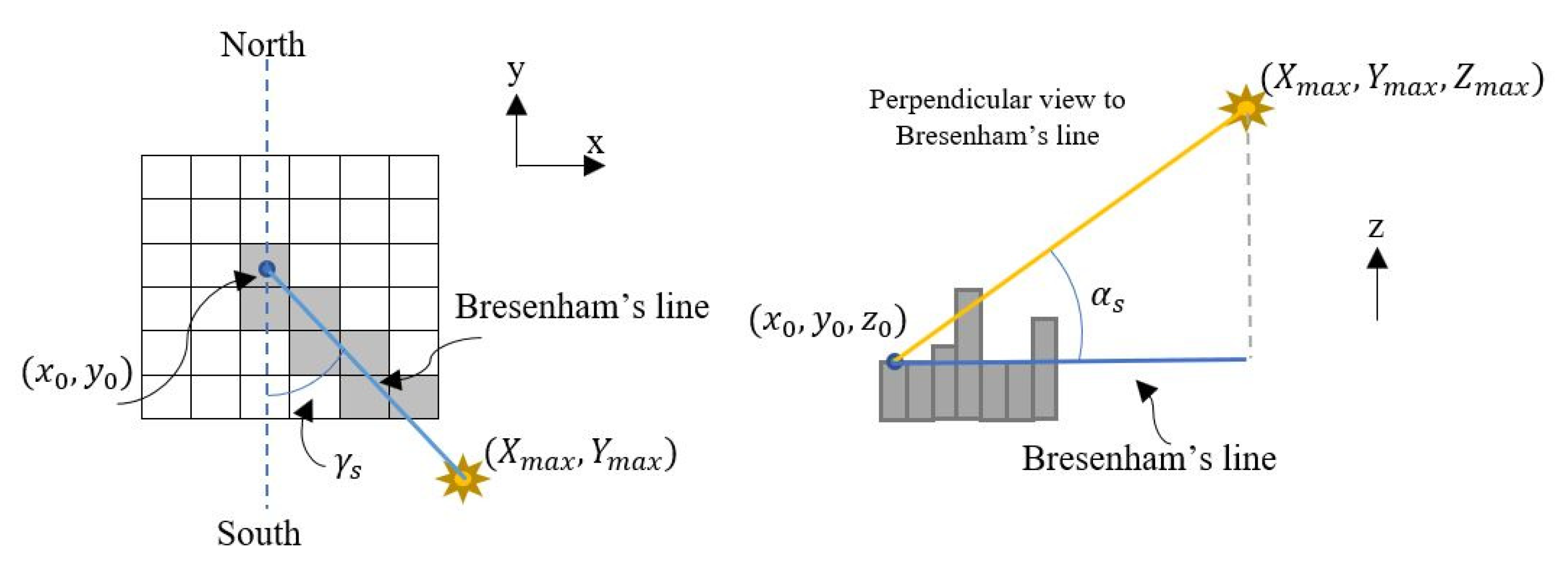
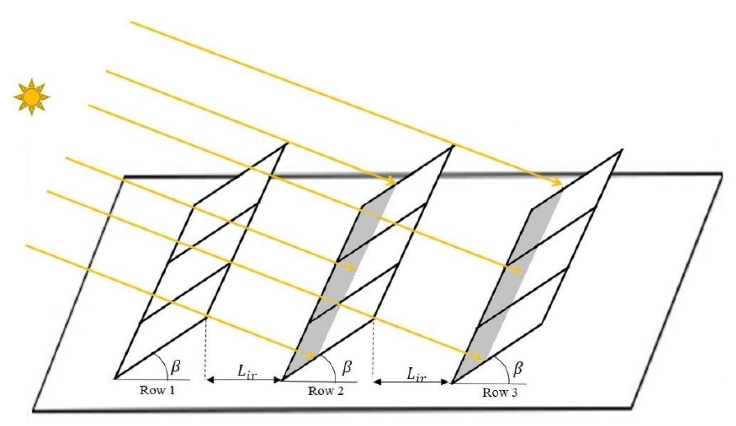
- Considering two types of shading impact: the mutual shading of the adjacent panels and the shading of surrounding objects such as higher roofs, parapets, trees, chimneys, large external HVAC systems, and neighbor buildings.
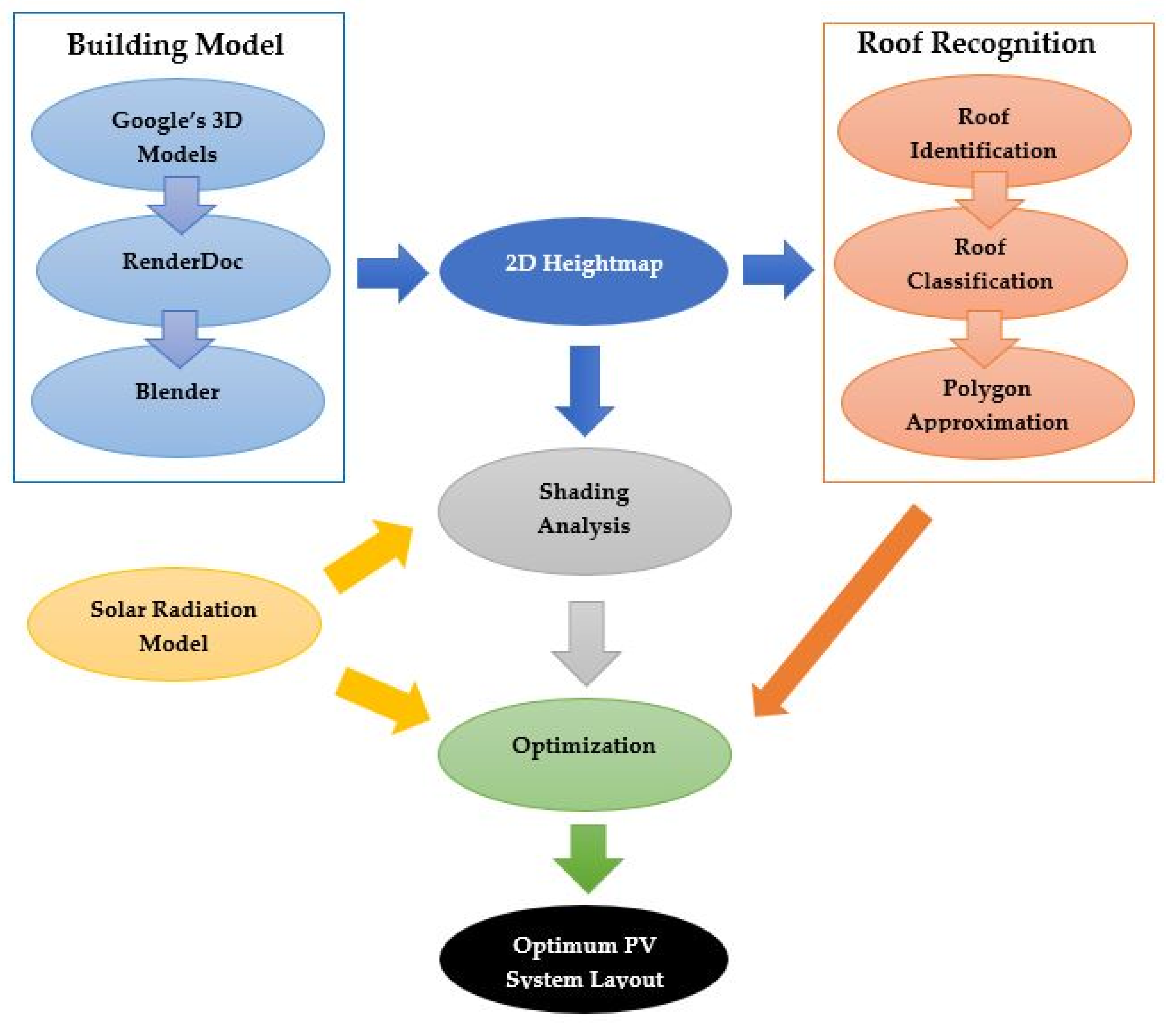
2. Materials and Methods
2.1. Building Models
2.2. Rooftop Recognition Using Computer Vision
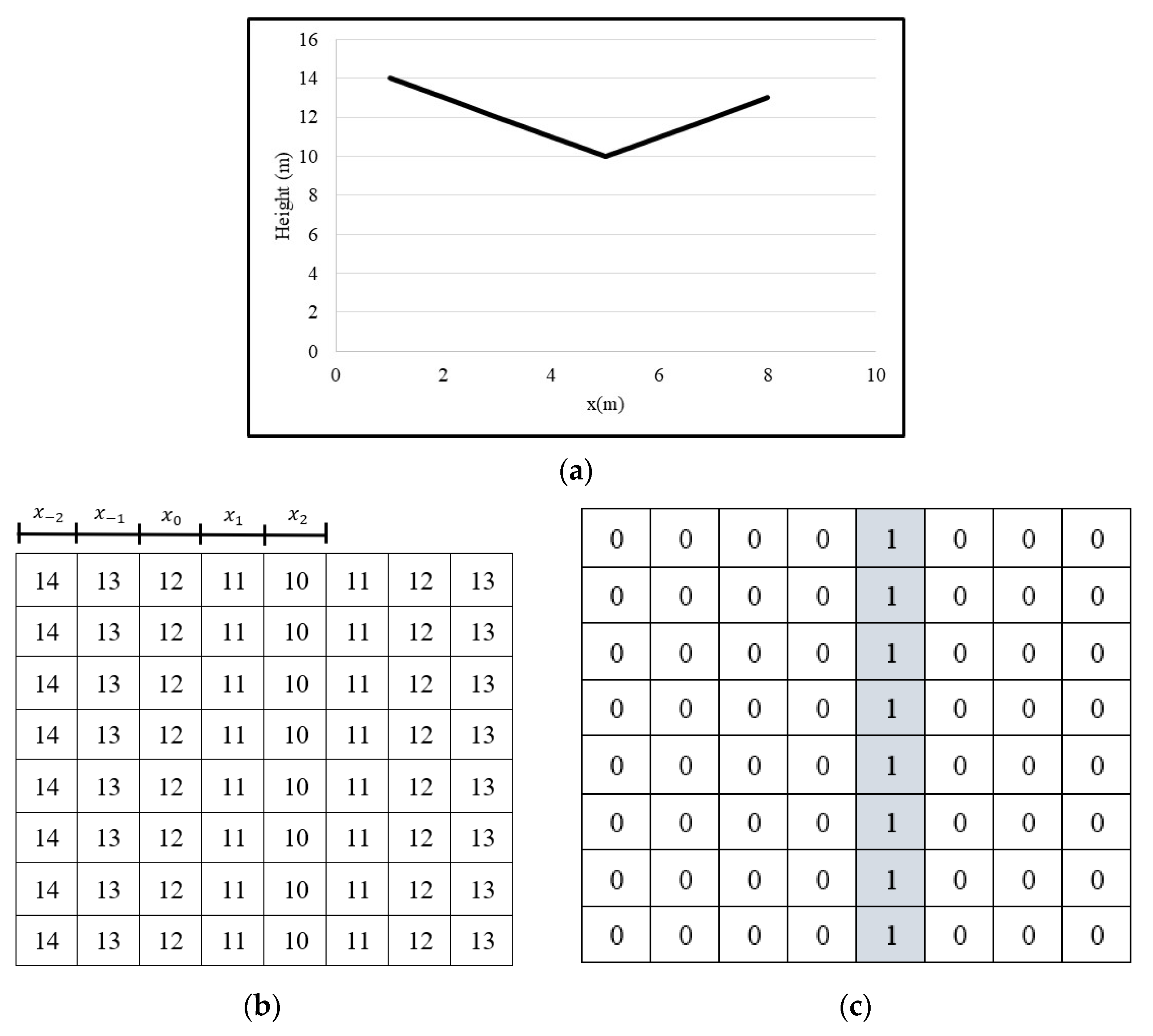
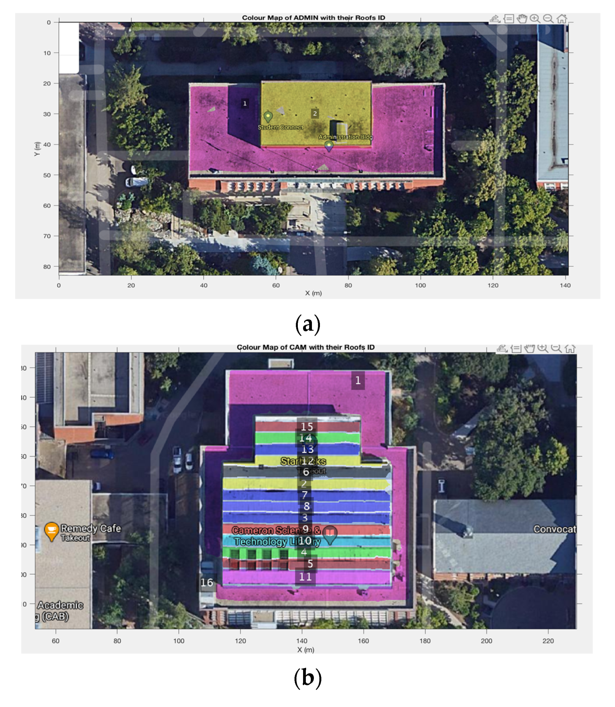
2.2.1. Roof Identification
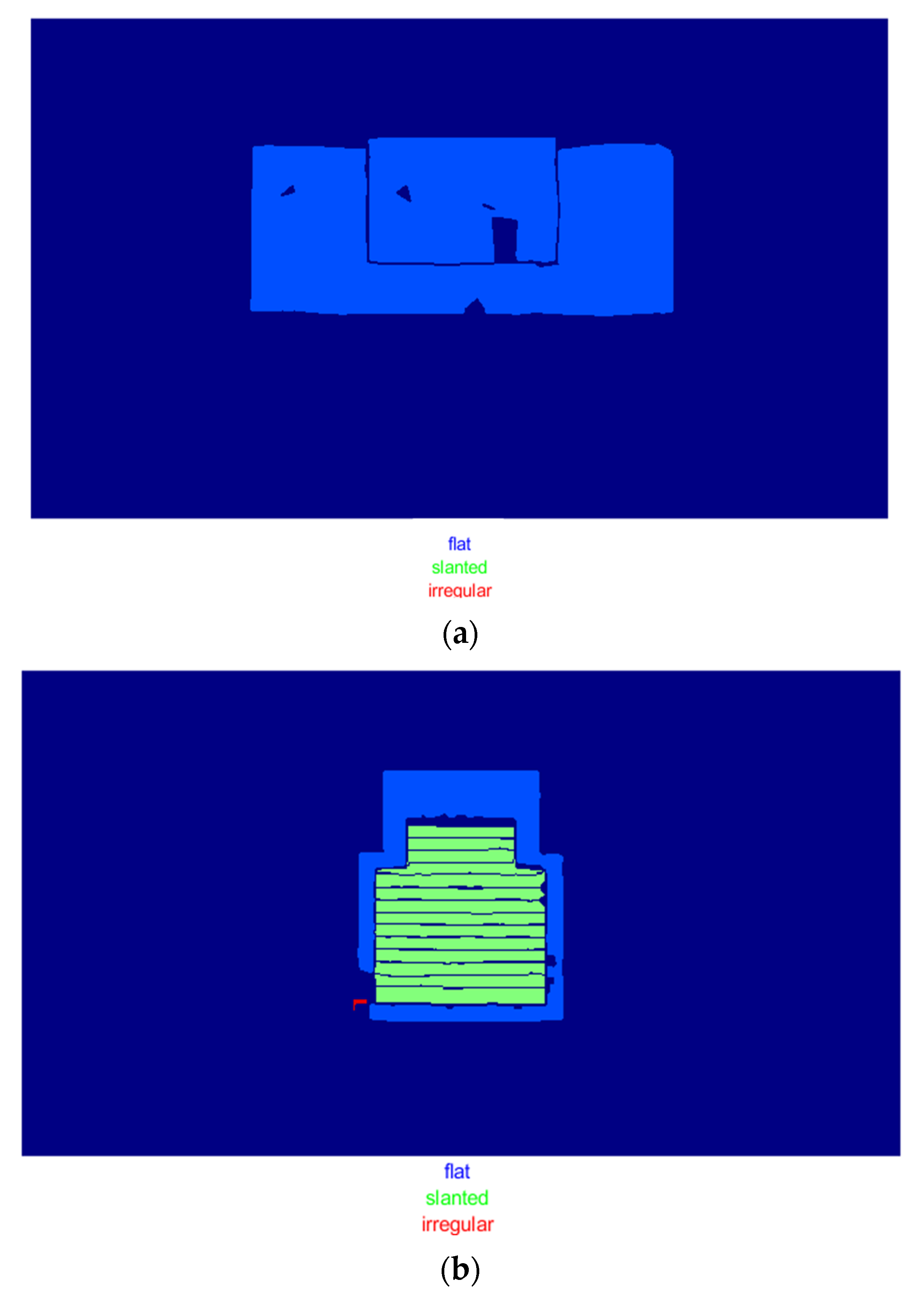
2.2.2. Roof Classification
2.2.3. Polygon Approximation
2.3. Solar Radiation Model
2.4. Multi-Objective Optimization of PV System
2.5. Data Collection
3. Results
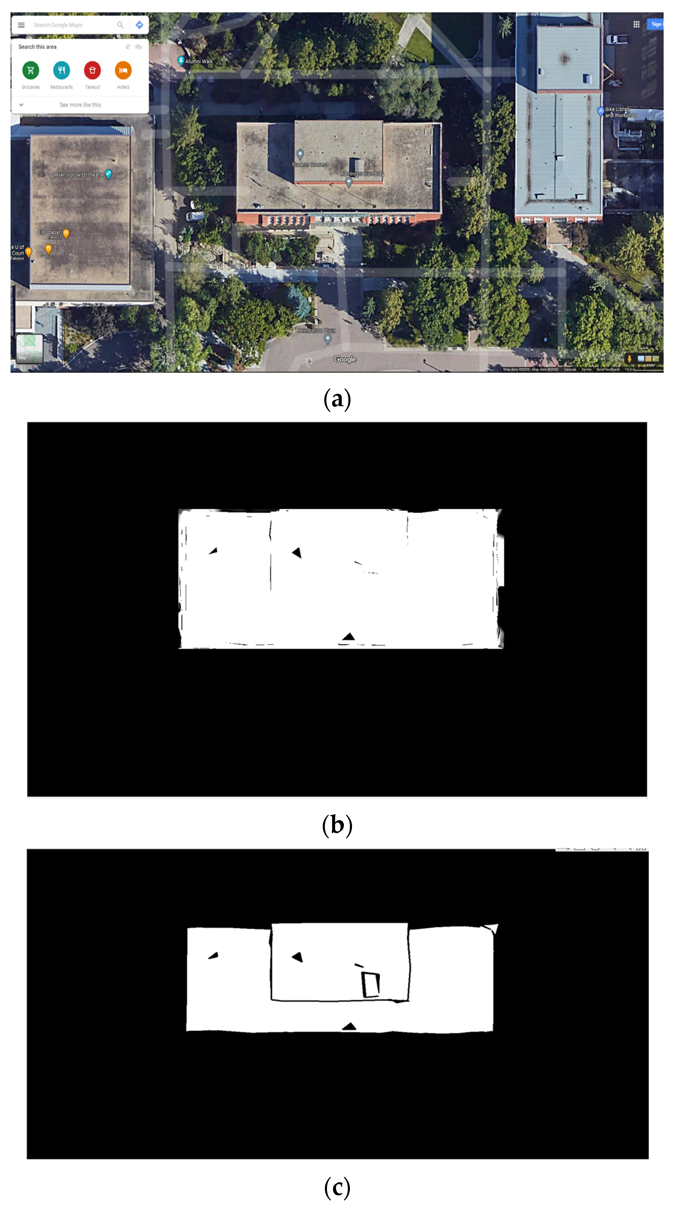
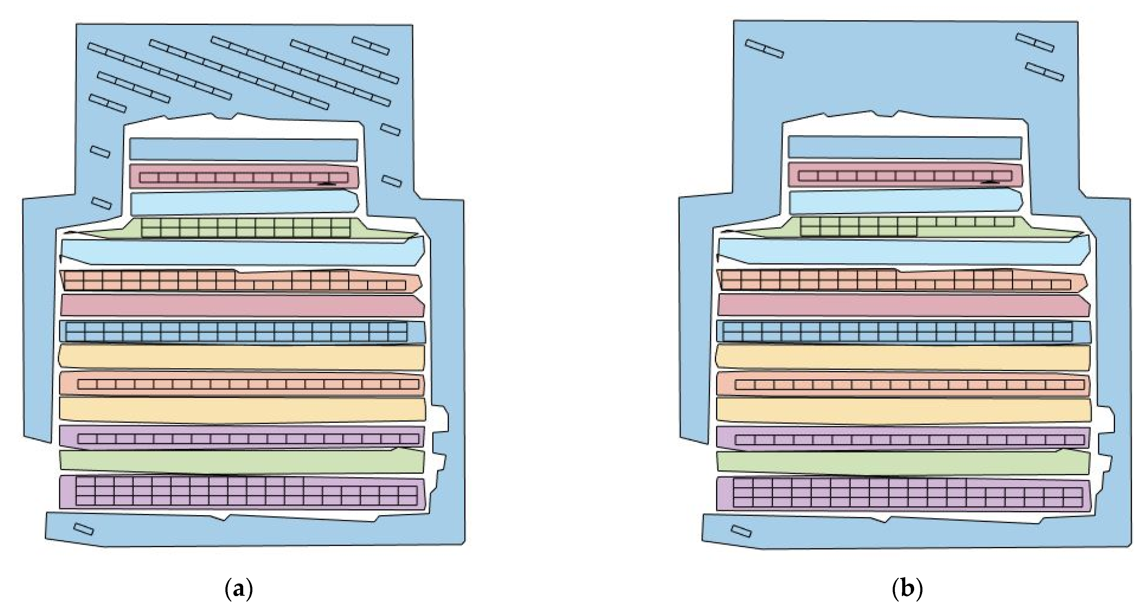
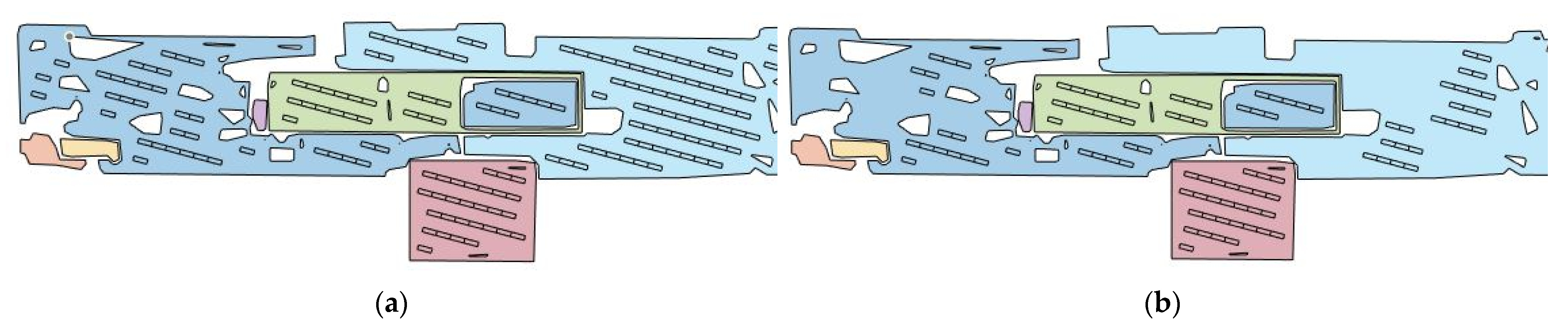
3.1. Roof Recognition
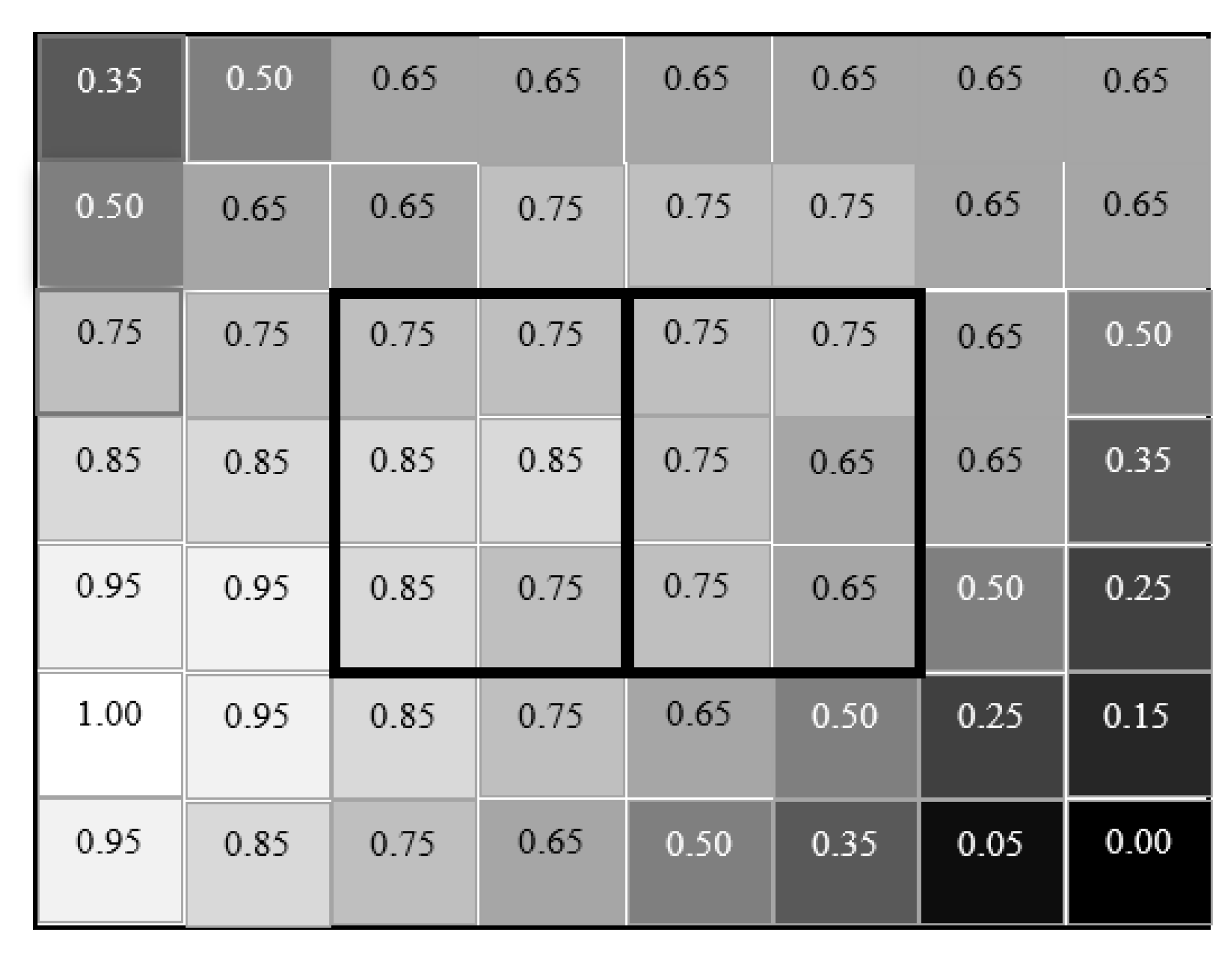
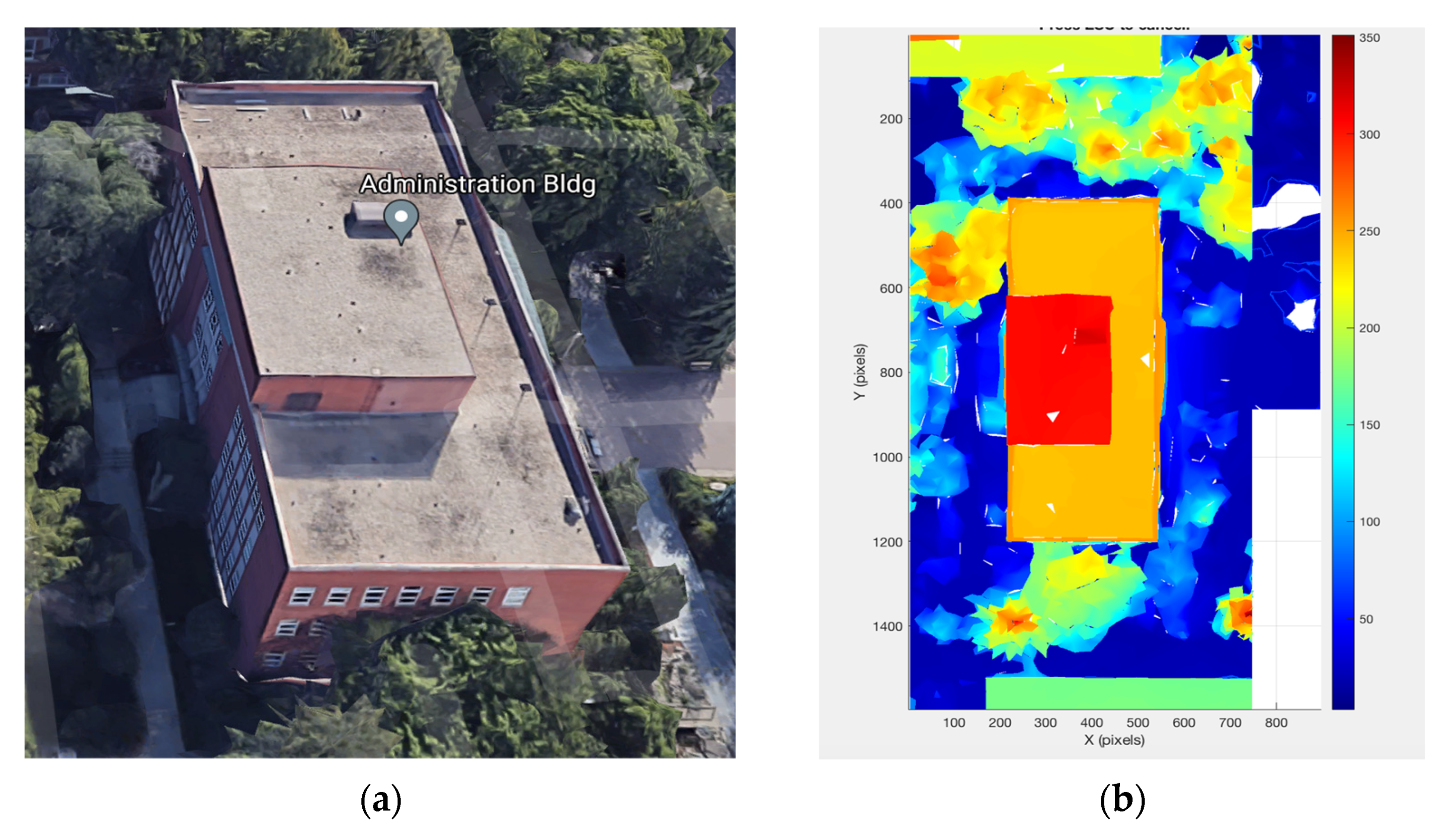
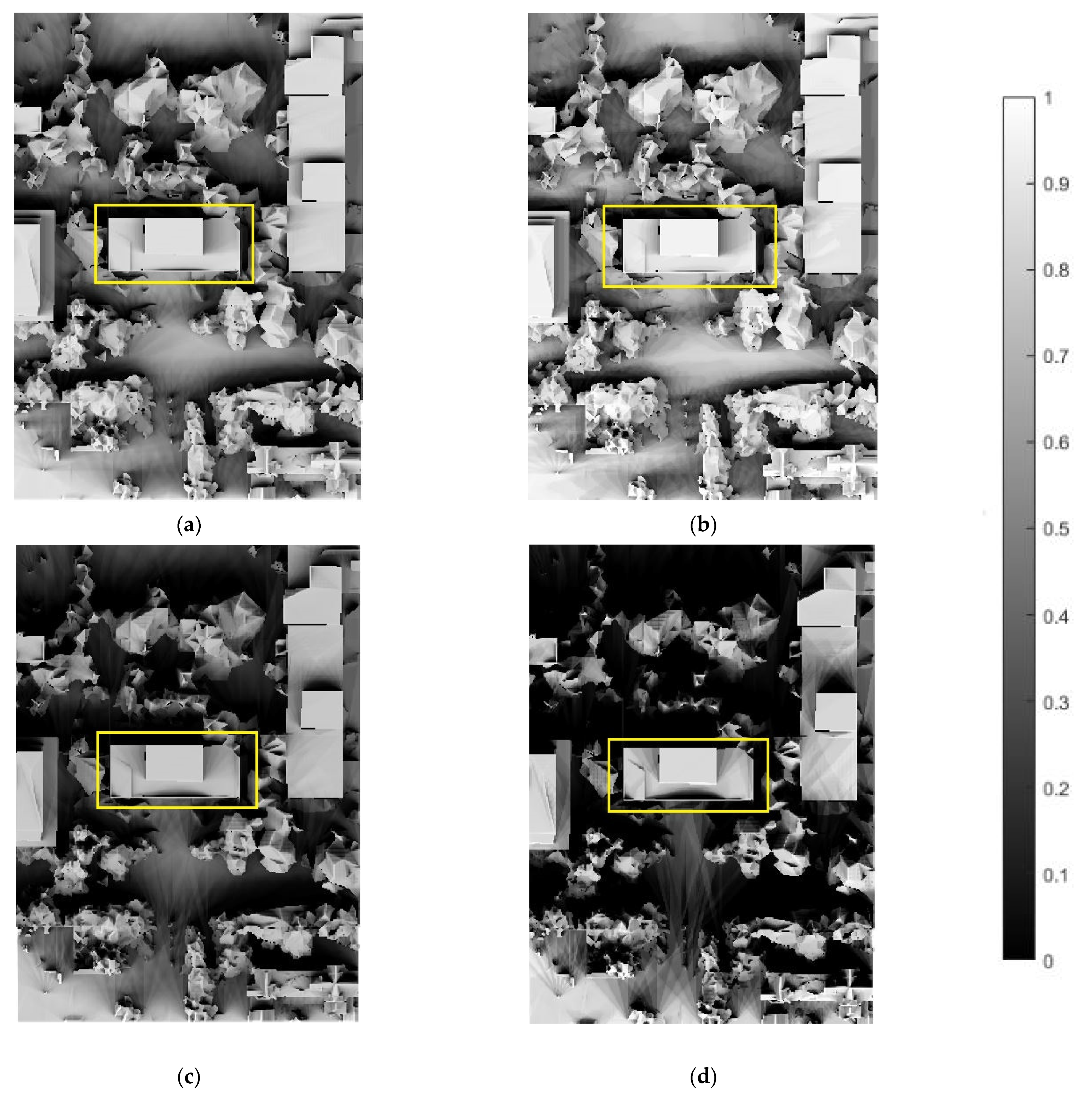
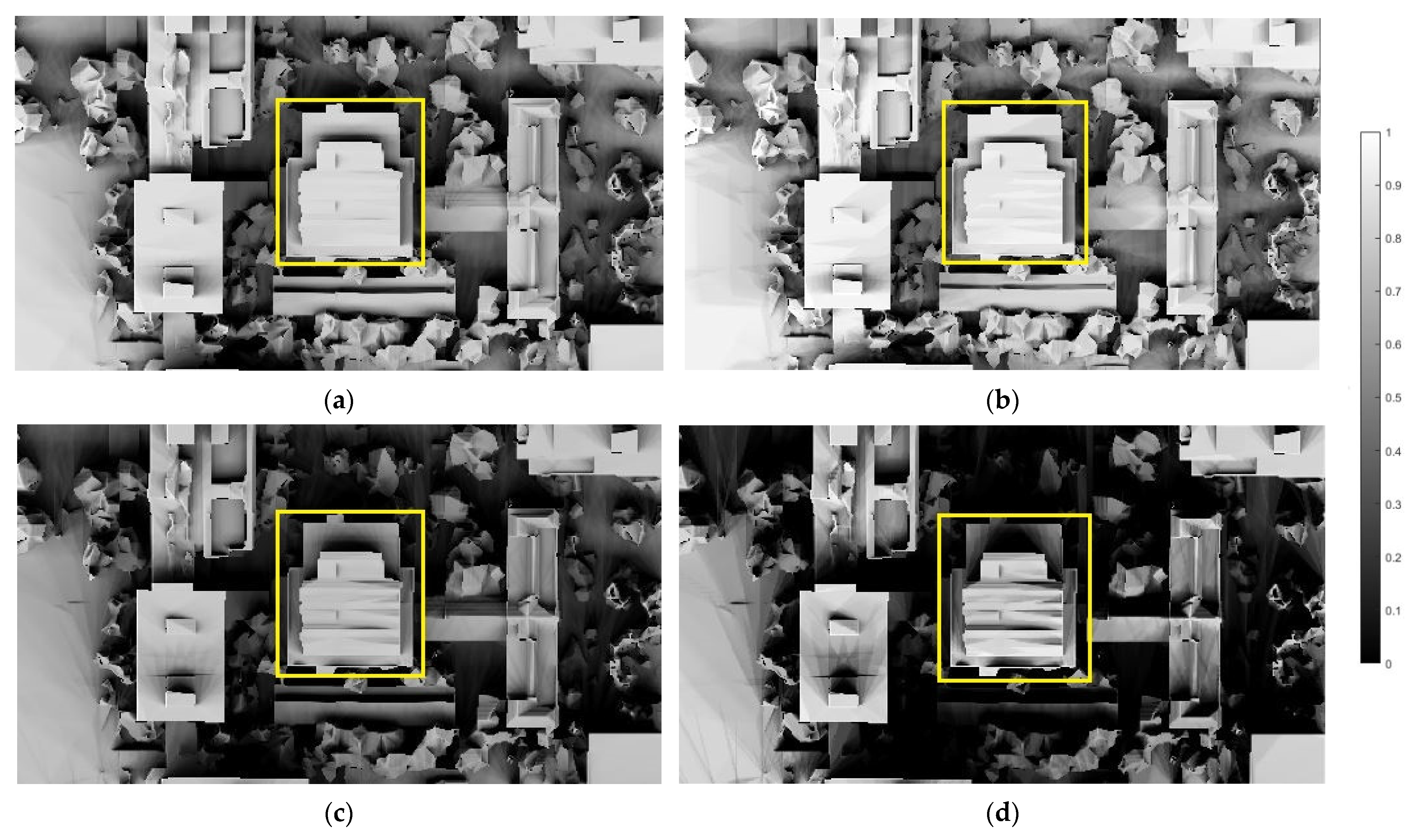
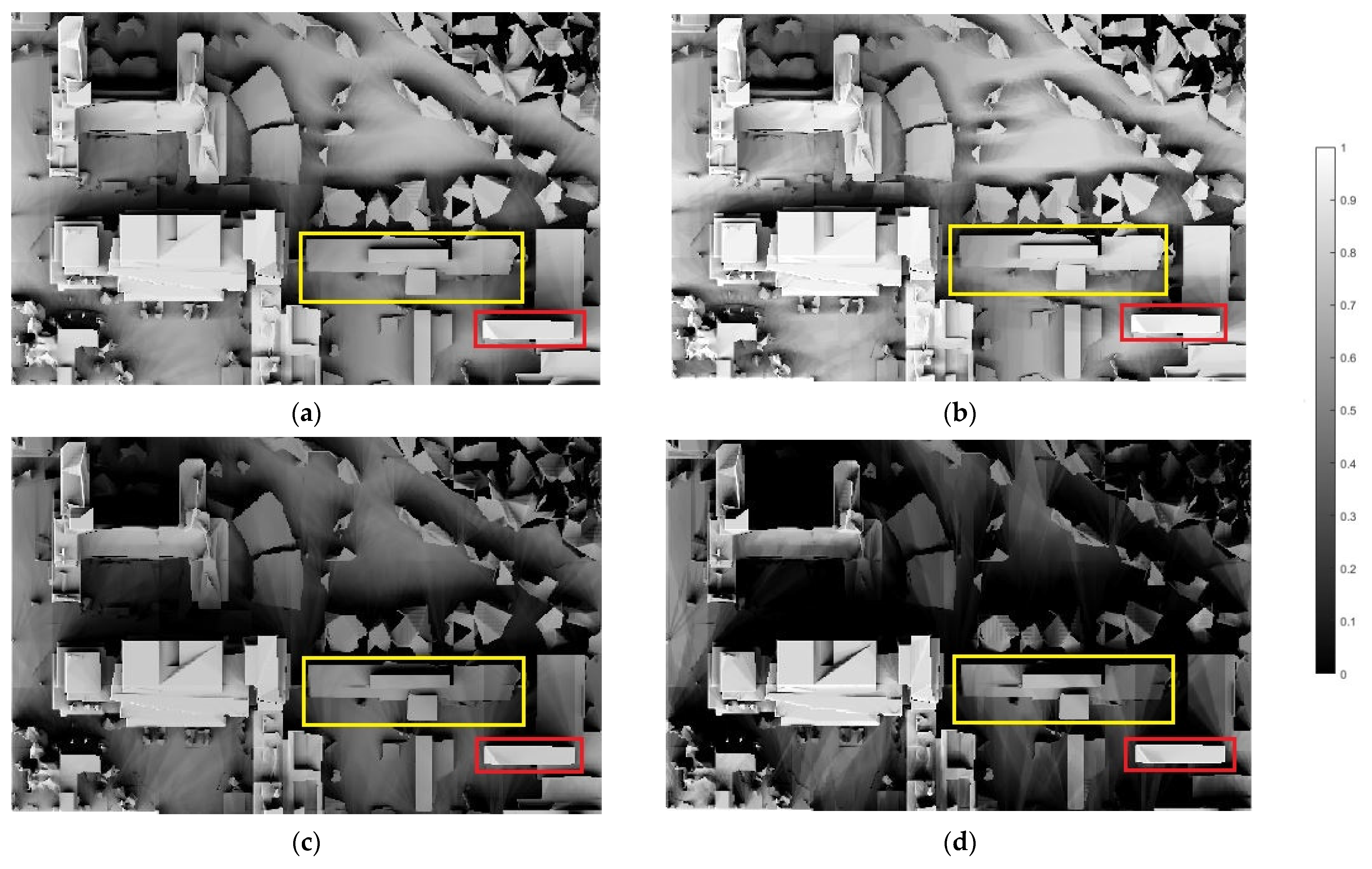
3.2. Shading Analysis Results
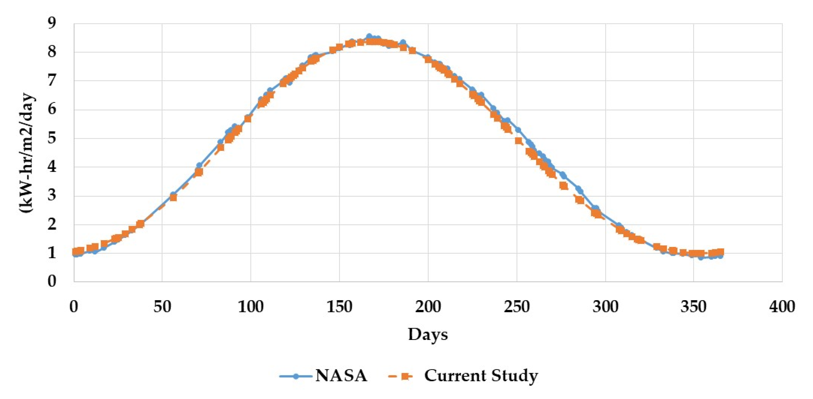
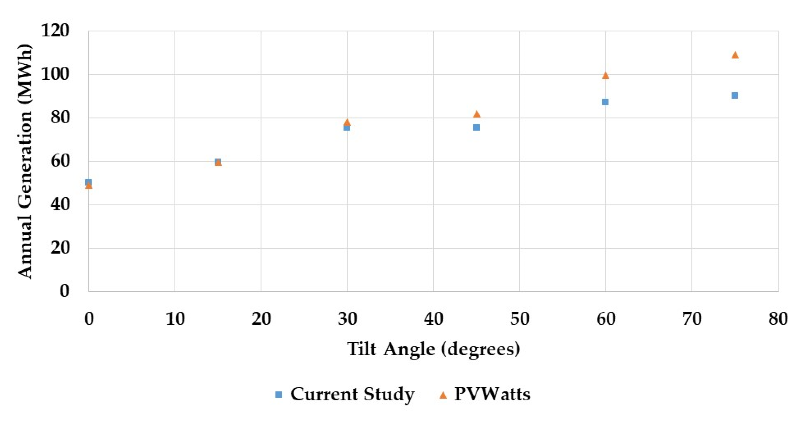
3.3. Solar Radiation Model and Annual Electricity Generation Validation
3.4. Optimization Results
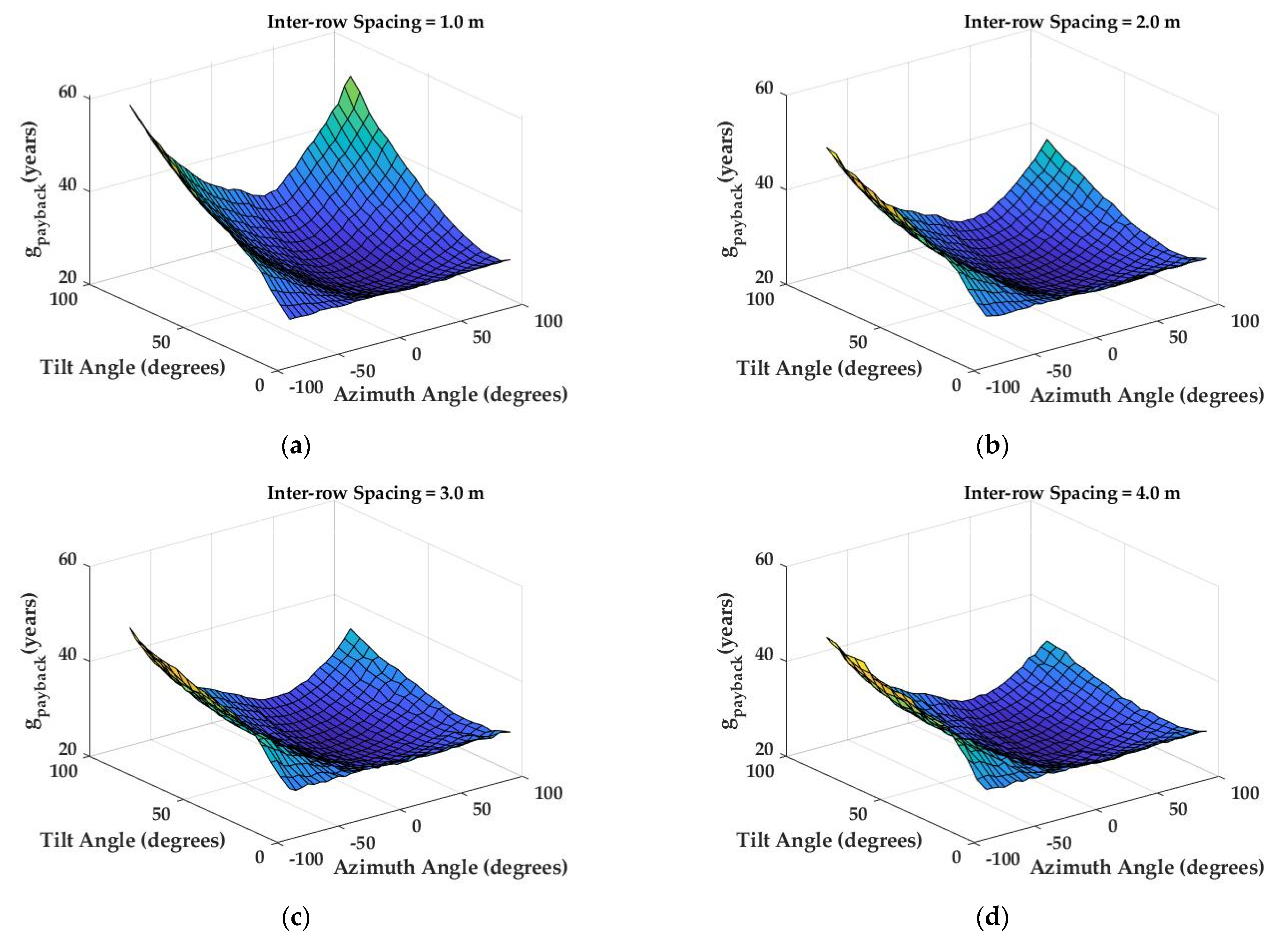
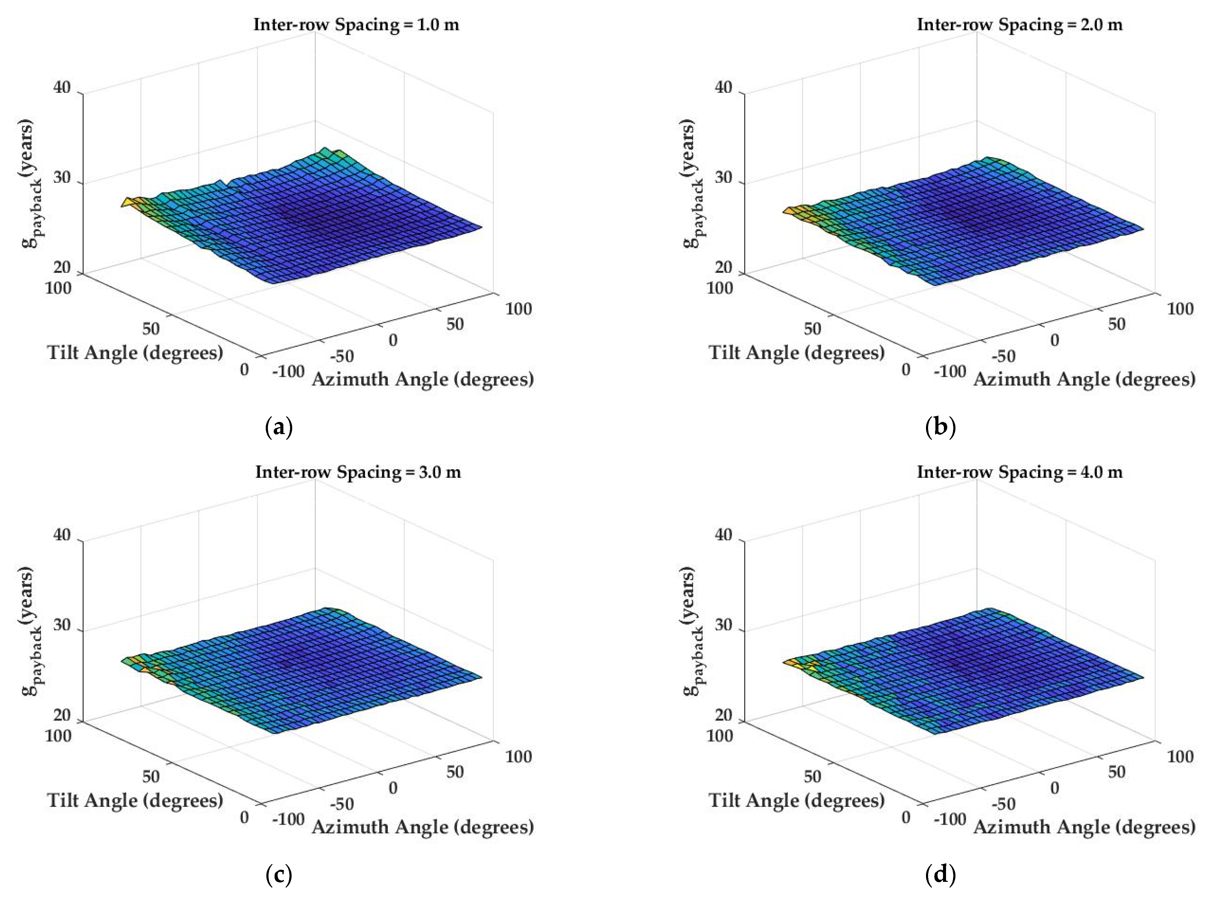
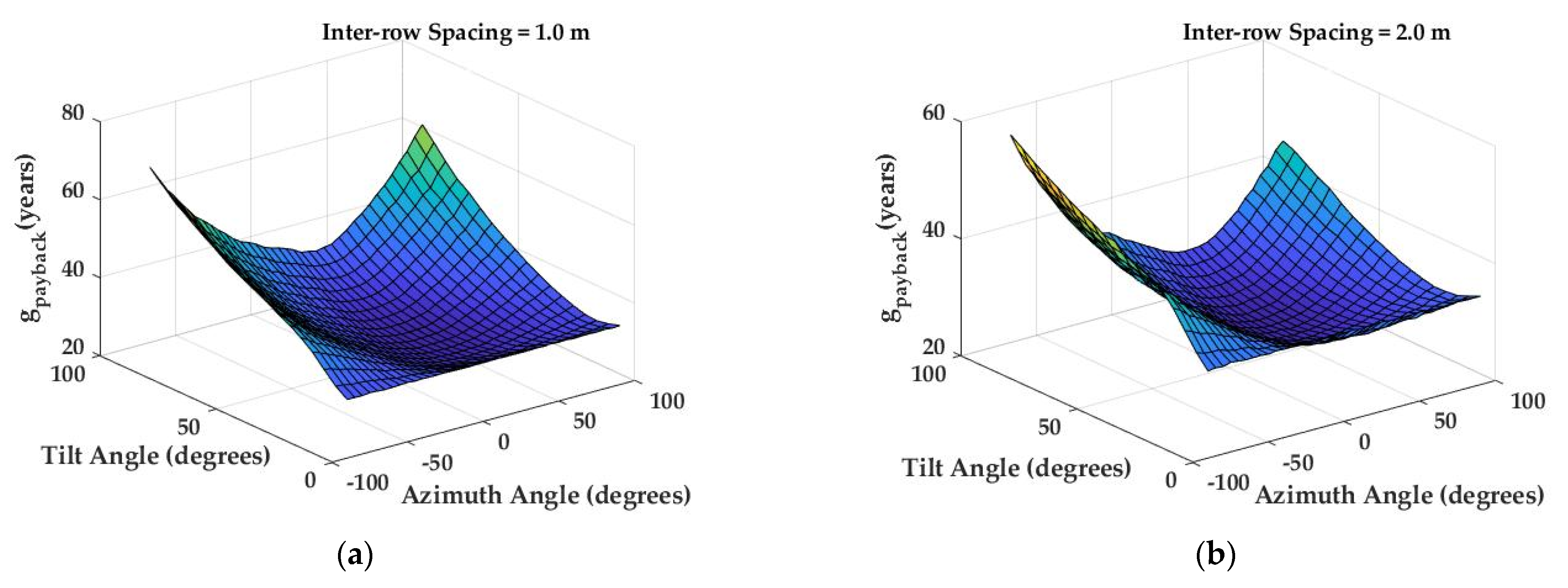
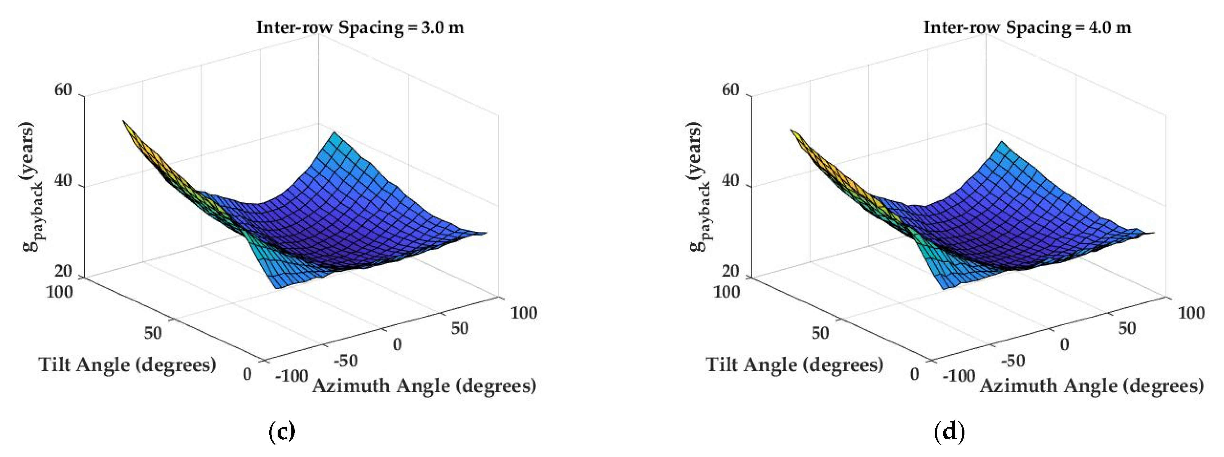
3.5. Payback Time Analysis
4. Discussion
5. Conclusions
Author Contributions
Funding
Institutional Review Board Statement
Informed Consent Statement
Data Availability Statement
Acknowledgments
Conflicts of Interest
Nomenclature
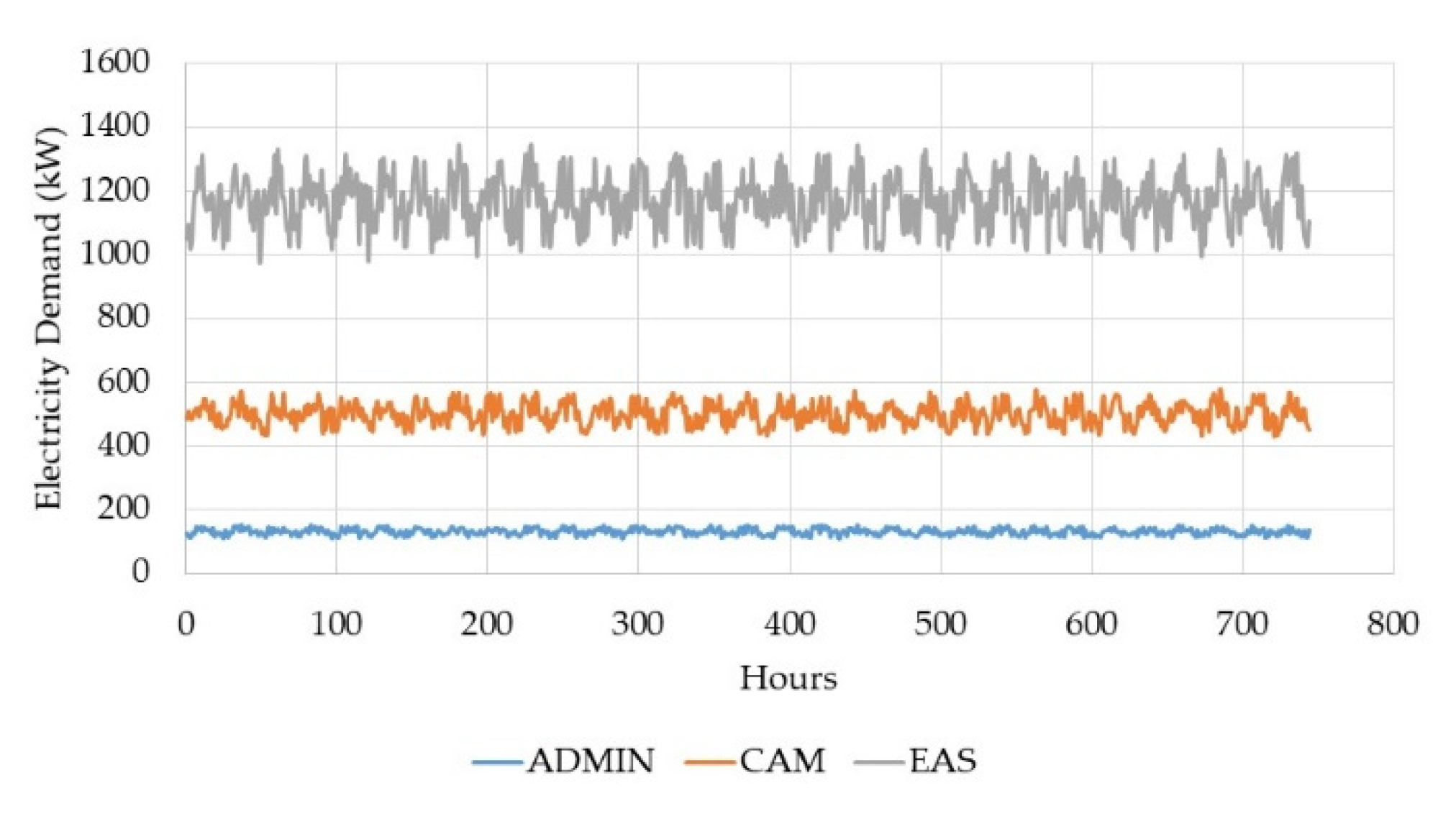
| ADMIN | Administrative building |
| Annual benefit ($) | |
| Hourly benefit ($) | |
| Pixel brightness score | |
| Yearly average of PV modules brightness scores | |
| CAM | Cameron Library building |
| Installation cost per watt ) | |
| Hourly electricity demand | |
| EAS | Earth and Atmospheric Sciences building |
| Hourly buying price of electricity from the grid | |
| Equivalent present value ($) | |
| Hourly selling price of surplus electricity | |
| Output power of the module (W/m2) | |
| Beam radiation (W/m2) | |
| Clear-sky radiation (W/m2) | |
| Diffuse radiation (W/m2) | |
| Clear-sky global horizontal radiation (W/m2) | |
| Hourly electricity generation | |
| Imported energy | |
| Extraterrestrial radiation (W/m2) | |
| PV system electricity generation | |
| Reflected radiation (W/m2) | |
| Discount or interest rate | |
| Initial cost of the photovoltaic system ($) | |
| Roof flatness | |
| Clear-sky index | |
| Inter-row spacing (m) | |
| Length of modules (m) | |
| Shadow length on the adjacent row (m) | |
| Number of years | |
| num | Number of PV panels |
| Number of shaded PV modules | |
| Number of unshaded PV modules | |
| Nominal power of modules (W) | |
| time interval | |
| Maximum overvoltage threshold | |
| Voltage at the point of common coupling | |
| Width of modules (m) | |
| Surface tilt angle ( | |
| Surface azimuth angle () | |
| Declination angle () | |
| Efficiency of the PV module | |
| Incidence angle () | |
| Zenith angle () | |
| Percentile value | |
| Surrounding reflectance | |
| Latitude of the location () | |
| Hour angle () |
Appendix A
References
- Tian, W.; Heo, Y.; De Wilde, P.; Li, Z.; Yan, D.; Park, C.S.; Feng, X.; Augenbroe, G. A review of uncertainty analysis in building energy assessment. Renew. Sustain. Energy Rev. 2018, 93, 285–301. [Google Scholar] [CrossRef] [Green Version]
- Sha, K.; Wu, S. Multilevel governance for building energy conservation in rural China. Build. Res. Inf. 2016, 44, 619–629. [Google Scholar] [CrossRef]
- Farenyuk, G. The determination of the thermal reliability criterion for building envelope structures. Teh. Glas. 2019, 13, 129–133. [Google Scholar] [CrossRef]
- Yang, H.; Lu, L. The optimum tilt angles and orientations of PV claddings for building-integrated photovoltaic (BIPV) applications. J. Sol. Energy Eng. 2007, 129, 253–255. [Google Scholar] [CrossRef] [Green Version]
- Siraki, A.G.; Pillay, P. Study of optimum tilt angles for solar panels in different latitudes for urban applications. Sol. Energy 2012, 86, 1920–1928. [Google Scholar] [CrossRef]
- Rowlands, I.H.; Kemery, B.P.; Beausoleil-Morrison, I. Optimal solar-PV tilt angle and azimuth: An Ontario (Canada) case-study. Energy Policy 2011, 39, 1397–1409. [Google Scholar] [CrossRef]
- Kaddoura, T.O.; Ramli, M.A.M.; Al-Turki, Y.A. On the estimation of the optimum tilt angle of PV panel in Saudi Arabia. Renew. Sustain. Energy Rev. 2016, 65, 626–634. [Google Scholar] [CrossRef]
- Awad, H.; Salim, K.M.E.; Gül, M. Multi-objective design of grid-tied solar photovoltaics for commercial flat rooftops using particle swarm optimization algorithm. J. Build. Eng. 2020, 28, 101080. [Google Scholar] [CrossRef]
- Zhong, Q.; Tong, D. Spatial layout optimization for solar photovoltaic (PV) panel installation. Renew. Energy 2020, 150, 1–11. [Google Scholar] [CrossRef]
- Perez-Gallardo, J.R.; Azzaro-Pantel, C.; Astier, S.; Domenech, S.; Aguilar-Lasserre, A. Ecodesign of photovoltaic grid-connected systems. Renew. Energy 2014, 64, 82–97. [Google Scholar] [CrossRef] [Green Version]
- Awad, H.; Gül, M. Load-match-driven design of solar PV systems at high latitudes in the Northern hemisphere and its impact on the grid. Sol. Energy 2018, 173, 377–397. [Google Scholar] [CrossRef]
- Alghamdi, A.S. Potential for rooftop-mounted pv power generation to meet domestic electrical demand in saudi arabia: Case Study of a villa in jeddah. Energies 2019, 12, 4411. [Google Scholar] [CrossRef] [Green Version]
- Liu, C.; Xu, W.; Li, A.; Sun, D.; Huo, H. Analysis and optimization of load matching in photovoltaic systems for zero energy buildings in different climate zones of China. J. Clean. Prod. 2019, 238, 117914. [Google Scholar] [CrossRef]
- Teofilo, A.; Radosevic, N.; Tao, Y.; Iringan, J.; Liu, C. Investigating potential rooftop solar energy generated by Leased Federal Airports in Australia: Framework and implications. J. Build. Eng. 2021, 41, 102390. [Google Scholar] [CrossRef]
- Behura, A.K.; Kumar, A.; Rajak, D.K.; Pruncu, C.I.; Lamberti, L. Towards better performances for a novel rooftop solar PV system. Sol. Energy 2021, 216, 518–529. [Google Scholar] [CrossRef]
- Litjens, G.; Worrell, E.; Van Sark, W. Influence of demand patterns on the optimal orientation of photovoltaic systems. Sol. Energy 2017, 155, 1002–1014. [Google Scholar] [CrossRef] [Green Version]
- Christiaanse, T.V.; Loonen, R.C.G.M.; Evins, R. Techno-economic optimization for grid-friendly rooftop PV systems–A case study of commercial buildings in British Columbia. Sustain. Energy Technol. Assess. 2021, 47, 101320. [Google Scholar] [CrossRef]
- Awan, A.B.; Alghassab, M.; Zubair, M.; Bhatti, A.R.; Uzair, M.; Abbas, G. Comparative Analysis of Ground-Mounted vs. Rooftop Photovoltaic Systems Optimized for Interrow Distance between Parallel Arrays. Energies 2020, 13, 3639. [Google Scholar] [CrossRef]
- Korsavi, S.S.; Zomorodian, Z.S.; Tahsildoost, M. Energy and economic performance of rooftop PV panels in the hot and dry climate of Iran. J. Clean. Prod. 2018, 174, 1204–1214. [Google Scholar] [CrossRef]
- Tiwari, A.; Meir, I.A.; Karnieli, A. Object-based image procedures for assessing the solar energy photovoltaic potential of heterogeneous rooftops using airborne LiDAR and orthophoto. Remote Sens. 2020, 12, 223. [Google Scholar] [CrossRef] [Green Version]
- Google Maps. Available online: https://www.google.com/maps/@53.526864,-113.5241896,552m/data=!3m1!1e3 (accessed on 17 November 2021).
- Nofech, J.; Narjabadifam, N.; Awad, H.; Gül, M. Mapping the solar roof potential of the North Campus buildings at the University of Alberta. In Proceedings of the 8th European Conference on Renewable Energy Systems, Istanbul, Turkey, 24–25 August 2020. [Google Scholar]
- Karlsson, B. RenderDoc Version 1.1. 2019. Available online: https://renderdoc.org/ (accessed on 29 June 2021).
- Blender Foundation. Blender: A 3D Modelling and Rendering Package; Version 2.81, Stichting; Blender Foundation: Amsterdam, The Netherlands, 2019; Available online: https://www.blender.org/ (accessed on 29 June 2021).
- Michel, E. Maps Models Importer. GitHub Repository. 2019. Available online: https://github.com/eliemichel/MapsModelsImporter (accessed on 29 June 2021).
- Soille, P. Morphological Image Analysis: Principles and Applications; Springer Science & Business Media: Berlin/Heidelberg, Germany, 2013; pp. 173–174. [Google Scholar]
- Solomon, C.; Breckon, T. Fundamentals of Digital Image Processing: A Practical Approach with Examples in Matlab; John Wiley & Sons: Hoboken, NJ, USA, 2012. [Google Scholar]
- Langford, E. Quartiles in elementary statistics. J. Stat. Educ. 2006, 14. [Google Scholar] [CrossRef]
- Van Den Boomgaard, R.; Van Balen, R. Methods for fast morphological image transforms using bitmapped binary images. CVGIP Graph. Model. Image Process. 1992, 54, 252–258. [Google Scholar] [CrossRef]
- Sreedhar, K.; Panlal, B. Enhancement of images using morphological transformation. arXiv 2012, arXiv:1203.2514. [Google Scholar] [CrossRef]
- Beyerer, J.; León, F.P.; Frese, C. Machine Vision: Automated Visual Inspection: Theory, Practice and Applications; Springer: Berlin/Heidelberg, Germany, 2015; ISBN 3662477947. [Google Scholar]
- Duffie, J.A.; Beckman, W.A. Solar Engineering of Thermal Processes, 4th ed.; John Wiley & Sons: Hoboken, NJ, USA, 2013. [Google Scholar]
- Awad, H. Integrating Solar PV Systems into Residential Buildings in Cold-climate Regions: The Impact of Energy-efficient Homes on Shaping the Future Smart Grid. Ph.D. Thesis, Univeristy of Alberta, Edmonton, AB, Canada, 2018. [Google Scholar]
- Badescu, V. Verification of some very simple clear and cloudy sky models to evaluate global solar irradiance. Sol. Energy 1997, 61, 251–264. [Google Scholar] [CrossRef]
- Kacira, M.; Simsek, M.; Babur, Y.; Demirkol, S. Determining optimum tilt angles and orientations of photovoltaic panels in Sanliurfa, Turkey. Renew. Energy 2004, 29, 1265–1275. [Google Scholar] [CrossRef]
- Bany, J.; Appelbaum, J. The effect of shading on the design of a field of solar collectors. Sol. cells 1987, 20, 201–228. [Google Scholar] [CrossRef]
- van Vuuren, D.J.; Marnewick, A.L.; Pretorius, J.H.C. A Financial Evaluation of a Multiple Inclination, Rooftop-Mounted, Photovoltaic System Where Structured Tariffs Apply: A Case Study of a South African Shopping Centre. Energies 2021, 14, 1666. [Google Scholar] [CrossRef]
- Dağtekin, M.; Kaya, D.; Öztürk, H.H.; Kiliç, F.Ç. A study of techno-economic feasibility analysis of solar photovoltaic (PV) power generation in the province of Adana in Turkey. Energy Explor. Exploit. 2014, 32, 719–735. [Google Scholar] [CrossRef] [Green Version]
- Kornelakis, A.; Marinakis, Y. Contribution for optimal sizing of grid-connected PV-systems using PSO. Renew. Energy 2010, 35, 1333–1341. [Google Scholar] [CrossRef]
- Al-Saffar, M.; Musilek, P. Reinforcement learning-based distributed BESS management for mitigating overvoltage issues in systems with high PV penetration. IEEE Trans. Smart Grid 2020, 11, 2980–2994. [Google Scholar] [CrossRef]
- Thebault, M.; Gaillard, L. Optimization of the integration of photovoltaic systems on buildings for self-consumption–Case study in France. City Environ. Interact. 2021, 10, 100057. [Google Scholar] [CrossRef]
- White, J.A.; Grasman, K.S.; Case, K.E.; Needy, K.L.; Pratt, D.B. Fundamentals of Engineering Economic Analysis; John Wiley & Sons: Hoboken, NJ, USA, 2020; ISBN 1118881060. [Google Scholar]
- Budget 2020: A Plan for Jobs and the Economy—Open Government. Available online: https://open.alberta.ca/dataset/budget-2020 (accessed on 1 October 2021).
- CanadianSolar Datasheet. Available online: https://static.csisolar.com/wp-content/uploads/2019/12/07162836/CS-Datasheet-HiKu_CS3W-P_EN.pdf (accessed on 21 June 2021).
- Constante-Flores, G.E.; Illindala, M.S. Data-driven probabilistic power flow analysis for a distribution system with renewable energy sources using Monte Carlo simulation. IEEE Trans. Ind. Appl. 2018, 55, 174–181. [Google Scholar] [CrossRef]
- POWER|Data Access Viewer. Available online: https://power.larc.nasa.gov/data-access-viewer/ (accessed on 10 August 2021).
- PVWatts Calculator. Available online: https://pvwatts.nrel.gov/pvwatts.php (accessed on 1 October 2021).
- Project Sunroof. Available online: https://sunroof.withgoogle.com/ (accessed on 28 January 2022).
- Residential and Commercial Solar Program—EnergyRates.ca. Available online: https://energyrates.ca/alberta/residential-commercial-solar-program/ (accessed on 13 November 2021).
- Residential and Commercial Solar Program in Alberta. Available online: https://alberta-solar-installers.ca/program-types/residential-and-commercial-solar-program-in-alberta (accessed on 13 November 2021).
- Prada, M.; Prada, I.F.; Cristea, M.; Popescu, D.E.; Bungău, C.; Aleya, L.; Bungău, C.C. New solutions to reduce greenhouse gas emissions through energy efficiency of buildings of special importance–Hospitals. Sci. Total Environ. 2020, 718, 137446. [Google Scholar] [CrossRef] [PubMed]
- Bungău, C.C.; Prada, I.F.; Prada, M.; Bungău, C. Design and operation of constructions: A healthy living environment-parametric studies and new solutions. Sustainability 2019, 11, 6824. [Google Scholar] [CrossRef] [Green Version]
- Bresenham, J.E. Algorithm for computer control of a digital plotter. IBM Syst. J. 1965, 4, 25–30. [Google Scholar] [CrossRef]


| Roof ID | Confidence Scores |
|---|---|
| 1 | 0.756 |
| 2 | 0.856 |
| 3 | 0.828 |
| 4 | 0.865 |
| 5 | 0.810 |
| 6 | 0.839 |
| 7 | 0.927 |
| 8 | 0.906 |
| 9 | 0.859 |
| 10 | 0.824 |
| 11 | 0.866 |
| 12 | 0.873 |
| 13 | 0.850 |
| 14 | 0.853 |
| 15 | 0.950 |
| 16 | 0.000 |
| Optimum Values of Variables | |||
|---|---|---|---|
| Variable | ADMIN * | CAM ** | EAS *** |
| (m) | 2.0 | 2.0 | 2.0 |
| (degrees) | 20 | 20 | 15 |
| (degrees) | 45 | 50 | 50 |
| Building | Annual Energy Generation (MWh) | Number of Panels | Payback (Years) |
|---|---|---|---|
| ADMIN * | 35.13 | 73 | 22.99 |
| CAM ** | 75.28 | 185 | 27.20 |
| EAS *** | 41.95 | 102 | 26.91 |
| Building | Panels Number with Obstacles Shading | Panels Number without Obstacles Shading | PV System Annual Output (MWh) with Obstacles Shading | PV System Annual Output (MWh) without Obstacles Shading | Percentage of Generation Difference (%) |
|---|---|---|---|---|---|
| ADMIN * | 73 | 80 | 35.13 | 48.88 | 28.13 |
| CAM ** | 185 | 230 | 75.28 | 123.06 | 38.83 |
| EAS *** | 102 | 178 | 41.95 | 107.97 | 61.14 |
| Building | Payback without Incentives (Years) | Payback with Incentives (Years) |
|---|---|---|
| ADMIN * | 22.99 | 16.82 |
| CAM ** | 27.20 | 19.90 |
| EAS *** | 26.91 | 19.69 |
Publisher’s Note: MDPI stays neutral with regard to jurisdictional claims in published maps and institutional affiliations. |
© 2022 by the authors. Licensee MDPI, Basel, Switzerland. This article is an open access article distributed under the terms and conditions of the Creative Commons Attribution (CC BY) license (https://creativecommons.org/licenses/by/4.0/).
Share and Cite
Narjabadifam, N.; Al-Saffar, M.; Zhang, Y.; Nofech, J.; Cen, A.C.; Awad, H.; Versteege, M.; Gül, M. Framework for Mapping and Optimizing the Solar Rooftop Potential of Buildings in Urban Systems. Energies 2022, 15, 1738. https://doi.org/10.3390/en15051738
Narjabadifam N, Al-Saffar M, Zhang Y, Nofech J, Cen AC, Awad H, Versteege M, Gül M. Framework for Mapping and Optimizing the Solar Rooftop Potential of Buildings in Urban Systems. Energies. 2022; 15(5):1738. https://doi.org/10.3390/en15051738
Chicago/Turabian StyleNarjabadifam, Nima, Mohammed Al-Saffar, Yongquan Zhang, Joseph Nofech, Asdrubal Cheng Cen, Hadia Awad, Michael Versteege, and Mustafa Gül. 2022. "Framework for Mapping and Optimizing the Solar Rooftop Potential of Buildings in Urban Systems" Energies 15, no. 5: 1738. https://doi.org/10.3390/en15051738
APA StyleNarjabadifam, N., Al-Saffar, M., Zhang, Y., Nofech, J., Cen, A. C., Awad, H., Versteege, M., & Gül, M. (2022). Framework for Mapping and Optimizing the Solar Rooftop Potential of Buildings in Urban Systems. Energies, 15(5), 1738. https://doi.org/10.3390/en15051738