Abstract
Architectural space layout has proven to be influential on building energy performance. However, the relationship between different space layouts and their consequent energy demands has not yet been systematically studied. This study thoroughly investigates such a relationship. In order to do so, a computational method was developed, which includes a method to generate space layouts featuring energy-related variables and an assessment method for energy demand. Additionally, a design of experiments was performed, and its results were used to analyse the relationship between space layouts and energy demands. In order to identify their relationship, four types of design indicators of space layout were proposed, both for the overall layout and for each function. Finally, several optimisations were performed to minimise heating, cooling and lighting demands. The optimisation results showed that the maximum reduction between different layouts was up to 54% for lighting demand, 51% for heating demand and 38% for cooling demand. The relationship analysis shows that when comparing the four types of design indicators, the façade area-to-floor area ratio showed a stronger correlation with energy demands than the façade area ratio, floor area ratio and height-to-depth ratio. Overall, this study shows that designing a space layout helps to reduce energy demands for heating, cooling and lighting, and also provides a reference for other researchers and designers to optimise space layout with improved energy performance.
1. Introduction
Space layout design is one of the most important tasks in architectural design, taking place around ‘scheme design’ and ‘design development’ in the early design phase [1]. It refers to the allocation of different functions within the building plan, and it is based on the placement of interior partitions as well as exterior walls. Some studies showed that space layout impacts building energy performance greatly. In [2], five space layouts for an office building in the UK were compared, and a difference of up to 57% in the heating demand for peak winter and up to 67% in the lighting demand for peak summer were found. In [3], various layouts for a library building in Turkey with the same geometry were simulated and compared; the results showed a difference of up to 19% for the heating demand of one day, up to 20% for the cooling demand of one day and up to 10% for the lighting demand of one day. Additionally, the building sector—especially commercial building—has been proven to have significant potential in reducing carbon emissions [4]. The study of [5] also shows that the energy demands of commercial buildings will increase at a relatively faster speed than residential buildings. As one important design task of building design, it is meaningful to fully identify the potential of space layout to reduce carbon emissions and energy consumption in office buildings.
With the recent advances in computational fields, performative computational architecture (PCA) has become ever more popular for architectural design and has shown high potential in improving building performance [6]. With PCA, the building’s geometric and material properties are parametrised, and designers vary the design variables to satisfy the design objectives relevant to certain building performance. Different design variables of buildings have been explored for PCA, including geometry, façade properties, materials, shading, orientation, window to wall ratio (WWR), etc. Recent studies have proven that using PCA to optimise building energy performance helps to reduce energy demands highly, as shown in [7].
Some studies showed the potential of designing space layout with PCA to improve the energy performance of buildings. The study of [3] optimised space layouts with the objective of improving energy and daylighting performance, as well as the functionality of the layout. The study of [8] developed a method for automatically generating the space layout with improved thermal performance. However, among the studies relevant to space layout design, only a few focused on energy performance, as shown in the review study of [9]. Similarly, among the studies for building energy performance optimisation, only a few focused on space layout design, as shown in the review study of [6]. Furthermore, among the few studies that considered both space layout design and energy performance as analysed in the review study of [9], none evaluated the relationship between space layout and energy demand.
Therefore, space layout has proven to have an impact on building energy performance. However, the relationship between different space layouts and the consequent energy demands has not been systematically studied, and few studies have applied PCA to space layout design. In order to solve this research gap, this paper presents a study for identifying the relationship between space layout and energy performance and for illustrating how to optimise space layout design with improved energy performance, as well as investigating how much energy demand can be reduced from the optimisation.
As for the scope of this study, although space layout affects several aspects of building performance, such as safety, logistics, adjacency, connection, view and acoustics [10], this study intentionally focuses solely on energy. This is because building knowledge of the relationship between space layout and energy performance is the first required step, and can be used later for the broader integration of energy with other performances.
In order to investigate the relationship between space layout and energy performance, the design of experiments (DOE) method was used in this study. DOE is an experiment that refers to a series of tests in which the input variable values are changed according to a certain rule, in order to identify the reasons for the changes in outputs [11]. Additionally, optimisations were also run in this study to find the space layout with the best energy performance. Based on the results of DOE and optimisations, the relationship between space layout and energy performance can be identified.
The structure of this paper is as follows: The computational method for DOE and optimisation of space layout design used in this study is described in Section 2. Section 3 proposes the design indicators representing the characteristics of space layouts. The generated layouts using the DOE method are used to analyse the relationship between space layout and energy demand in Section 4. Finally, the optimisations for minimising heating, cooling and lighting demands are shown in Section 5.
2. Method for DOE and Optimisation
The computational method for DOE and optimisation includes three parts: the generation of space layout featuring energy-related variables, the energy and daylight performance assessment, and the computational analysis of results. The automation of the computational method was achieved by using a commercially available software workflow. The workflow of the method and three parts are explained in the following sub-sections. Once the overall method was set, it allowed the authors to run DOE and analyse the relationship between space layout and energy demand based on DOE results, as well as the optimisation for minimising energy demands.
2.1. Computational Workflow of the Method
The method was implemented with a computational workflow that integrated Grasshopper (GH) [12] with modeFRONTIER (mF) [13], as shown in [14]. The energy and daylighting simulation was performed in GH using Ladybug Tools, specifically Honeybee [15], which uses Radiance (5.2.1) [16] and Daysim [17] for daylight simulation and EnergyPlus (9.0.0) [18] for energy simulation. EnergyPlus has been proven to have a low accuracy in daylight simulation [19], so its integration with Radiance and Daysim is necessary for this study. MF was used to process the automation of the entire workflow, optimisation, data postprocess and analysis. As shown in Figure 1, the computational workflow is presented as follows:
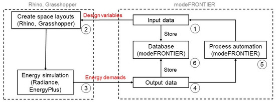
Figure 1.
Workflow of the computational method for DOE and optimisation.
- (1)
- A set of design variables (used to control the form of space layout as described in Section 2.4.1) was input to GH;
- (2)
- Based on the inputs, the space layout was generated in GH;
- (3)
- The as-generated space layout was simulated for annual heating, cooling and lighting demands in Radiance/Daysim and EnergyPlus, with the climate data of Amsterdam;
- (4)
- The calculated energy demands were sent to mF and used as outputs of DOE or further defined as design objectives for optimisation;
- (5)
- The process continued in mF, based on optimisation algorithms or a set of evaluations designed for DOE, then new design variables were sent back to GH and the loop continued;
- (6)
- With the iteration of the integration process, the input data and output data were saved in the database, which later was used for relationship analysis.
Additionally, the detailed workflow and screenshots of used tools are shown in Figure 2, which will be explained in the following subsections.
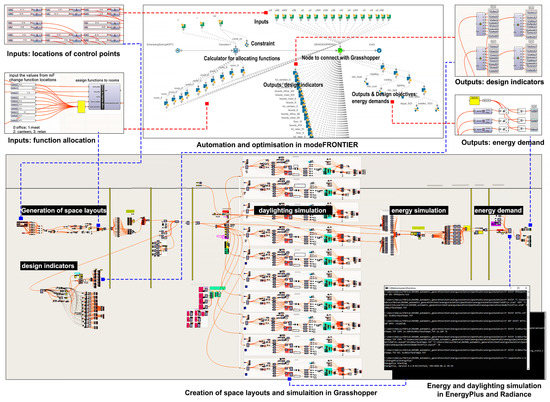
Figure 2.
Workflow of the computational method and screenshots of used tools.
2.2. Generation of Space Layout
As explained in the Introduction, although space layout can impact some functional performance, such as adjacency, connection and logistic, this study focuses solely on design variables of space layout which are directly relevant for energy, and does not include other variables. Therefore, some layouts with rather extreme geometric properties are allowed in this section and this study.
The design variables of space layout can be classified into those with a fixed layout boundary and those with a non-fixed layout boundary, as shown in [9]. In order to include and test large sets of design variables, design variables with a non-fixed layout boundary were used for the generation of the space layout in this study. Therefore, the layout boundary, interior partition and function allocation were varied, which helped to change the properties of both rooms and the layout. Changing the layout boundary also resulted in the change of the room orientation and depth. In order to better compare different rooms for their design indicators and energy demands, it was necessary to keep the room area the same. Therefore, the layout was split into 10 rooms with the same room area.
The method for generating the layout was developed based on a reference layout, which was previously published by the authors [20]. The layout included 12 rooms, i.e., 6 offices, 2 meeting rooms, 1 canteen, 1 break room, 1 core and 1 staircase. Each room was 9 m wide and 9 m deep. The core and staircase were located in the middle, and in this way, most rooms could be connected by the core and staircase. The corridor was not considered in this layout.
The detailed steps for generating the space layout are shown in Figure 3. The starting layout is shown in Figure 3a, and its floor area is 972 m2 which was kept fixed during the following steps. The procedure for changing layouts is shown as follows.
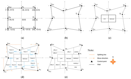
Figure 3.
Procedure for generating layouts. (a) Original layout; (b) Changing the layout boundary using control points; (c) Locating the core and staircase in the middle; (d) Splitting the remaining layout into 10 rooms with the same area; (e) Allocating functions to the 10 rooms.
2.2.1. Changing Layout Boundary
Eight points were used to control the layout boundary, in order to change floor area and façade area in different orientations, as shown in Figure 3b. Each point could move along the x axis for a maximum of 8.5 m left and 8.5 m right, and along the y axis for a maximum of 6.5 m up and 6.5 m down, with an intermediate step of 1.0 m. The points controlled the variation of the layout boundary in eight orientations, i.e., S, SE, E, NE, N, NW, W and SW.
2.2.2. Locating Core and Staircase
After the layout boundary was changed, the layout was then split into rooms. As shown in Figure 3c, two square rooms were located in the middle of the layout and used as core and staircase, with the original point as the middle point of their adjacent boundary. The room area of core and staircase was kept at 1/12 of the total layout area.
2.2.3. Splitting the Remaining Layout
As shown in Figure 3d, the remaining layout was split into 10 rooms as follows: Line-0 (the horizontal line starting from the vertex of the staircase) was used as the starting line, and the splitting line moved in a counter-clockwise direction until the area covered by Line-0, the splitting line and layout boundary was larger than 1/12 of the layout area and the current splitting line was Line-1 and the split room was Room-0; the splitting line continued moving until the area covered by Line-1, the splitting line and layout boundary was larger than 1/12 of the layout area and the current splitting line was Line-2 and the split room was Room-1; the splitting line continued moving until all 10 rooms were created. When the splitting line arrived around one corner of the layout, if the covered area was not big enough for one room with the splitting line moving, the splitting line rotated 90° in counterclockwise direction to continue splitting until the split-room area was large enough. In order to ensure that the splitting algorithm worked well, a test was added: if the room-area difference between two rooms was greater than 10%, then the layout generated was reported as an error, the following steps were skipped and this layout was omitted to save computational time.
Although the algorithm considered different scenarios with different layout shapes, one scenario was disregarded, as shown in Figure 4: when using Line 5 to split the SW corner, a concave shape appeared and both rooms, i.e., S0 (20 m2) and S1 (49 m2), were not big enough as a single room (58 m2), while the sum of the two rooms (69 m2) was bigger than a room; this situation was ignored in this study.
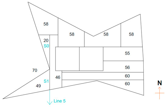
Figure 4.
Ignored scenario for splitting the layout. Note: The numbers (m2) in the layout are the corresponding room areas.
2.2.4. Allocating Functions
After the remaining layout was split into 10 rooms, the 4 functions, i.e., office, meeting room, canteen and break room, were then allocated to the 10 rooms, as shown in Figure 3e. This step was accomplished with a calculator in mF, as shown in Figure 2. The allocating procedure was as follows: first, 1 room from the 10 rooms was selected as canteen; then another room from the remaining 9 rooms was selected as break room; after this, 2 more rooms from the remaining 8 rooms were selected as meeting rooms; finally, the remaining 6 rooms were used as offices. After this step, the layout was generated and was input to Radiance/Daysim and EnergyPlus for daylight and energy simulation.
2.3. Energy and Daylight Performance Assessment
The third step of the computational method regards the performance assessment based on simulation. In this study, the annual heating, cooling and lighting demands for the whole layout were used to assess the energy performance. The detailed information about energy and daylight performance simulation were shown in our previous study [20]. The temperate climate data of Amsterdam in the Netherlands was used.
Daylight simulation and energy simulation were integrated in this study. The electric lighting schedule was calculated based on the difference between the target illuminance and the received daylight illuminance, and energy simulation was performed based on the calculated lighting schedule. Additionally, shading was considered for daylight simulation. The screen installed outside the windows was used for shading on all facades, and external vertical illuminance was used to determine the state of shading system.
An outdoor air flow rate of 0.37 dm3/s·m2 and an extra 8.89 dm3/s·person were used for ventilation [21], with a humidity threshold of 25–60% [22]. To save the energy consumption for ventilation, a heat exchanger with an efficiency of 0.7 was added. An infiltration rate of 0.2 ACH was assigned for most rooms, except for the middle rooms. The occupancy and equipment load density were important to determine thermal demands. For office, meeting room, canteen, break room, staircase and core, their maximum occupancies (persons/room) were 6, 12, 9, 9, 3 and 3, respectively, and their maximum equipment load densities (W/m2) were 6.9, 4, 48, 0.8, 0 and 3, respectively. These values were collected based on the reference of [23].
More detailed information about the simulation is shown in Table 1 regarding constructions, glazing properties and reflectance of interior surfaces. The constructions were assigned according to the local building design standards in the Netherlands. In addition, the set points of different functions for heating, cooling and lighting, as well as the occupancy schedule are also presented in Table 1. The heat flow between different floors was not considered, thus floors and ceilings were adiabatic. The WWR of the simulation model was kept at 40%.

Table 1.
Detailed information for simulation, adapted from [20].
Different from our previous work [20] which took into account a geometrically fixed layout, the daylight simulation model of the study dynamically separated one room into three lighting zones based on yearly daylight illuminance. Similarly, as for the room with different façade orientations, its windows were assigned to two different shading groups, the maximum number allowed by Ladybug tools. In the case of rooms which had more than two façade orientations, such as some corner rooms, their windows with the smallest angle difference between their façade normal were grouped together.
In order to save computational time for the huge amount of simulation used in DOE and optimisation, this study used less-accurate daylight simulation parameters. The test-points were located at a distance of 1.5 m. Radiance parameters were as follows: ab (ambient bounces) was 2, ad (ambient divisions) was 512, as (ambient super-samples) was 128, ar (ambient resolution) was 16, and aa (ambient accuracy) was 0.25 [24]. As full interior solar distribution cannot be handled correctly for a concave shape in EnergyPlus, the ‘full exterior with reflections’ was used for solar distribution, as explained in [16].
2.4. Iterative Generation and Assessment
The final step of the computational method entailed an automated iterative loop of space layout generation and energy performance assessment. The process looped generation and assessment, based on an optimisation algorithm or a set of evaluations designed for DOE. As shown in Figure 1 and Figure 2, the input data (i.e., design variables) and output data were used to process automation.
2.4.1. Design Variables
As shown in Table 2, the design variables included two categories, i.e., those for changing layout boundary, as explained in Section 2.2.1; and those for changing function allocation, as explained in Section 2.2.4. The design variables for the layout boundary were the values that the eight control points changed along the x and y axis with an interval of 1 m. Regarding the variables for function allocation, two design variables (c and r) represent the locations of canteen and break room, respectively, and one vector input variable (mr) included two design variables (mr[0] and mr[1]), which represented the locations of two meeting rooms, respectively.
Table 2.
Design variables and their domains.
2.4.2. Outputs and Constraints
The outputs included annual heating demand, cooling demand and lighting demand of the whole layout per floor area. In mF, the outputs were manually chosen to be ‘min’ in the interface, i.e., minimising energy demands were the design objectives for optimisation. Two constraints were also added in mF: one for layout area, i.e., changing the layout variant within a 5% difference of the floor area of the reference layout (923 m2 to 1021 m2); and one to avoid two meeting rooms located in the same room. A detailed description of outputs and constraints is shown in Table 3.
Table 3.
Outputs and constraints.
2.5. Concurrent Evaluations
As shown in the study [9], computational time is a big issue for energy performance optimisation. The computational time for each evaluation in this study was quite high, varying from 1 h to 2 h depending on the computer property used. In order to speed up simulation and reduce the total computational time, four computers were used simultaneously, i.e., four concurrent evaluations were run at the same time. The details of the four computers are as follows: one computer used 2 Intel(R) Xeon(R) CPUs (E5-2680 v2 @ 2.80 GHz), with 20 cores and 40 logical processors; two computers used 2 Intel(R) Xeon(R) CPUs (E5-2680 v3 @ 2.50 GHz), with 24 cores and 48 logical processors; one computer used 2 Intel(R) Xeon(R) CPUs (E5-2680 v4 @ 2.40 GHz), 28 cores and 56 logical processors. Thus, the total computational time was significantly reduced, being around ¼ of the original computation time.
3. Proposed Design Indicators
With the process described in previous sections, a large variety of space layouts were generated by changing the design variables. Each resulting space layout had architectural properties that impact energy performance. These resulting properties need to be quantified. To quantify the architectural properties of a space layout as numerically measurable features, design indicators are needed. The commonly used design indicators relevant to building energy performance include the length-to-width ratio of the building [25], the ratio of the external wall area to floor area [26], and the ratio of a building’s envelope area to its volume [27].
In this study, several design indicators were proposed and defined based on the orientation of rooms, floor area or façade area, or the compactness of the layout or rooms. This led to the following indicators: façade area ratio (the ratio of the façade area on a certain orientation to the total façade area); floor area ratio (likewise, but related to the floor area behind the façade with a certain orientation); façade area-to-floor area ratio (i.e., ff-ratio, measuring compactness); and height-to-depth ratio (measuring compactness in another way).
In addition, these design indicators were used for two categories: the first category was for the whole layout, and the other was for each function. For each indicator, eight orientations were considered, i.e., S, SE, E, NE, N, NW, W and SW, as shown in Figure 5. Generally, there are two methods for defining room orientations, as black arrows show in Figure 5: one is based on the normal of interior walls of each room (Figure 5a), and the other is based on the facade orientation of each room (Figure 5b).
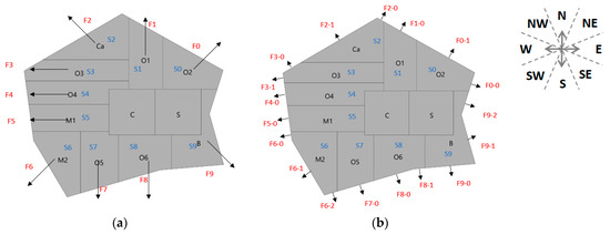
Figure 5.
An example layout illustrating the calculation of design indicators. (a) Example layout and the orientation of each room defined based on internal walls, as black arrows show; (b) Example layout and the orientation of each façade shown with black arrows. Note: O1—office-1, O2—office-2, O3—office-3, O4—office-4, O5—office-5, O6—office-6, M1—meeting-1, M2—meeting-2, Ca—canteen, B—break room, C—core, S—staircase.
In this study, the design indicators that are more relevant to façades, i.e., the façade area ratio and height-to-depth ratio, were calculated based on the façade orientation, as shown in Figure 5b. Other indicators that are also relevant to floors, i.e., the floor area ratio and ff-ratio, were calculated based on the normal of internal walls, as shown in Figure 5a. Each design indicator is explained in detail in the following subsections. Additionally, the nomenclature used in these indicators is listed in Table 4.
Table 4.
Nomenclature.
3.1. Design Indicators for the Whole Layout
The design indicators discussed in this section were calculated for the whole layout without considering the difference between functions. Taking the layout in Figure 5 as an example, the detailed calculation of these design indicators is presented hereafter.
3.1.1. Floor Area Ratio per Orientation
The floor area ratio per orientation (floor-orientation) was calculated based on room area; the orientation of each room was determined based on the orientation of internal walls, as shown in Figure 5a. Taking floor − S as an example, Office-5 and Office-6 faced South in this layout, as shown in Figure 5a. The floor − S was calculated as follows:
3.1.2. Façade Area Ratio per Orientation
The façade area ratio per orientation (façade-orientation) was calculated based on each façade segment, and the orientation of each segment was determined individually as shown in Figure 5b. Taking the calculation of facade − S as an example, Office-5, Office-6, the break room and one facade of Meeting-2 faced South. The facade − S was calculated as follows:
3.1.3. Façade Area-to-Floor Area Ratio per Orientation
The façade area-to-floor area ratio per orientation (ff-orientation) was calculated based on the ratio of each room, and its orientation was determined based on the orientation of each room as shown in Figure 5a. The calculation procedure of this indicator is as follows: firstly, the ff-ratio was calculated for each room; subsequently, the value of each room was normalised over all rooms in the same orientation by multiplying its floor area ratio, and the normalised values of all rooms in the same orientation were summed up; finally, the value of each orientation was normalised over all orientations by multiplying the ratio of the floor area of the orientation over all orientations, in order to be compared with other orientations. Taking ff − S as an example, Office-5 and Office-6 faced South in this layout, so ff − S was calculated as follows.
Step 1: Calculating the ff-ratio for each room in the South:
For office-5:
For office-6:
Step 2: Normalising the ff-ratios over all rooms in the South by multiplying their floor area ratios:
Step 3: Normalising the value for South over all orientations by multiplying the floor area ratio:
The function was simplified as follows:
3.1.4. Height-to-Depth Ratio per Orientation
The height-to-depth ratio per orientation (hd-orientation) was calculated based on the façade orientation, as shown in Figure 5b. Similar to the ff-orientation, this indicator was also normalised, with the façade area ratio as the weight factor. Taking hd − S as an example, one facade of Meeting-2, Office-5, Office-6, and one façade of the break room faced South in this layout, thus hd − S was calculated as follows:
Step 1: Calculating the height-to-depth ratio for each façade facing South.
Meeting-2 had one facade facing South:
Office-5 had one facade facing South:
Office-6 had two façades facing South:
The break room had one facade facing South:
Step 2: Normalising each ratio over all rooms in the South by multiplying the façade area ratio:
Step 3: Normalising the value for South over all orientations by multiplying the façade area ratio:
The function was simplified as follows:
3.2. Design Indicators for Each Function
The same type of indicators for the whole layout were calculated for each function in this section, and their calculation methods were similar to the ones for the layout. Therefore, the calculation of the indicators per function is presented here only with an example.
3.2.1. Floor Area Ratio per Function per Orientation
Regarding the calculation of the floor area ratio per function per orientation (floor-function-orientation), floor – office − S was used as an example, following the orientation definition shown in Figure 5a:
3.2.2. Façade Area Ratio per Function per Orientation
Regarding the calculation of the façade area ratio per function per orientation (facade-function-orientation), the calculation of facade – office − S was used as an example, following the orientation definition shown in Figure 5b:
3.2.3. Façade Area-to-Floor Area Ratio per Function per Orientation
Regarding the calculation of the façade area-to-floor area ratio per function per orientation (ff-function-orientation), the weight factor used for normalisation was calculated over the area of rooms with the same function. The calculation of ff – office − S was used as an example following the orientation definition shown in Figure 5a and it was calculated as follows:
Step 1: Calculating the ff-ratio for each office in the South. In this case, Office-5 and Office-6 faced South.
For Office-5:
For Office-6:
Step 2: Normalising the ratios over all offices in the South by multiplying the floor area ratio:
Step 3: Normalising the value for South over all offices by multiplying the floor area ratio:
The function was simplified as follows:
4. DOE and Relationship Analysis
DOE helps perform a smart exploration of the design space by changing the values of inputs in order to obtain good statistical understanding of the reasons for the changes in outputs by identifying the sources of variation. A DOE (Design of Experiment) was run in this section with the computational method shown in Section 2. Based on the DOE results, we analysed the relationship between space layout and energy demands.
4.1. DOE Algorithm and Results
As for the structure of DOE, the design variables were used as inputs; the energy demands and the design indicators shown in Section 3 were used as outputs. In addition to the energy demands of the layout, the energy demand of each function (function-energy) was also used as outputs for DOE, and it was calculated as the energy demand of all rooms with the same function per room area (kWh/m2).
In order to get the maximum information using the minimum number of samples, DOE sampling is necessary to guide the choice of samples. Uniform Latin Hypercube (ULH) [28] is a stochastic DOE algorithm, and the designs created by ULH are relatively uniformly distributed over the variable range by minimising correlations between input variables and maximising the distance between the generated designs. Thus, ULH was used for DOE sampling with 500 evaluations in this study.
Although 500 evaluations were planned for DOE, some errors occurred. These errors were mainly caused by the room area difference which was bigger than 10% and the scenario ignored for splitting layouts as shown in Section 2.2.3. In total, 448 evaluations were completed, among which 90 were feasible designs, i.e., designs that satisfied the layout area constraint. The total computational time was 210 h 18 min, around 8.8 days.
4.2. Method for Relationship Analysis
This study aims to extract the relationships between design indicators and energy demands. By comparing their relationships, the design indicator which is the most influential for the corresponding energy demand can be identified.
As for the method used for relationship analysis, since some scatter plots between design indicators and energy demands showed clear linearity, linear correlations were expected. Therefore, the following two methods were used for relationship analysis: the Pearson correlation [29] and regression analysis [30]. The Pearson correlation was used to identify the linear relationship between two variables, such as between ff-ratio and heating demand. Multivariate linear regression analysis was used to identify the relationship between several predicators (such as the heating demand of offices, heating demand of meeting rooms, heating demand of the canteen) and one response (such as the heating demand of the layout). By comparing the regression coefficients of different predicators, we could identify which predicator was more influential in the response than the others.
The Pearson correlation is a measure of linear association between two variables, with a value between −1 and 1 [31]. The value of correlation coefficient represents the strength of correlation of the two tested variables. If the absolute value is within 0.1 to 0.3, they have a low correlation; if the absolute value is within 0.3 to 0.5, they have a medium correlation; if the absolute value is within 0.6 to 1.0, they have a high correlation. In this study, we only focused on medium and high correlation, i.e., where the coefficient was higher than 0.30. Multivariate linear regression analysis requires the predicators to not have perfect collinearity, and therefore was only used in Section 4.3.2 for the relationship between the energy demand of the layout and energy demand of each function, as it was the only case among all cases in which predicators had no collinearity.
4.3. Analysis of the Relationship between Energy Demands
For the relationship between energy demands, the correlations between different demands for the layout were analysed first. Additionally, to figure out which function was influential on the variance of the energy demands of the whole layout, the relationship between the energy demand of the layout and energy demand of each function was also analysed.
4.3.1. Relationship between Different Energy Demands of the Layout
The correlation coefficients between the energy demand and the ff-ratio for the layout, resulting from Pearson correlation analysis, are shown in Table 5.
Table 5.
Correlation coefficients between energy demands and ff-ratio for the layout.
As shown in Table 5, the correlations between energy demands and ff-ratio for the layout were analysed and the following correlations were found:
- The ff-ratio for the layout had a positive correlation with the heating demand, as well as with the cooling demand: A compact building, i.e., with a low ff-ratio, helped save heating and cooling demands.
- The ff-ratio for the layout had a negative correlation with the lighting demand: More façade area, i.e., with a high ff-ratio, helped receive more daylight.
- The correlation between the heating demand and the cooling demand was positive: A building with a low heating demand was most probably compact, resulting in a low cooling demand.
- The correlation between thermal demands and the lighting demand was negative: A building with low thermal (heating and cooling) demands was most probably compact, and this resulted in a high lighting demand.
4.3.2. Relationship between Energy Demand of the Layout and Energy Demand of Each Function
Multivariate linear regression analysis was conducted regarding the relationship between energy demand of the layout and energy demand per function. The energy demands for each function (e.g., the heating demand of offices, meeting rooms, canteen, break room, core, and the staircase) were used as predicators, and the energy demand of the layout (e.g., the heating demand of the layout) was used as the response. The regression analysis was run three times for the heating demand, cooling demand and lighting demand, respectively. The method of Enter was used for each regression analysis. With the Enter method, all independent variables (i.e., the energy demands for each function) were entered in a single step [32], which meant that all variables were given equal importance in the model.
The regression coefficients and R-square values resulting from each round of analysis are shown in Table 6. The regression coefficient indicates the influence of each predicator on the response, i.e., the energy demand per function on the variance of the energy demand for the layout. By comparing the coefficients, we could identify the most influential function for the variance of the energy demand for the layout. It is clear that compared to other functions, offices had the highest influence on the energy demands of the layout, followed by meeting rooms. The reason for offices’ great influence on the energy demands of the layout was that this function had the highest requirements for lighting, heating and cooling. Additionally, compared to other functions, offices had the most rooms, followed by meeting rooms.
Table 6.
The regression coefficients resulting from three rounds of regression analysis for heating, cooling and lighting demand, respectively, between energy demand of the layout and energy demands of different functions.
4.4. Analysis of the Relationship between Energy Demands and Design Indicators for the Layout
The four types of design indicators for the whole layout, as explained in Section 3.1, were analysed for their correlations with the energy demands for the layout. Comparing the four types of design indicators, the energy demands of the layout had no clear correlation with floor-orientation, nor with façade-orientation and hd-orientation. Clear correlations were only shown between energy demands and the ff-orientation, as presented in Table 7, and their correlations are explained as follows:
Table 7.
Correlation coefficients between energy demands and ff-orientations for the layout.
- Ff-orientations had positive correlations with thermal demands: A smaller ff-orientation meant compact rooms, resulting in low heating and cooling demands.
- Ff-orientations had negative correlations with the lighting demand: If the ff-orientation was smaller, the façade area of the relevant room was smaller, resulting in less daylight. So, more electric lighting was needed as a consequence.
- Heating demand was more sensitive to ff-orientations than cooling and lighting demands: The coefficients between heating demand and ff-orientations were higher than with cooling and lighting demands. For instance, the coefficient was 0.68 between ff-SE and the heating demand, while this figure was 0.35 for the cooling demand and −0.33 for the lighting demand.
- Corners were more influential to energy demands compared to the other locations: Ff-corners had higher coefficients than other locations. For instance, ff-SE showed clearer linearity with the heating demand compared to ff-S (0.68 for ff-SE vs. 0.28 for ff-S). This is because corner rooms had a greater façade area than the other rooms, resulting in a greater influence on energy demands.
4.5. Analysis of the Relationship between Energy Demands and Design Indicators for Each Function
The four types of design indicators for each function, as explained in Section 3.2, were analysed for their correlations with the energy demands of the corresponding function. Comparing the four types of design indicators, only ff-function-orientations had clear correlations with energy demands for each function. Facade-function-orientation, floor-function-orientation and hd-function-orientation did not have such correlations. In addition, the following correlations were found:
- Compared to the other locations, corners were more influential on energy demands for each function: Corner rooms had higher coefficients than the other rooms. The reason was the same as the correlation between ff-orientations and energy demands, as explained in Section 4.4.
- Ff-function-corners had negative correlations with the lighting demand per function and positive correlations with the heating and cooling demand per function: This was for similar reasons to ff-corners, as shown in Section 4.4.
Additionally, different functions were compared regarding their coefficients between their energy demands and design indicators. One interesting characteristic was found. Offices and the canteen were used as an example. Comparing the coefficients of offices and the canteen in Table 8 and Table 9, most of the coefficients of offices were lower than the values of the canteen, such as the coefficients between ff-SE and the cooling demand (0.316 for offices vs. 0.533 for the canteen). To find out the reason for this, the correlations between the ff-ratio in NW and the heating demand were used as an example, as shown in Figure 6. Much clearer linearity was shown for the canteen (Figure 6b) compared to offices (Figure 6a). In comparison, clear linearity was shown for a single office (Figure 6c). Therefore, the reason for the lower coefficient for offices (shown in Table 8) was that offices had six rooms, while the canteen only had one room. The influence of the ff-ratio of offices was undermined by the room numbers.
Table 8.
Correlation coefficients between energy demands of offices and ff-office-orientations (ff-O-orientations).
Table 9.
Correlation coefficients between energy demands of canteen and its design indicators.
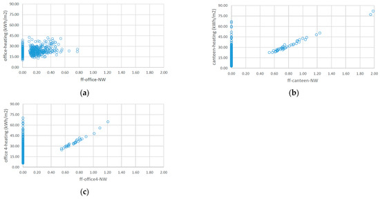
Figure 6.
Scatter charts for ff-NW and the heating demand. (a) Scatter chart of ff-office-NW and heating demand of offices; (b) Scatter chart of ff-canteen-NW and heating demand of canteen; (c) Scatter chart of ff-office4-NW and heating demand of office-4. Note: The zero ff-ratio in these figures means that in the layout, no room was located facing that specific orientation. For instance, if ff-office-NW is zero, this means that in the layout, no office was oriented NW.
4.6. Comparison between Four Types of Design Indicators
Based on the former analysis in Section 4.3, Section 4.4 and Section 4.5, ff-ratio showed a greater influence on energy demands than the other three types of design indicators. To validate this conclusion and better compare the four types of design indicators, the correlations between each design indicator for one single room and the corresponding energy demand were analysed. Taking the canteen as an example, which had one room in the layout, the correlation coefficients between all design indicators of the canteen and its energy demands are shown in Table 9.
As shown in Table 9, ff-ratio had much higher coefficients with the energy demands of the canteen than the other three types of design indicators. Taking the coefficient between the design indicators in SE (C-SE) and cooling demand as an example, the values was 0.533 for ff-ratio, while the values was 0.467 for floor area ratio, 0.046 for façade area ratio and 0.103 for height-to-depth ratio. This meant that ff-ratio had a greater influence on energy demands than the other three types of design indicators, both for each room and for the whole layout.
5. Optimisations for Minimising Energy Demands
The computational method developed in Section 2 was used for the optimisation to minimise energy demands in this section. The minimisation of annual heating, cooling and lighting demands were used as the objectives of optimisation. The algorithm used for the optimisations was pilOPT [33], a multi-strategy proprietary algorithm developed by ESTECO. This algorithm serves both global exploration and local refinement, depending on its artificial intelligence decisions based on the observed performance. Furthermore, it exploits time availability during the design evaluation to train meta-models that are used internally to define the strategy. PilOPT works well with moderate-to-heavy simulations due to its underlying artificial intelligence processes. The optimisations in this study used the autonomous mode, with which pilOPT automatically defined the number of designs to be evaluated based on the information gathered during optimisation, stopping once the Pareto frontier could not be improved any further.
Two rounds of optimisation were run in total. As shown in Section 5.1, the first round included three single-objective optimisations for minimising the heating, cooling and lighting demands, respectively. As shown in Section 5.2, the second round had one optimisation with the multi-objective of minimising heating, cooling and lighting demands together.
5.1. Single-Objective Optimisations for Minimising Each Energy Demand
Three optimisations were run with the following objectives: minimising heating demand, minimising cooling demand and minimising lighting demand, respectively. The single-objective optimisation aimed to investigate the extent to which energy demands could be saved by changing space layouts, and to find the layouts with minimum energy demands in order to validate the conclusions about the relationships identified in Section 4. The optimisation results and the layouts with minimum energy demands are presented and discussed below.
5.1.1. Results of the Optimisations
The computational time used by each optimisation is shown as follows:
- Regarding the optimisation for minimising heating demand, 297 evaluations (261 completed, 36 errors) were run, taking 106 h 56 min, around 4.4 days.
- Regarding the optimisation for minimising cooling demand, 302 evaluations (280 completed, 22 errors) were run, taking 125 h 59 min, around 5.3 days.
- Regarding the optimisation for minimising lighting demand, 438 evaluations (371 completed, 67 errors) were run, taking 192 h 24 min, around 8 days.
The reduction in each energy demand resulting from the optimisations is shown in Table 10. The reduction (%) was calculated as dividing the difference between maximum demand and minimum demand by the maximum demand. It was found that changing the function allocation, layout boundary and interior partition resulted in a reduction of up to 54% in lighting demand, 51% in heating demand and 38% in cooling demand.
Table 10.
The reduction in each energy demand resulted from single-objective optimisations.
5.1.2. Resulting Layouts with Minimum Lighting Demand
Among all layouts which were created by the optimisation for minimising the lighting demand and also satisfied the layout area constraint, the layout with minimum lighting demand (1.9 kWh/m2) is identified and shown in Figure 7. Additionally, the layout with maximum lighting demand (4.1 kWh/m2) and the layout with average lighting demand (3.0 kWh/m2) are also shown in Figure 7, in order to better analyse the characteristic of the layout with the minimum lighting demand. By comparing the three layouts, the following conclusions were drawn:
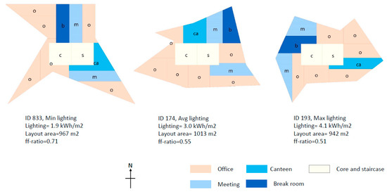
Figure 7.
The layout with minimum lighting demand, average lighting demand and maximum lighting demand, resulting from the optimisation for minimising lighting demand. Note: ID is the number of designs in the optimisation.
- The ff-ratio was relatively high in the layout with the minimum lighting demand: The ff-ratio of the layout with the minimum lighting demand was 0.71, while the ff-ratios of the other two layouts were 0.55 and 0.51, respectively. The layout with the minimum lighting demand had the largest facade area compared to the other two layouts in order to receive more daylight, resulting in a high ff-ratio. This was similar to the conclusions of Section 4.3.1.
- Corner rooms had a larger façade area than the other rooms in the layout with the minimum lighting demand: In the layout with the minimum lighting demand, corner rooms had much larger façade areas than the other rooms, i.e., corner rooms had high ff-ratios. This is similar to the conclusions about the ff-orientation and energy demands in Section 4.4.
- Offices were located in corner rooms in the layout with the minimum lighting demand: In the layout with the minimum lighting demand, all corner rooms were used as offices, which had the highest lighting requirement than the other functions. Locating more important functions in corner rooms helped save lighting demand, which is similar to the conclusions of Section 4.3.2.
- Rooms in the North were more compact than the other orientations in the layout with the minimum lighting demand: This is different from what Section 4.4 shows, i.e., the negative correlation between ff-N and lighting demand. The reason for the difference is that in order to reach a high ff-ratio for the layout while also keeping the same layout area, the less important orientation (N) was compromised in order to achieve better performance in the other, more important orientations.
5.1.3. Resulting Layouts with Minimum Heating Demand
Among all layouts which were generated from the optimisation for minimising heating demand and also satisfied the layout area constraint, the layout with minimum heating demand (13.8 kWh/m2) was identified and shown in Figure 8. Additionally, the layout with maximum heating demand (28.1 kWh/m2) and the layout with average heating demand (21 kWh/m2) are shown in Figure 8. By comparing the three layouts, it was found that the ff-ratio of the layout with the minimum heating demand was relatively low. The ff-ratio of the layout with the minimum heating demand was 0.4, while the ff-ratios of the other two layouts were 0.5 and 0.7, respectively. A smaller ff-ratio resulted in a smaller façade area, which caused a smaller heat loss through the façade. This is similar to the conclusions of Section 4.3.1.
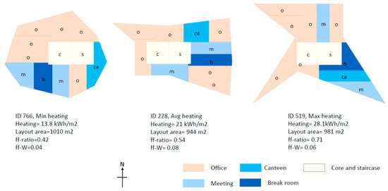
Figure 8.
The layout with minimum heating demand, average heating demand and maximum heating demand, resulting from the optimisation for minimising heating demand.
There is a clear characteristic of the layout with the minimum heating demand: no room was east-oriented, for which the room orientations were defined based on the normal of internal walls, as Figure 5a shows. In order to find out the reason for this characteristic, the layouts that had no room orienting West, and which also had a low ff-ratio (lower than 0.46 for a low heating demand), were identified and are shown in Figure 9. The three layouts in Figure 9 were compared with the layout with the minimum heating demand (ID 766) shown in Figure 8. The east-oriented rooms in Figure 9 (with an ff-E of 0.06) were wider than the west-oriented rooms in ID 766 (with an ff-W of 0.04). The wider room resulted in a higher heating demand for layouts in Figure 9 than the layout of ID 766.
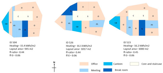
Figure 9.
Layouts with no room orienting West, resulting from the optimisation for minimising heating demand. Note: The room orientations were defined based on the normal of internal walls.
The reason for the characteristic of the layout with minimum heating demand is the manner in which the layouts were generated, as shown in Figure 3d. The starting line to split the layout (Line-0) had a fixed location for every layout, and the first splitting line (Line-1) was always orientated towards the North. Therefore, the NE-corner room was always attached to the staircase. This resulted in less freedom for the locations of east-oriented rooms compared to west-oriented rooms. Thus, the layout with no room orientating East helped achieve a lower heating demand in this case, implying that the constraint of the location of internal walls results in the specific preference of room locations when optimising the layouts for minimising the heating demand.
5.1.4. Resulting Layouts with Minimum Cooling Demand
Among all layouts which were generated from the optimisation for minimising cooling demand and also satisfied the layout area constraint, the layout with minimum cooling demand (3.4 kWh/m2) was found and shown in Figure 10, as well as the layout with maximum cooling demand (6.7 kWh/m2) and the layout with average cooling demand (5.0 kWh/m2). By comparing the three layouts, the following conclusions were drawn:
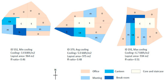
Figure 10.
The layout with minimum cooling demand, average cooling demand and maximum cooling demand, resulting from the optimisation for minimising cooling demand.
- The ff-ratio of the layout with the minimum cooling demand was relatively low: A low ff-ratio also helped reduce the façade area and heat losses through the façade well. The situation is similar to the layout with minimum heating demand.
- More rooms were orientated towards the North, East and West than the South in the layout with the minimum cooling demand: In this layout, only one room was south-oriented, and it was used as a break room—the function with the lowest requirement for cooling. Although a low ff-ratio helped reduce the cooling demand for all orientations, a compromise was needed to accommodate all rooms within one layout. Locating fewe rooms in the South helped reduce the cooling demand of the whole layout.
5.2. Multi-Objective Optimisation for Minimising All Energy Demands
The optimisation with the multi-objective for minimising heating, cooling and lighting demands was run and is shown in this subsection. This optimisation aimed to illustrate how to apply the computational method developed in this study with multiple objectives and to compare it with the single-objective optimisations. In total, 1447 evaluations (1393 completed, 54 failed) were run, among which 925 designs satisfied the layout area constraint, i.e., the feasible designs. The total computational time used for the optimisation was 598 h and 46 min, around 25 days. All feasible designs of the optimisation are shown in a 3D chart with the heating demand (kWh/m2) as x axis, the cooling demand (kWh/m2) as y axis and the lighting demand (kWh/m2) as z axis in Figure 11.
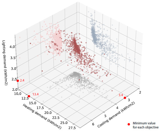
Figure 11.
3D chart for feasible designs of the multi-objective.
As shown in Figure 11, the resulting minimum lighting, heating and cooling demands from the multi-objective optimisation were 2.4 kWh/m2, 13.4 kWh/m2 and 3.4 kWh/m2, respectively. Comparing the resulting minimum demands from the single-objective optimisations as shown in Table 10, the minimum lighting demand resulting from the multi-objective optimisation was much higher than the minimum lighting demand resulted from the single-objective optimisation. The multi-objective optimisation may need a longer time to find the similar value to what was found from the single-objective optimisation. The reason is that the correlation between the heating demand and cooling demand was positive, while the correlation between the lighting demand and the thermal demands (heating and cooling) was negative. For instance, a compact layout with a low ff-ratio resulted in low heating and cooling demands but a high lighting demand. It is plausible that the negative correlation between the lighting demand and the thermal demands made the multi-objective optimisation require a much longer time to find the minimum lighting demand than heating and cooling demands.
Regarding the resulting layouts from the multi-objective optimisation, the best solution for minimising all energy demands could not be directly found, as the three energy demands were conflicting, as explained in Section 4.3.1. However, designers can choose the best solution based on their own preference or the specific requirements of the project, by defining their own criteria—such as different weighting factors—for choosing between different energy demands. For instance, if the thermal demands of the project are dominant, designers can give a greater weighting factor to thermal demands and a smaller weighting factor to the lighting demand. In this way, the best solution can be identified.
6. Conclusions, Recommendations and Limitations
With the goal of studying the relationship between space layout variations and energy performance, this study developed a computational method for generating a space layout and evaluating the energy performance of the layouts generated for a temperate climate (Amsterdam). Four types of design indicators were proposed to characterise space layouts, both for the whole layout and for each function. The design of experiments method (DOE) was run using the computation method with energy demands as outputs. Based on the DOE results, the relationships between design indicators of space layout and energy demands were identified and compared. Additionally, two rounds of optimisation for minimising heating, cooling and lighting demands were run, i.e., three single-objective optimisations and one multi-objective optimisation. Based on each single-objective optimisation, the resulting layouts with the minimum, maximum and average energy demands were found and compared. Moreover, the results of the multi-objective optimisation were compared with the single-objective optimisations.
6.1. Conclusions
Overall, this study shows that designing space layouts helps to reduce energy demands for heating, cooling and lighting, and as a consequence helps to reduce carbon emissions in the building sector. Thus, designers should consider reducing energy consumption earlier in the whole architecture design phase, particularly in the stage of space layout design. However, it is difficult to design space layout in a manual way, as the design variables of space layout are difficult to control manually and different design variables complexly influence the building energy performance. The optimisation method is necessary to obtain an energy-efficient space layout. This study makes a reference for researchers and designers on how to optimise a space layout design with improved energy performance. Additionally, more conclusions were drawn regarding the relationship between the design indicators of space layout and energy demands, as well as the optimisation results.
Regarding the relationships between design indicators and energy demands, the following conclusions were drawn:
- i.
- Comparing the four types of design indicators, façade area-to-floor area ratio (ff-ratio) showed a stronger correlation with energy demands than façade area ratio, floor area ratio and height-to-depth ratio, as explained in Section 4.6;
- ii.
- Comparing different locations within the layout, the ff-ratios of corner rooms showed stronger correlations with energy demands than the other locations, as explained in Section 4.4 and Section 4.5;
- iii.
- Comparing different functions defined in this study, the location of offices showed a stronger correlation with the energy demands for the layout than the other functions, followed by meeting rooms, as explained in Section 4.3.2.
Regarding the optimisation results, the following conclusions were drawn:
- i.
- Changing the function allocation, layout boundary and interior partition resulted in a reduction of 54% in lighting demand, 51% in heating demand and 38% in cooling demand, as shown in Section 5.1.1;
- ii.
- The multi-objective optimisation needed a longer time to find the layout with the similar value of minimum lighting demand to the single-objective optimisation, as the thermal demands had negative correlations with the lighting demand;
- iii.
- The way in which layout variants were generated could result in a specific characteristic among the layouts with the minimum energy demands. As shown in Section 5.1.3, the layouts with the minimum heating demand had no east-oriented room. As explained previously, this situation was caused by the way in which layout variants were generated.
6.2. Recommendations
Based on the results and conclusions drawn in this study, the following recommendations were made, both for designing energy-efficient space layouts and for future academic research.
6.2.1. How to Design an Energy-Efficient Space Layout
In order to help design an energy-efficient space layout, the conclusions were interpreted to the following recommendations:
- i.
- Designers can design a space layout by changing the ff-ratio, which helps find a layout with low energy demands quickly. For example, designing a building with a lower ff-ratio, i.e., smaller façade area and greater floor area, would result in a lower heating demand in the temperate climate.
- ii.
- Designers should pay attention to internal partitions in order to reduce energy demands in building design. In general, internal partitions are considered at a quite late design phase. However, the internal partition determines the ff-ratio for each room, and this study proves that this ratio is highly influential towards building energy demands.
- iii.
- Locating important functions in corner rooms helps find the layout with smaller lighting demand in a temperate climate.
- iv.
- The computational method is necessary to design a space layout for minimising energy demands, since the design variables of space layouts cannot be easily changed manually to satisfy the functional requirements (such as room area) and energy performance cannot be predicted directly.
6.2.2. Recommendations for Future Research
For future research, the following recommendations were given regarding the generation of space layout, assessment of energy performance and optimisation of space layout design for minimising energy demands.
Different methods of generating space layout result in different characteristics of layouts with minimum energy demands. The following recommendations were made regarding the method of space layout generation:
- i.
- Adding more control points to change the layout boundary: Eight control points were used in this study, while more control points would result in more freedom in the layout boundary. However, more control points mean more design variables, which would require more computational time.
- ii.
- Improving the applicability of the generated space layouts: Some of the generated layouts in this study may be inapplicable in practice, such as the triangle layout. Future research should add more constraints to the generation of space layout shown in this study, in order to avoid the possibility of triangle layouts and rooms. For instance, researchers can develop a constraint for limiting the compactness of the layout boundary, i.e., keeping the façade area-to-floor area ratio as a relative low value.
- iii.
- Adding variation in room height: The difference in height between different rooms of one layout would cause a greater difference in energy demands. For future research, room height could be considered as one extra design variable in the optimisation, and its relationship with energy performance could be tested.
- iv.
- Separating the locations of the core and staircase: the core and staircase were adjacent to each other in this study, but they can also be located in opposite orientations in practice.
Regarding the assessment of energy performance, the following recommendations were made:
- i.
- Testing more climates, such as cold and tropical climates: This study only tested a temperate climate. Different climates have different dominant energy demands, such as heating demand in a cold climate and cooling demand in a tropical climate. It is also expected that the same function in different climates would have different preferences for location, orientation and ff-ratio, due to a differing course of the sun.
- ii.
- Testing other design variables for their influence on the effect of space layout on energy demands, such as WWR, thermal mass, façade properties (thermal properties of the façade, optical property of glazing and shading devices), shading control type and set points for heating, cooling and lighting.
- iii.
- Testing more functions with a greater difference in comfort requirements: It is the difference in the thermal and visual comfort requirements between functions that makes changing function allocations meaningful for reducing energy demands. A greater difference in comfort requirements between functions results in a greater influence of space layout (e.g., function allocation) on energy demands.
Regarding the optimisation of space layout design for minimising energy demands, the following recommendations were made:
- i.
- Reducing computational time for optimisation: With four computers run in parallel for computation in this study, the multi-objective optimisation still took around 25 days. Long computational time is the primary obstacle for applying the optimisation method of space layout design to minimise energy demands in practice. More methods are needed to reduce computational time.
- ii.
- Different methods for space layout optimisation: Generally, two methods for the optimisation of space layout are used, concerning its design variables. One is optimising the layout boundary first and then optimising the other design variables of the space layout, e.g., function allocation; the other method is optimising all design variables together, as this study did. It is difficult to tell which one is better, therefore it is necessary to compare the two methods regarding their computational time and resulting reduction in energy demands.
6.3. Limitations
This paper aims to identify the relationship between space layout and energy performance and gain theoretic understanding of the subject. Therefore, the computational method developed in Section 2.2 generated schematic space layouts with the goal of testing large set of variations featuring geometric properties relevant to energy performance. As a result, the layouts were not generated with the focus on functionality (such as space connection, space adjacency, orientation preference and room dimensions) and direct applicability in architectural practice. The generated layouts also include configurations that can be quite impractical, such as ID 833 in Figure 7. In order to apply the generated schematic layouts in practice, designers need to select the generated layouts based on functional requirements and elaborate them from schematic configurations to proper architectural layouts. Alternatively, designers need to modify this computational method and integrate it with the functional requirements of space layout.
Considering the case of adding functional requirements to the generation method of space layout in Section 2.2, the resulting layout configurations would be different from the layouts shown in this paper. For instance, a layout configuration similar to ID 833 in Figure 7 would not be considered in this case, and by analysing the layouts created from the above case, the resulting relationship between space layout and energy performance would be different from what is presented in Section 4. This is because the threshold of the variation of energy demands would be smaller than what is shown in this paper, as well as the variation in design indicators, such as façade area-to-floor area ratio. In this case, it is difficult to tell whether there are still the same correlations between the design indicators of space layout and energy demand as shown in this paper. More studies are needed.
Author Contributions
Conceptualization, T.D. and M.T.; Data curation, T.D. and M.T.; Formal analysis, T.D.; Investigation, T.D.; Methodology, T.D., M.T. and F.D.L.; Software, T.D. and F.D.L.; Supervision, M.T., S.J. and A.v.d.D.; Validation, S.J.; Writing—original draft, T.D.; Writing—review & editing, M.T., S.J., A.v.d.D. and F.D.L. All authors have read and agreed to the published version of the manuscript.
Funding
The work of Francesco De Luca was supported by European Regional Development Fund 2014-2020.4.01.15-0016 and European Commission 856602.
Institutional Review Board Statement
Not applicable.
Informed Consent Statement
Not applicable.
Acknowledgments
We want to show our sincere thanks to Gabriele Degrassi and other experts at ESTECO for their guidance on the use of modeFRONTIER, Aytac Balci from Delft University of Technology for his help in coordinating the four computers at the TU Delft Renderfarm, as well as Shengzhi Xu for his generous help in the discussion on coding during the generation of space layouts.
Conflicts of Interest
The authors declare no conflict of interest.
References
- Lobos, D.; Donath, D. The problem of space layout in architecture: A survey and reflections. Arquitetura Rev. 2010, 6, 136–161. [Google Scholar] [CrossRef] [Green Version]
- Musau, F.; Steemers, K. Space Planning and Energy Efficiency in Office Buildings: The Role of Spatial and Temporal Diversity. Archit. Sci. Rev. 2008, 51, 133–145. [Google Scholar] [CrossRef]
- Dino, I.G.; Üçoluk, G. Multiobjective Design Optimization of Building Space Layout, Energy, and Daylighting Performance. J. Comput. Civ. Eng. 2017, 31, 04017025. [Google Scholar] [CrossRef]
- Zhang, S.; Ma, M.; Li, K.; Ma, Z.; Feng, W.; Cai, W. Historical carbon abatement in the commercial building operation: China versus the US. Energy Econ. 2022, 105, 105712. [Google Scholar] [CrossRef]
- Chen, H.; Wang, L.; Chen, W. Modeling on building sector’s carbon mitigation in China to achieve the 1.5 °C climate target. Energy Effic. 2019, 12, 483–496. [Google Scholar] [CrossRef]
- Ekici, B.; Cubukcuoglu, C.; Turrin, M.; Sariyildiz, I.S. Performative computational architecture using swarm and evolutionary optimisation: A review. Build. Environ. 2019, 147, 356–371. [Google Scholar] [CrossRef]
- Evins, R. A review of computational optimisation methods applied to sustainable building design. Renew. Sustain. Energy Rev. 2013, 22, 230–245. [Google Scholar] [CrossRef]
- Rodrigues, E.; Gaspar, A.R.; Gomes, Á. Automated approach for design generation and thermal assessment of alternative floor plans. Energy Build. 2014, 81, 170–181. [Google Scholar] [CrossRef]
- Du, T.; Turrin, M.; Jansen, S.; Van Den Dobbelsteen, A.; Fang, J. Gaps and requirements for automatic generation of space layouts with optimised energy performance. Autom. Constr. 2020, 116, 103132. [Google Scholar] [CrossRef]
- Tiantian, D. Space Layout and Energy Performance: Parametric Optimisation of Space Layout for the Energy Performance of Office Buildings; A+BE|Architecture and the Built Environment: Delft, The Netherlands, 2021; ISBN 9789463664356. [Google Scholar]
- Cavazzuti, M. Optimization Methods: From Theory to Design; Springer: Berlin/Heidelberg, Germany, 2012; ISBN 9783642311864. [Google Scholar]
- Grasshopper Algorithmic Modeling for Rhino. Available online: https://www.grasshopper3d.com/ (accessed on 11 October 2018).
- Esteco modeFRONTIER. Design Better Products Faster. Available online: https://www.esteco.com/modefrontier (accessed on 18 August 2020).
- Lee, H.Y.; Yang, I.T.; Lin, Y.C. Laying out the occupant flows in public buildings for operating efficiency. Build. Environ. 2012, 51, 231–242. [Google Scholar] [CrossRef]
- Ladybug Tools. Available online: https://www.grasshopper3d.com/group/ladybug (accessed on 11 October 2018).
- Shading Module: Engineering Reference-EnergyPlus. Available online: https://bigladdersoftware.com/epx/docs/8-0/engineering-reference/page-034.html#solar-distribution (accessed on 9 August 2020).
- Daysim. Available online: http://daysim.ning.com/ (accessed on 11 October 2018).
- EnergyPlus EnergyPlus. Available online: https://energyplus.net/ (accessed on 29 January 2019).
- Ramos, G.; Ghisi, E. Analysis of daylight calculated using the EnergyPlus programme. Renew. Sustain. Energy Rev. 2010, 14, 1948–1958. [Google Scholar] [CrossRef]
- Du, T.; Jansen, S.; Turrin, M.; van den Dobbelsteen, A. Effect of space layouts on the energy performance of office buildings in three climates. J. Build. Eng. 2021, 39, 102198. [Google Scholar] [CrossRef]
- Itard, L. Energy in the Built Environment. In Sustainable Urban Environments; van Bueren, E., van Bohemen, H., Itard, L., Visscher, H., Eds.; Springer: Dordrecht, The Netherlands, 2012; pp. 113–175. ISBN 9789400712942. [Google Scholar]
- NEN-16798-1; Energy Performance of Buildings-Part 1: Indoor Environmental Input Parameters for Design and Assessment of Energy Performance of Buildings Addressing Indoor Air Quality, Thermal Environment, Lighting and Acoustics-Module M1-6. Netherlands Standardization Institute: Delft, The Netherlands, 2015; pp. 42–43.
- Deru, M.; Field, K.; Studer, D.; Benne, K.; Griffith, B.; Torcellini, P.; Liu, B.; Halverson, M.; Winiarski, D.; Rosenberg, M.; et al. U.S. Department of Energy Commercial Reference Building Models of the National Building Stock; Office of Energy Efficiency & Renewable Energy: Washington, DC, USA, 2011.
- Setting Rendering Options. Available online: https://floyd.lbl.gov/radiance/refer/Notes/rpict_options.html (accessed on 29 July 2019).
- Aksoy, U.T.; Inalli, M. Impacts of some building passive design parameters on heating demand for a cold region. Build. Environ. 2006, 41, 1742–1754. [Google Scholar] [CrossRef]
- Bostancioǧlu, E. Effect of building shape on a residential building’s construction, energy and life cycle costs. Archit. Sci. Rev. 2010, 53, 441–467. [Google Scholar] [CrossRef]
- Gonzalo, R.; Habermann, K.J. Energy-Efficient Architecture: Basics for Planning and Construction. Available online: https://books.google.nl/books?hl=zh-CN&lr=&id=6bhB8Tt3T4EC&oi=fnd&pg=PA5&dq=Energy-Efficient+Architec-+ture:+Basics+for+Planning+and+Construction.&ots=JrfkqWu8zL&sig=cczxCE7I16WtJ6WwE1NXO4WuMK0&redir_esc=y#v=onepage&q=Energy-Efficient Architec-ture%3A Ba (accessed on 30 October 2020).
- McKay, M.D.; Beckman, R.J.; Conover, W.J. A comparison of three methods for selecting values of input variables in the analysis of output from a computer code. Technometrics 2000, 42, 55–61. [Google Scholar] [CrossRef]
- Benesty, J.; Chen, J.; Huang, Y.; Cohen, I. Pearson Correlation Coefficient. In Noise Reduction in Speech Processing; Springer: Berlin/Heidelberg, Germany, 2009; Volume 2, pp. 1–4. ISBN 9783642002960. [Google Scholar]
- Field, A. Discovering Statistics Using SPSS; SAGE Publications: London, UK, 2008; Volume 622, ISBN 978-1-84787-906-6. [Google Scholar]
- Statistics Solutions Correlation (Pearson, Kendall, Spearman)-Statistics Solutions. Available online: https://www.statisticssolutions.com/correlation-pearson-kendall-spearman/ (accessed on 6 January 2021).
- IBM. IBM SPSS Regression 22. 2011. Available online: www.cc.uoa.gr/fileadmin/cc.uoa.gr/uploads/files/manuals/SPSS22/IBM_SPSS_Regression.pdf (accessed on 6 June 2021).
- Optimization Algorithms. Design Optimization. Available online: https://www.esteco.com/technology/optimization-algorithms (accessed on 7 January 2021).
Publisher’s Note: MDPI stays neutral with regard to jurisdictional claims in published maps and institutional affiliations. |
© 2022 by the authors. Licensee MDPI, Basel, Switzerland. This article is an open access article distributed under the terms and conditions of the Creative Commons Attribution (CC BY) license (https://creativecommons.org/licenses/by/4.0/).