Digitalize the Twin: A Method for Calibration of Reference Data for Transfer Real-World Test Drives into Simulation

Abstract

In the course of the development of automated driving, there has been increasing interest in obtaining ground truth information from sensor recordings and transferring road traffic scenarios to simulations. The quality of the “ground truth” annotation is dictated by its accuracy. This paper presents a method for calibrating the accuracy of ground truth in practical applications in the automotive context. With an exemplary measurement device, we show that the proclaimed accuracy of the device is not always reached. However, test repetitions show deviations, resulting in non-uniform reliability and limited trustworthiness of the reference measurement. A similar result can be observed when reproducing the trajectory in the simulation environment: the exact reproduction of the driven trajectory does not always succeed in the simulation environment shown as an example because deviations occur. This is particularly relevant for making sensor-specific features such as material reflectivities for lidar and radar quantifiable in dynamic cases.

1. Introduction

“Ground truth (GT) data was obtained using an real time kinematic (RTK)-based global navigation satellite system (GNSS) device and provides accuracy of up to ±3 cm”. Such statements are often found in research articles to justify the quality of reference data accompanying data acquisition for various tasks [1,2]. In the automotive context, RTK-aided GNSS is widely used for obtaining positions. There is no doubt that RTK-based GNSS methods can achieve accuracies in the cm range. However, this applies only to the position determination of the antenna and under favorable operating conditions of the GNSS receiver. If one is, however, interested in the position information of another reference point, e.g., the center of the vehicle’s rear axle, the translational offsets between the antenna and the respective point must be determined very precisely. In complex geometries such as vehicles, further aids are needed for this. Uncertainties in the determination of these offsets can be hardly avoided. For this reason, it is unclear whether the specified precision of the device can also be achieved in its installed state.

In this work, we address the issue of the trustworthiness of reference data obtained with GNSS devices. We aim to refine the notion of GT in the context of environmental perception with different sensor modalities. It must be ensured that the reference measurement shows higher credibility against other sensors used, e.g., lidar or radar sensors. To determine this, reference measurements are required to determine the credibility of the reference, called the “super-reference”. 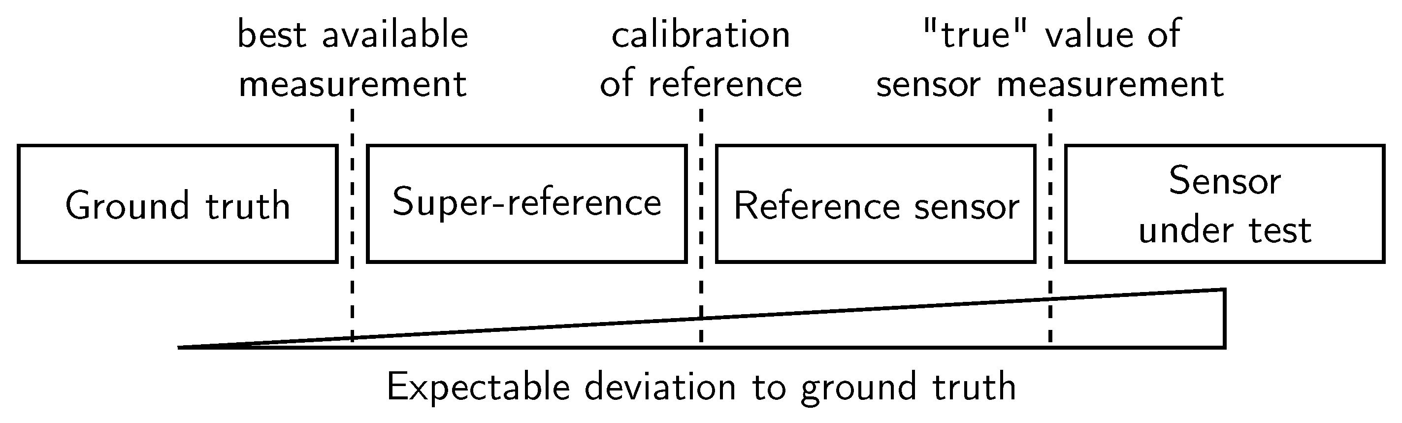Figure 1 contextualizes the aforementioned term “super-reference” in comparison to GT and a reference sensor.

The GT can only be measured with finite accuracy, which we call the super-reference. Thereby, GT is only approximated by the super-reference, leaving a minor deviation to GT. A super-reference is typically only available in limited and controllable circumstances. A reference sensor, however, is optimized for the practical application at the cost of potentially higher GT deviation. To achieve higher trustworthiness in the accuracy of the reference, a super-reference is used for its calibration. Ultimately, when validating sensors, it is of interest to determine measurement uncertainties, which result from the difference between sensor and reference measurement.

The main interest of this article lies in increasing the trustworthiness in reference data, which enables the reenacting of real-world test drives in virtual environments. This is of particular importance in the development and validation of sensor models for the virtual validation of automated driving (AD), as reference data are required. The basic idea of transferring test drives to simulation is admittedly not new. However, our paper specifically deals with the calibration process of positioning measuring devices and discusses the achievable accuracy.

This paper is structured as follows. First, we discuss the need for the careful calibration of measurement devices that are used for collecting reference data. Next, an overview of previous research on obtaining GT data and sensor principles employed for this purpose is presented. We present stationary and dynamic calibration experiments, which serve as a reference and are thereby eligible for the calibration of measurement devices. In the practical application of our experiments, we show that the proclaimed accuracy of the positioning devices is not always met. Finally, we show the achievable precision when reenacting a real-world test drive in two simulation environments. The source code for creating scenarios with real driven trajectories based on GNSS measurements is made available.

2. A Motivational Example: Can We Trust Our Reference?

After data collection with sensors in real-world scenarios, faithful reenacting of the driven scenario in simulation is tedious, but of high interest for virtual validation aspects. There are various types of measurement phenomena that are inherent in the sensor measurement principle and can manifest as measurement artefacts. These can cause deviations between the obtained measurement result and GT. A simple yet illustrative example is the limited resolution of the (discrete) distance measurement with radar and lidar sensors, which causes quantization errors in the determination of the (continuous) distance to an object. For this reason, reference sensors are needed that are capable of measuring the movement and position of vehicles with high accuracy, precision, and reliability.

Even for simple scenarios, such as a follow-up drive with an Adaptive Cruise Control (ACC) system, one can observe non-stationary behavior when inspecting the movements of the vehicles in close detail, although the vehicle movements were subjectively perceived by the occupants as stationary. If the movement of the vehicle in front is now recorded by a sensor, further sensor-specific uncertainties are superimposed on its perception.

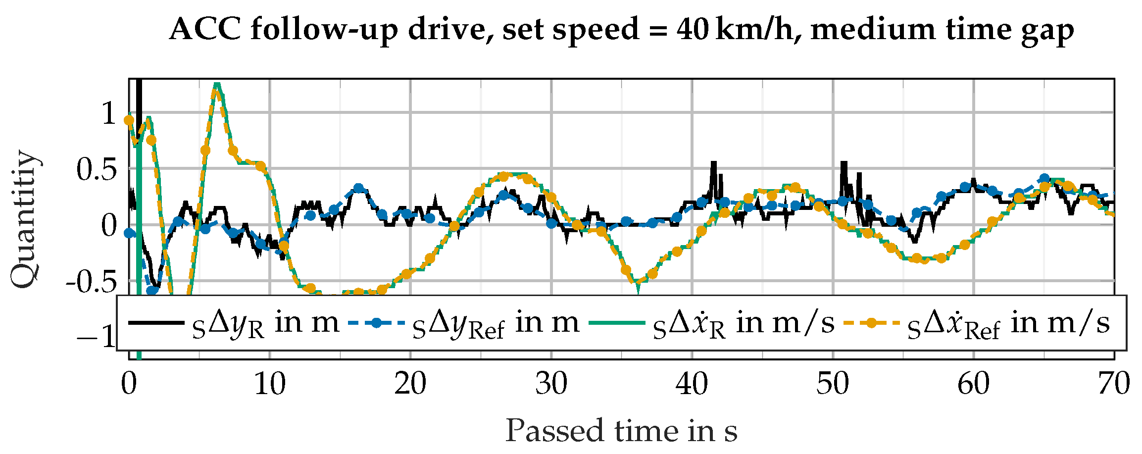
Figure 2 shows an example of a measurement record of an ACC drive run at 40 km/h with a medium time gap to the front vehicle. The measured variables used for the ACC function are read out from the radar sensor, which supplies the object information for the ACC system, via the vehicle Controller Area Network (CAN).

Several aspects emerge from the measurement record shown in the figure: the relative longitudinal velocity ${}_{\mathrm{S}}\Delta \dot{x}$ shows a variation bandwidth of $\pm 0.5$ m/s, which is around one order of magnitude above the velocity resolution of automotive radar sensors. In the lateral direction, i.e., ${}_{\mathrm{S}}\Delta y$, the object fluctuates within its lane at around ±0.2 m, which can hardly be noticed with visual inspection by a human driver. The object reported by the used radar sensor shows the pronounced discretization of the lateral measurement. The direct transfer of the radars’ measured variables into the simulation would lead to sudden, physically implausible jumps in an object’s trajectory. Although the radial velocity of objects is measured by the radar with high precision, the discretization by the sensor used in this example makes post-processing necessary in order to obtain a feasible motion profile.

There is reasonable hope that high-accuracy motion analyzers, which combine GNSS position measurements as well as accelerations and angular rates captured by inertial measurement unit (IMU) sensors, can be used to capture the motion of agents with high precision. An exemplary device is the GeneSys Automotive Dynamic Motion Analyzer (ADMA) or the RT device series by OXTS. The corresponding measurements of such a device are also shown in Figure 2 and denoted by “Ref”. However, the question remains as to the actual accuracy of measuring motion and transferring the motion to the simulation. The central question of this paper is therefore as follows: How much accuracy does a reference measurement system really provide and how does one perform its calibration?

3. Related Work

Real-world traffic is a suitable data source for developing and testing automated driving functions because it is highly diverse and has random characteristics. Moreover, regarding simulation aspects, real-world data offer the highest possible quality for the validation of simulation models. Consequently, there are several previously reported approaches to transfer a real-world test drive into the simulation.

Roughly speaking, two categories can be found. These are, on the one hand, object list-based approaches. Here, the object list from sensors or a fused sensor cluster is taken as the starting point for scenario reconstruction. The goal of this method is to prepare real data for a scenario-based testing approach in the simulation. Regarding the study of absolute accuracy, previous work in the field of reference sensing deals with obtaining the accuracy that is achievable with contemporary automotive grade perception sensors.

3.1. Object List-Based Approach

In the literature, there are approaches known in which the object lists of the sensors are used to transfer the recorded scenario into a simulation. These methods aim to extract a concrete scenario from the measurement data in the sense of scenario-based testing. Logical scenarios can be abstracted from this. A typical pipeline consumes sensor data (e.g., object lists, point clouds, etc.) and compiles a standardized scenario description using the OpenScenario/OpenDrive language format. A typical example is the framework proposed by Wagner et al. that relies on lidar sensors [3]. It is capable of sensing road objects as well as road semantics (e.g., road geometry, lane markings, etc.). There are also a number of commercial suppliers in this field that compile scenario data from sensor readings, such as [4,5].

These methods require a comprehensive object list as well as additional sensor data to facilitate the inference of the road properties or street layout. This prerequisite is not fulfilled in many everyday traffic situations, such as the occurrence of occlusions, or the cutting in/out of objects. Object detection is generally not reliable in such moments. This constraints can be gradually resolved by manual annotations of sensor data. There are no uniform quality standards, to the best of our knowledge, for the required accuracy of such methods. Based on the published information about these procedures, there is an impression that a visual inspection is performed by experts or the test engineers.

Services that provide so-called GT information for the annotation of sensor data (lidar point cloud, camera images), such as [6,7], are not within the scope of this paper because no reference data are used for this purpose. Instead, recorded sensor data, which may be calibrated extrinsically to each other when multiple sensor modalities are used, are annotated in a manual or (semi-)automated fashion.

3.2. Reference Sensors

With the help of reference sensors (e.g., high-precision GNSS measurement technology or laser scanners), the position of traffic participants can be obtained within the respective measurement accuracy. Data sets such as KITTI, nuScenes, WaymoOpen, etc., therefore provide GT information of traffic participants obtained from an automotive-grade laser scanner mounted on the roof of the ego vehicle. This approach provides useful results for annotating bounding boxes such as those used for labeling in machine learning methods. Minor inaccuracies in the labeling, so-called label noise, can even increase the robustness of the learning algorithm under certain circumstances. In order to use bounding boxes that are labeled in this way as a reference when transferring the scenario to the simulation, a specification of the accuracy over several time steps is required. This is not given in most data sets. The suitability of automotive-grade lidar sensors was investigated in a paper by Schalling et al. [8]. However, the limitations of lidar sensors with respect to the factors influencing their measurement result prevent their justification as GT sensors.

Thorough research on referencing the reference system (“super-referencing”) has been presented by Brahmi [9]. His focus is on the evaluation of object-based advanced driver assistance system (ADAS) systems. The basic ideas presented in his thesis can essentially be applied to the problem of this paper, namely the transfer of a real test drive to a simulation.

In a paper by Steinhard, the suitability of a lidar sensor system for GT determination is investigated [10]. As with Brahmi, a high-precision laser scanner with sub-mm resolution serves as a super-reference.

3.3. Gaps in State of the Art

The determination of GT is mostly done via RTK-based GNSS or high-precision lidar sensors with mm-scale resolution e.g., Leica D5. In this context, however, there is no verification that the proclaimed accuracy is actually met under all circumstances. Previous experiments, such as the work from Brahmi [9], have indeed identified the need for a calibration procedure with reference sensors. What remains unresolved so far is to study the fidelity of “GT” in dynamic cases, as well as the stationary analysis of the yaw angle between two reference systems, which is of the utmost interest in reflectivity studies and signal drift.

The digitalizing of a test run relies on the position accuracy of the RTK-based GNSS device. However, it lacks the discussion of whether the proclaimed accuracy is maintained during dynamic situations. Modern lidar and high-resolution radar sensors have distance resolutions in the cm range. If sensor models are to be validated, high demands are therefore made on the accuracy of the trajectory reproduction in the simulation.

4. Calibration Aspects: The Need for a Super-Reference

At this point, a discussion of the term “GT” in the context of automotive simulation is needed to obtain a common understanding of it. It is often used to describe the true state of an object, and potentially also the future state, e.g., in terms of planned actions. Thus, there is a state that can be estimated or measured. Its true value is called GT. It is initially irrelevant how GT is determined. The only relevant aspect is that the GT value serves as a reference against other methods for determining a certain value (measurement, estimation). Especially in the field of virtual environments, which consider 3D representations of objects, the term can be used in a broader sense: it covers material assignments, reflectively properties, as well as geometry detailing, and others.

When a “GT” is obtained with a prospective device, the resulting deviations can be conceptualized in terms of “accuracy” and “precision”. The term “accuracy” is defined as “the degree to which the result of a measurement or calculation matches the correct value or a standard” [11]. Moreover, the term “precision” is defined as “the quality of being exact, accurate and careful” [12].

GT can hardly claim to be completely accurate. It represents rather a value that can be faithfully measured to the best of one’s knowledge and belief, as well as up to the accuracy of the measurement equipment used. Prominent examples are object states, such as its longitudinal and lateral positions, as well as the object’s orientation. Measurement errors of all kinds, as they are present in all measuring instruments, mean that GT can basically only be obtained with finite accuracy. Nevertheless, the measurement data obtained using the highest-precision device are considered to be a GT measurement. Consequently, a GT to the “GT” is needed. Thus, for verification of the reference sensor, a more accurate reference is needed, the so-called “super-reference”. We define the term “super-reference” as follows:

“Comparing the result $\xi$ obtained by device $\mathcal{A}$ to that of device $\mathcal{B}$. The underlying measurement principle of $\mathcal{B}$ is fundamentally different to $\mathcal{A}$, i.e., $\mathcal{B}$ is invariant to error sources of $\mathcal{A}$. Measuring $\xi$ by means of $\mathcal{B}$ is characterized by high fidelity, accuracy, repeatability, and intuition. $\mathcal{B}$ is thereby seen as a super-reference for obtaining $\xi$”.

In order to distinguish the term “super-reference” from the calibration of a measuring device, the definition of calibration is considered. Calibration is defined as “to mark units of measurement on an instrument so that it can be used for measuring something accurately” [13]. Therefore, the usability of a measuring device for determining the “GT” is qualified by a calibration procedure.

The “super-reference” principle is demonstrated using position measurements with GNSS. A GNSS device is chosen to serve as a reference measurement technique. To determine the shortest distance between two GNSS points, their Euclidean distance according to the obtained GNSS positions can be used. The result is subject to all errors affecting the GNSS measurements and can only be seen as correct within $\pm 2$ cm. A super-reference for calibrating this method is given by a length-measuring device such as a tape measure or meter stick, which usually have an accuracy level in the sub-mm range according to EC Regulation 2004/22/EC [14]. Thereby, the demand for accuracy during the setup of the measurement to obtain these values has to be absolutely exact regarding experimental conduct.

4.1. Super-Referencing in Automotive Use Cases

The current state of an object is given by its translational and rotational degrees of freedom and the respective rates of change and accelerations, which are defined according ISO 8855 [15]. In a Cartesian frame, these would be $\mathbf{x}=[x,y,z,\varphi ,\theta ,\psi ]$ along with $\dot{\mathbf{x}}=[\dot{x},\dot{y},\dot{z},\dot{\varphi },\dot{\theta },\dot{\psi }]$ and $\ddot{\mathbf{x}}=[\ddot{x},\ddot{y},\ddot{z},\ddot{\varphi },\ddot{\theta },\ddot{\psi }]$, as well as $\stackrel{⃛}{\mathbf{x}}$ when also considering jerk.

For the calibration of these 24 quantities, only the longitudinal acceleration values offer a natural reference value: standard acceleration due to gravity (approx. 9.81 m/s² [16]) can be calculated for different locations and altitudes [17]. An acceleration sensor measuring along the axis pointing to the center of the earth can be referenced via this value. Aids are required for calibrating the other measured variables. For example, translational distances can be referenced via auxiliary means, such as the aforementioned meter stick. With respect to manufacturing tolerances, high-precision Computerized Numerical Control (CNC) machinery would provide sufficient accuracy for calibration rotation angles [18].

Finding a super-reference is more difficult for velocities. Although the speed of sound defines a reference, it is beyond relevant velocities in the automotive domain. Furthermore, the specified velocity resolution of precision-measuring instruments such as ADMA or OXTS is in the range of less than 0.01 m/s. This is an order of magnitude above the velocity resolution of automotive radar sensors via the Doppler effect [19] (p. 272).

Technically, velocity can be determined by the change in location within a time interval. However, this requires very high sampling rates in the automotive context, as the following calculation example illustrates: let an object’s longitudinal velocity $\dot{x}$ = 10 m/s and the lowest possible distance between two measurement points $\Delta x$ = 5 cm be the parameters of the measurement setup; the necessary sampling frequency $f_s$ is calculated by the time difference between $\dot{x}$ and the sum of $\dot{x}$ and the velocity accuracy $\Delta \dot{x}$ = 0.01 m/s. Then, the following consideration is valid under the assumption of constant velocity.

$$f_s=\frac{1}{\frac{\Delta x}{\dot{x}}-\frac{\Delta x}{\dot{x}+\Delta \dot{x}}}\approx 200\mathrm{kHz}$$

(1)

This sampling frequency exposes high demands on typical measurement devices and is therefore beyond the scope of our considerations.

4.2. Materials and Methods for Practical Super-Referencing

The following section is organized as follows: first, the ADMA is described. Next, the different experimental setups for super-referencing the lateral $y_{\mathrm{SRef}}$ and longitudinal $x_{\mathrm{SRef}}$ position in stationary and dynamic cases with the corresponding materials, as well as determination of the yaw angle, are described. Thereby, the index “SRef” denotes the super-reference measurement. In the automotive sensor modeling and validation context, these values are of the utmost interest.

The ADMA-G-PRO+ by Genesys Offenburg GmbH is available as a reference measurement technique in this study. Because of the high accuracy of up to $\pm 2$ cm [20], high sampling frequencies of up to 1000 Hz and the possibility to use the device as standalone, as well as the combination of two systems, the methods and results can be generalized for comparable devices. Next to the position, the yaw angle accuracy is specified by $\pm 0.{05}^{\circ }$ [21] and the velocity is measured with an accuracy of less than $\pm 0.01$ m/s.

The ADMA is mounted via a rack on the vehicle. To configure the device, the mounting offset between its measuring center and the GNSS antenna is required. The ADMA is capable of outputting the poses and their derivatives in a defined point of interest (POI), provided that their positions with regard to its measuring center are known. In our case, we define and measure two POIs: the center of the rear axle and the connection point of a tow bar in the front/back of the vehicle. We use cross line lasers, a measurement tape, and meter rods to determine the described aforementioned offsets with an accuracy of ±2 mm. Additional supporting points are obtained by photogrammetry measurement of the vehicle.

4.2.1. Calibration of Lateral and Longitudinal Position in Stationary Conditions

To determine the correct measurement procedure during the setup of the ADMA and antenna in the vehicle, a stationary calibration experiment has to be conducted to ensure lateral and longitudinal positioning correctness. The accuracy of the measurement device can be determined by two reference points. These points must be known with regard to their geodetic or Cartesian position. One of these reference points marks the origin of a local coordinate system, of which one axis spans through the second reference point. For a positioning device, a given lateral/longitudinal displacement between the POI and the measurement origin is to be indicated. When one of them is brought to zero, the other quantity can be determined directly. The method is applicable for a single or dual car setup.

For the single-car calibration, the vehicle equipped with the positioning measurement device is placed along one of the axes of the reference coordinate system; see Figure 3a. The measured longitudinal component should now indicate zero, while the lateral component can be determined with a reliable distance measurement device such as a meter stick. The remaining errors indicate the calibration offsets of the positioning device, such as in the aforementioned mounting offsets.

For determining the position of two cars with regard to each other, the setup is fundamentally similar. The rear axles of two vehicles are placed parallel to each other, resulting in zero displacement in the longitudinal direction. The lateral distance can now be obtained in the same way with a meter stick. To ensure the correct positioning of the vehicle’s POI at the position ${}_{\mathrm{L}}x$ = 0 in a local coordinate system “L”, a cross line laser is used. The super-reference measurement of ${\Delta }_{\mathrm{L}}{y}_{\mathrm{SRef}}$ is done by means of two cross line lasers focusing on the middle axis of the vehicles, as visualized in Figure 3b. The measured values are then compared to the output of the GNSS device.

4.2.2. Yaw Angle

The yaw angle and, in turn, the relative orientation between vehicles is among the relevant quantities in evaluating movement patterns in road traffic. Given the sensitivity of the reflectivity of vehicles with regard to the aspect angle for radar and lidar sensors, its accurate determination is highly desirable.

When using IMU-based systems for angle measurement, drift of the displayed angle may occur. This error is caused by the integration of the measured rotation rate and the angular acceleration by the IMU. An offset error can hardly be avoided, which results in a higher drift after a longer operating time, without correction by additional efforts. This so-called drift stability is usually provided in the sensor specification.

As a super-reference for the yaw angle, the cosine theorem is used: it determines the enclosed angles from the given side length of a triangle, i.e., $\cos \left({\psi }_{\mathrm{SRef}}\right)=\frac{x_1^2+x_2^2-d^2}{2x_1{x}_2}$. The measurement setup for the stationary yaw angle super-reference is shown in Figure 4. This experiment is suitable as a super-reference, because the underlying measurement principle is completely different in comparison to the device under test.

We use two cross line lasers, which are positioned in the same directions as the x-axes of the two cars, to obtain the origin of the straight $x_1$ and $x_2$. Cross line lasers are aligned so that they point exactly through the centerline of the vehicles. The manufacturer’s logo on the trunk and the shark radio antenna on the roof serve as support points when aligning the lasers. Starting from the intersection of the laser lines, the side lengths of the triangle can now be determined. The edges $x_1$ and $x_2$ are determined using a 2 m long meter stick. Meter rods offer accuracy classes in the sub-mm range, which is considered adequate for the intended use here. This simplifies angle determination by means of the law of cosine because two side lengths are already fixed. The length of d is measured by a measurement tape and $\psi$ is calculated by the three given lengths and the cosine theorem. Five measurements are made within 36 min. The accuracy of this measurement method can be calculated based on the Gaussian error propagation. The values for the error propagation are $x_1=x_2=2$ ± 0.005 m, $d_{\min }=0.902$ ± 0.005 m and $d_{\max }=1.529$ ± 0.005 m.

$$\Delta {\psi }_{\max ,\mathrm{SRef}}=\left|\frac{\partial \psi }{\partial x_1}\right|\Delta x_1+\left|\frac{\partial \psi }{\partial x_2}\right|\Delta x_2+\left|\frac{\partial \psi }{\partial d}\right|\Delta d=\pm 0.085\mathrm{deg}$$

(2)

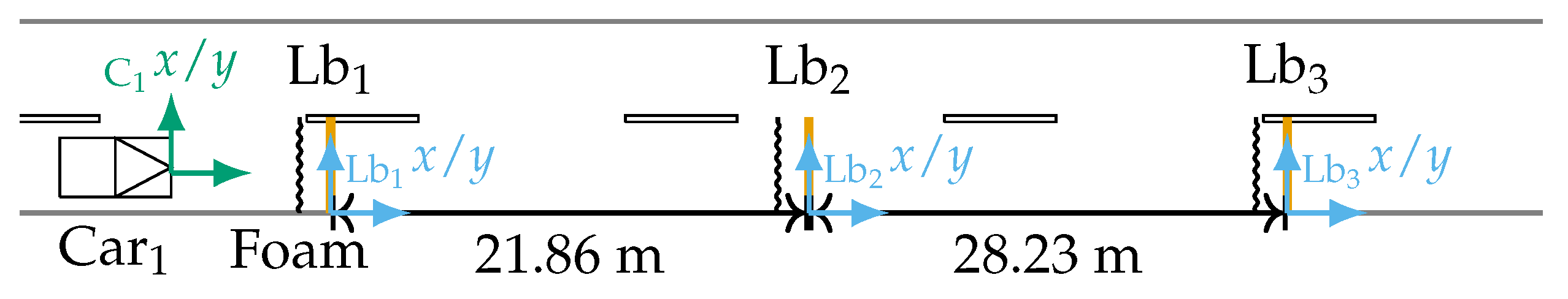
4.2.3. Absolute Positioning in Dynamic Case

To investigate the absolute accuracy of the reference measurement technique in the dynamic case, the following experiment is proposed: a vehicle passes through three light barriers designated as Lb₁, Lb₂, and Lb₃. These are aligned perpendicular to the roadway. The timesteps $t_{{\mathrm{Lb}}_{1...3}}$ at which a light barrier is crossed mark the point in time with zero longitudinal offset between the light barrier and the front point of the vehicle in a light barrier-centered coordinate system. In addition, a foam line is drawn perpendicular to the road. The measurement principle of the super-reference is again completely different to the ADMA and therefore this experiment is suitable as a super-reference. The full measurement setup is illustrated in Figure 5.

The error of the reference system is found at each light barrier as

$${ϵ}_{\mathrm{lat}}\left(t_{{\mathrm{Lb}}_{1...3}}\right)={}_{{\mathrm{C}}_1}{x}_{\mathrm{Ref}}\left(t_{{\mathrm{Lb}}_{1...3}}\right)-{}_{{\mathrm{Lb}}_{1...3}}{x}_{\mathrm{SRef}}\left(t_{{\mathrm{Lb}}_{1...3}}\right).$$

(3)

and when crossing the foam line, the lateral error can be determined based on the tire marks that remain on the foam. The lateral offset can only be determined at the wheels. The imprint of the tires is determined with a measurement tape and gives the lateral distance between the light barrier and the wheels. To account for the offset between the front of the vehicle and the front axle, the foam line is applied in front of the light barrier with an offset by this amount to minimize errors due to yaw angles. In other words, the longitudinal offset is known at the time at which the light barrier is crossed and should be zero. The longitudinal error is obtained at $t_{{\mathrm{Lb}}_{1...3}}$ for each light barrier and reads:

$${ϵ}_{\mathrm{long}}\left(t_{{\mathrm{Lb}}_{1...3}}\right)={}_{{\mathrm{C}}_1}{y}_{\mathrm{Ref}}\left(t_{{\mathrm{Lb}}_{1...3}}\right)-{}_{{\mathrm{Lb}}_{1...3}}{y}_{\mathrm{SRef}}\left(t_{{\mathrm{Lb}}_{1...3}}\right).$$

(4)

The experiment is conducted with the vehicle passing the light barriers at a constant velocity of 30 km/h and with an initial set speed of ${\dot{x}}_{{\mathrm{C}}_1}$ = 100 km/h at Lb₁ and braking. When the vehicle is decelerated while passing through the light barriers, the accuracy of the positioning in the dynamic case can be studied. Crossing the barriers with constant velocity indicates the potential sensitivity of positioning errors to velocity.

Three SICK WL 12-2 light barriers that have a specified delay time of 330 $\mathsf{\mu }$s are chosen for use in the experiment. The light barriers are connected to a second ADMA that is placed stationary next to Lb₂. Time synchronization between both devices is given by timestamps conveyed in the GNSS signal. Both ADMAs operate with $f_{\mathrm{s}}$ = 1000 Hz to minimize the positioning error due to sampling discretization.

The position of the light barriers in GNSS coordinates is measured with the RTK-aided Piksi Multi GNSS Module by Swift Navigation. The position of the point is averaged by measurement over 60 s. The verification of these GNSS coordinates is given as it matches the distance between the light barriers, which is determined by a measuring tape with mm accuracy. The spherical GNSS coordinates are converted into an East-North-Up (ENU) coordinate system based on the WGS84 ellipsoid, which is a metric Cartesian system.

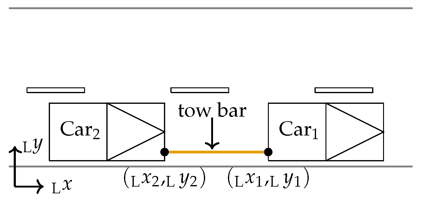
4.2.4. Relative Positioning between Vehicles in Dynamic Case

To determine the accuracy of the ADMA in the dual measurement setup under dynamic conditions, a constant distance between the two vehicles can be used. A tow bar mounted between two vehicles fulfills the requirement between the respective mounting points, also while driving. The position of the towing lugs on the vehicles relative to the ADMA is defined as a POI. By using the positioning information obtained, the calibration goal is to obtain the length of the tow bar, denoted $l_{\mathrm{tb},\mathrm{Ref}}$, which is assumed constant when neglecting strain effects of materials. Then, the resulting error, i.e., ${ϵ}_{\mathrm{tb}}=l_{\mathrm{tb},\mathrm{Ref}}-l_{\mathrm{tb},\mathrm{SRef}}$, is obtained, which should give zero for an ideal measurement. Measured length $l_{\mathrm{tb},\mathrm{SRef}}$ by a measuring tape of the tow bar is defined as the Euclidean distance of the measured mounting points in Cartesian world coordinates, i.e.,

$$l_{\mathrm{tb},\mathrm{Ref}}={∥\left(\begin{array}{c}{}_{\mathrm{L}}{x}_2{-}_{\mathrm{L}}{x}_1\\ {}_{\mathrm{L}}{y}_2{-}_{\mathrm{L}}{y}_1\end{array}\right)∥}_2$$

(5)

Car₁ accelerates from standstill to a given set speed. After a period of constant velocity, the front vehicle brakes the convoy to standstill. The velocity is controlled by Car₁’s speed limiter, while Car₂ rolls behind in towing mode, i.e., neutral gear position. Three velocity profiles were studied, each with multiple repetitions.

• 0 → 30 km/h → maintaining → 60 km/h → maintaining → 30 km/h → maintaining → 0
• 0 → 30 km/h → maintaining → 0
• 0 → 80 km/h → maintaining → 0

The profiles differ in the duration and intensity of acceleration or deceleration, as well as the duration of cruising at “constant” speed. In this way, the influence of these motion phases on the error can be studied. It is to be noted that the set speed of the speed limiter is the speedometer value, which is above the actual GT speed. The general scenario setup is shown in Figure 6.

5. Super-Referencing Results Obtained in Practical Experiments

The proposed super-reference methods were performed at the August Euler airfield near Darmstadt, Germany, between April and September 2021. The ADMA devices used were mounted, measured, and initialized according to the manufacturer’s instructions. A 2015 VW Golk Mk7 and a 2018 Mercedes S Class V222 were available as test vehicles.

5.1. Yaw Angle

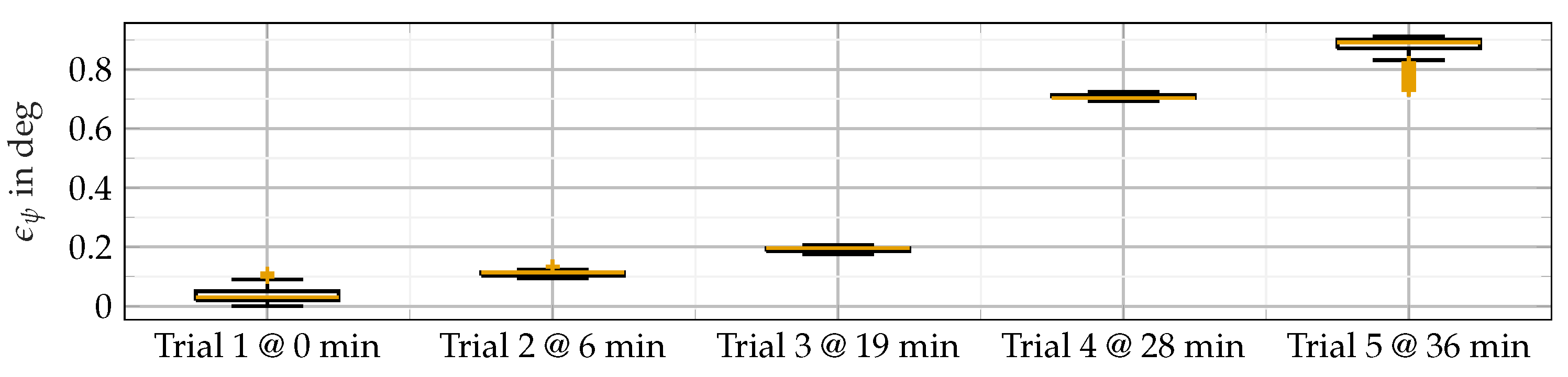
Figure 7 shows the results of our yaw angle referencing experiment. It compares the heading angle as calculated from the law of cosine to the measured value from the ADMA, i.e., ${ϵ}_{\psi }=|{\psi }_{\mathrm{Ref}}-{\psi }_{\mathrm{SRef}}|$. The experiment was conducted five times at various positions and data were collected for around 60 s each. The vehicles were moved only for the purpose of changing position and were otherwise stationary, especially during the determination of the super-reference, which took a couple of minutes. Stationary operating conditions particularly favor the occurrence of yaw angle drift. The drift objectively shows little effect and the deviations are less than 1 deg even after 36 min. It should be noted that the IMU and GNSS fusion system utilizes the dynamic movements of the device. Such a stationary experiment over a long time is challenging for the system. Drift is therefore an expected side effect.

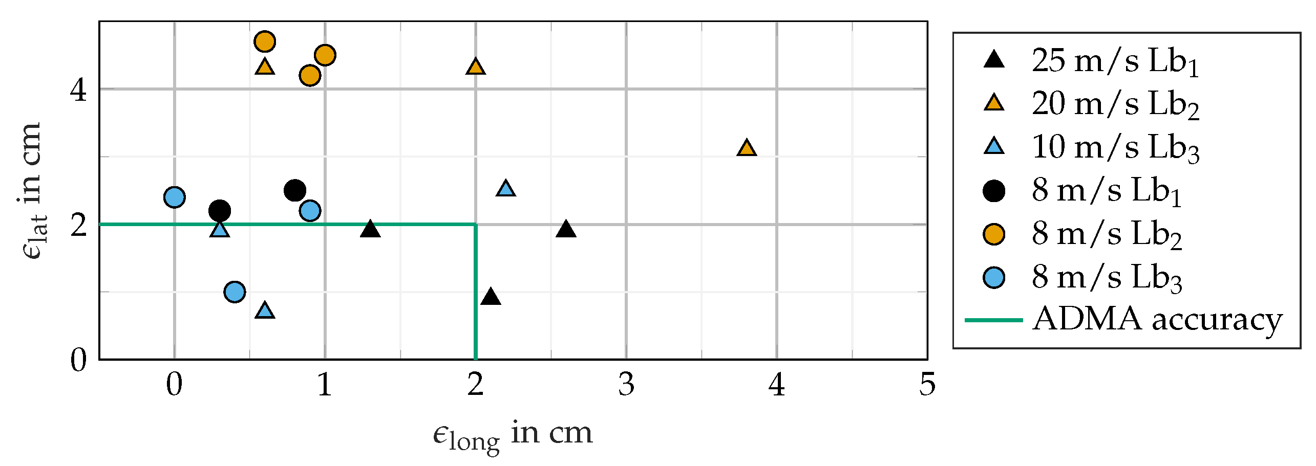
5.2. Absolute Positioning in Dynamic Case

The results of the super-referencing absolute positioning in the dynamic case by using light barriers (see Section 4.2.3) are shown in Figure 8. The lateral and longitudinal errors are denoted by ${ϵ}_{\mathrm{lat}}$ and ${ϵ}_{\mathrm{long}}$, respectively.

In general, high longitudinal and lateral precision in the three trials of every experiment and light barrier position is achieved. It is to be noted that ${ϵ}_{\mathrm{long}}$ is larger with a higher speed of the vehicle as it crosses the light barrier. Therefore, low velocities should be used as target velocities to achieve sufficient accuracy or devices with higher sampling frequencies. This is explained with measurement errors due to the light barrier’s time delay $\Delta t_{\mathrm{Lb}}$ = 330 $\mathsf{\mu }$s [22]. This explains the decreasing deviation in the longitudinal direction with decreasing speed, visible by the triangle markers. The delay results in a worst-case error at 25 m/s of

$${ϵ}_{\mathrm{long},\max }={\dot{x}}_{{\mathrm{C}}_1,\max }\Delta t_{\mathrm{Lb}}=8\mathrm{mm}@25\mathrm{m}/\mathrm{s}.$$

(6)

The remaining deviation is the error of the ADMA and the positioning error of the experimental setup. The lateral error ${ϵ}_{\mathrm{lat}}$ of our calibration method shows deviations higher than the proclaimed accuracy of the ADMA consistently present at the second light barrier. It shows deviations of around 2.5 cm from the proclaimed accuracy and indicates the experimental setup error. The ADMA’s error in the absolute dynamic case with a low velocity is always positive and differs between 0 cm and 3.8 cm in the longitudinal and 0.5 cm and 4.5 cm in the lateral direction.

5.3. Relative Positioning in Dynamic Case

The relative positioning error in the dynamic case is obtained by estimating the length of a tow bar mounted between two vehicles while driving; see Section 4.2.4. Figure 9 shows exemplary results obtained during one trial of the experiment. It is structured as follows: the error, which is obtained when estimating the tow bar length, i.e., ${ϵ}_{\mathrm{tb}}$, varies within ±3 cm. Because of the dual measurement setup, the worst-case error based on (5) and $\Delta x_{1/2}=\Delta y_{1/2}=\Delta x=\pm 2\mathrm{cm}$ is:

$$\Delta {ϵ}_{\mathrm{tb}}=\sqrt{{(\Delta x_1+\Delta x_2)}^2+{(\Delta y_1+\Delta y_2)}^2}=2\sqrt{2}\Delta x=5.7\mathrm{cm}$$

(7)

Therefore, the deviation of the devices is in accordance with their specification. Longitudinal acceleration in Car₁ or Car₂ with the fixed coordinate system shows little difference due to the mechanical coupling by the tow bar, which causes crabbing at the rear car. Moreover, the velocity profile is shown and does not indicate a strong correlation between error dynamics and longitudinal acceleration.

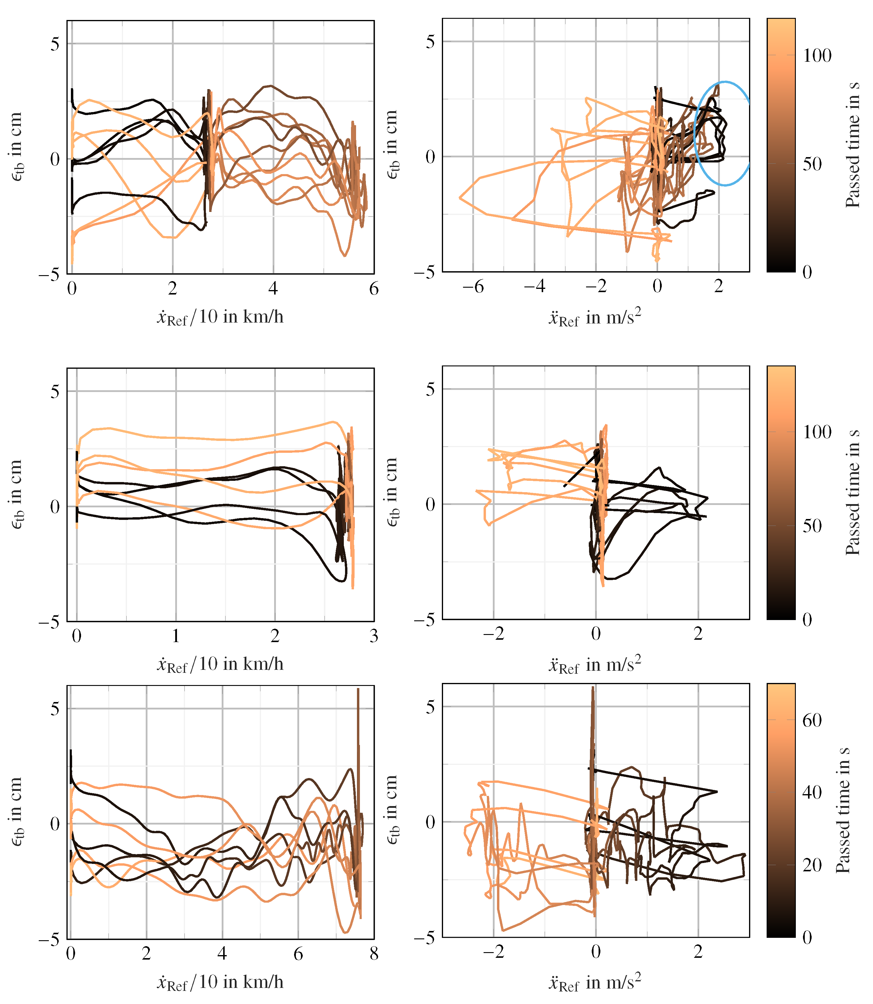
In Figure 10, the influence of velocity and acceleration on ${ϵ}_{\mathrm{tb}}$ is shown. The time course of the velocity or acceleration profile is coded in the color gradient from black to light brown and all trials of the experiment are shown. Studying the sensitivity of ${ϵ}_{\mathrm{tb}}$ to velocity reveals three consistent characteristics for all tests; see the left column in Figure 10.

• The error shows a fluctuation range of approximately 2 cm during quasi-stationary driving and matches the specification.
• During acceleration and braking phases, the error remains at a tolerable constant value within the fluctuation range.
• When reaching standstill, the error settles at a certain value, which lies inside the specification of the dual measurement setup.

No consistent correlations follow from the acceleration profile, as shown in the right column of Figure 10. However, it can be seen that the error also changes during the acceleration phases in the range of a few cm. It is worth noting, however, that the error profile shows some consistency when the acceleration profile is similar, as shown in the portion highlighted by a light blue ellipse in the right column and the first row of Figure 10.

6. Feasibility of Transferring Real-World Test Drives to Simulation

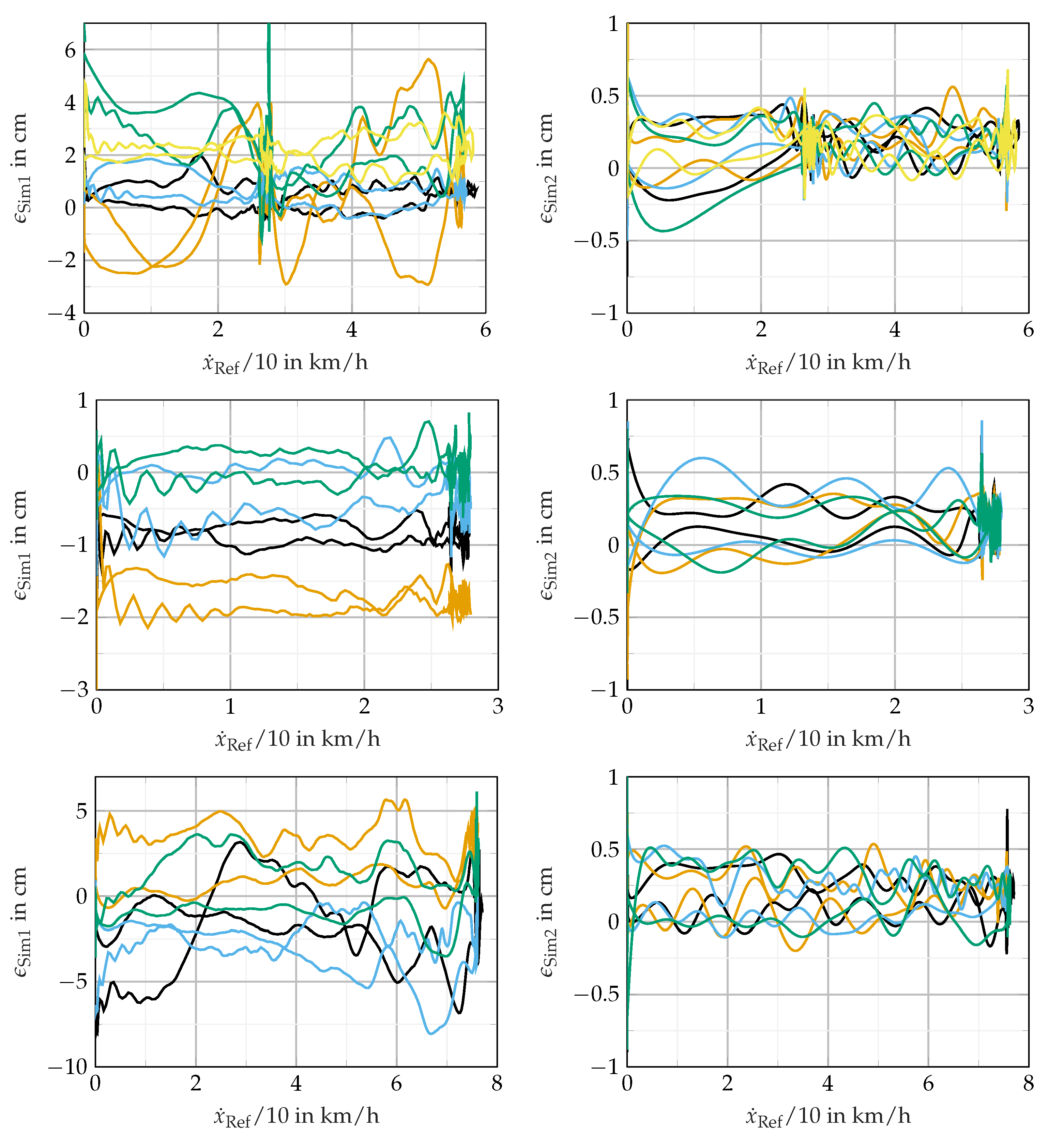
The main interest in using reference sensors in the context of virtual validation is ultimately to transfer real-world test drives to virtual environments. Under the so-called “Measurement2Sim” method, modern simulation tools such as IPG CarMaker, Vires VTD, or CARLA are able to control an actor’s position based on a given trajectory. The tow bar experiments are suitable to represent a simulation’s capability to render recorded measurements in the movement of objects. For this purpose, these experiments were transferred to two different simulation environments: Sim1 and Sim2.

The results are given in Figure 11 and are organized as follows. The left column shows the error ${ϵ}_{\mathrm{Sim}1}$ of the first simulation and the right column shows the error ${ϵ}_{\mathrm{Sim}2}$ of the second simulation. The topmost figures show five trials of the experiment, where the two vehicles undergo two phases of acceleration and deceleration with semi-stationary drive in between, i.e., from 0 to 30 km/h, 30 km/h to 60 km/h, back to 30 km/h, and finally to 0. The middle figures show the experiment with 30 km/h and the bottom figures with 80 km/h. The figures visualize the error between the reference measurement, as discussed in Section 5.3, and the simulation environment. Zero error would indicate that the measurement of the distance between vehicles, obtained either in simulation or via the reference measurement, exactly corresponds to the length of the tow bar.

$${ϵ}_{\mathrm{Sim}1/2}=(l_{\mathrm{tb},\mathrm{Sim}1/2}-l_{\mathrm{tb},\mathrm{Ref}})$$

(8)

The experiments show that the resulting deviations vary between trials through all trials of the experiments. The error in both simulation tools thereby shows sensitivity to velocity: from the results shown, it can be concluded that the error becomes less with lower speeds, while showing the largest error during phases of acceleration or deceleration. In the first simulation during phases of semi-stationary velocities, the error occasionally extends the proclaimed accuracy of the ADMA. In the second simulation, in turn, the errors are always in the accuracy range.

Our results show that the reenacting of test drives performs best with the first simulation tool when the velocities of the vehicles are kept fairly constant and the accelerations are low, i.e., less than 2 m/s${}^2$. The absolute deviation between measurement and simulation is in orders of magnitude exceeding the distance resolution of lidar sensors or high-resolution radar sensors. This makes the comparison of simulation to measurement considerably more difficult, since the basis of comparison shows deviations.

7. Discussion

In this paper, we present four different experimental setups to obtain super-reference measurements. With the proposed methods, the confidence in GNSS- and IMU-based reference data for lateral and longitudinal positions can be strengthened in stationary and dynamic cases, as well as the drift analysis of the stationary yaw angle. We note that the highest precision is required when setting up the measurement equipment in order to achieve useful results in terms of super-referencing. During our experimental setups, we encountered the necessity of excellent measuring conditions regarding GNSS measurement devices, because the accuracy of the device’s data is highly dependent on the surrounding conditions. Effects such as multipath propagation, shading by other objects, and loss of differential GNSS and RTK connection result in deviation that is an order of magnitude above ideal conditions.

Our experiments reveal the strengths and weaknesses of the reference system under study, the ADMA. The stated measurement accuracy is almost consistently met. The yaw angle measurement quantifies the expected drift of the device. The reference system confirms the proclaimed accuracy during the light barrier experiment. The experiment shows the difficulty in verifying the position accuracy by means of the super-reference, showing less deviation than the system under test. In the dynamic dual measurement setup with the tow bar, the deviation always lies within the specification.

Our comparison of the simulation and real test drive shows a new possibility of verifying the fidelity of so-called “Measurement2Sim” methods. Not only the transfer of the trajectory into the simulation is a source of deviations between measurements and simulation, but also the simulation tool itself provides errors due to the trajectory discretization. The results between the two simulation tools differ clearly. The sources of the deviations cannot be directly identified. When the “Measurement2Sim” method is used in the context of validation of sensor models, it has to be noted that the deviation must not exceed the accuracy of the sensor itself. In the case of lidar, typically, accuracy lies within in the centimeter range. The second simulation tool is better suited to reproducing sensor effects in sensor simulation models with the “Measurement2Sim” method. This simulation tool converts the trajectories very well on the basis of an OpenScenario xosc file based on the measurements of $\mathbf{x}=[x,y,z,\varphi ,\theta ,\psi ]$. For future verification and validation experiments in combination with “Measurement2Sim” methods, we highly recommend the analysis of the transfer error of the measurement into the simulation.

Regarding virtual validation by means of digital twins, our results indicate that sample validation using “reference measurement sensors” can hardly be achieved. This is of particular importance when considering the accuracy of perception sensors, which is close to the stochastic deviation margin of the reference measurement system. Rather, our findings strengthen the argumentation for stochastic validation approaches that explicitly take the measurement uncertainties of the reference system into account.