A Computer Tool Using OpenModelica for Modelling CO₂ Emissions in Driving Tests

Abstract

The transport sector is one of the main barriers to achieving the European Union’s climate protection objectives. Therefore, more and more restrictive legal regulations are being introduced, setting out permissible limits for the emission of toxic substances emitted into the atmosphere, promoted biofuels and electromobility. The manuscript presents a computer tool to model the total energy consumption and carbon dioxide emissions of vehicles with an internal combustion engine of a 2018 Toyota Camry LE. The calculation tool is designed in the OpenModelica environment. Libraries were used for this purpose to build models of vehicles in motion: VehicleInterfaces, EMOTH (E-Mobility Library of OTH Regensburg). The tool developed on the basis of actual driving test data for the selected vehicle provides quantitative models for the instantaneous value of the fuel stream, the model of the instantaneous value of the carbon dioxide emission stream as a function of speed and the torque generated by the engine. In the manuscript, the tests were conducted for selected driving cycles tests: UDDS (EPA Urban Dynamometer Driving Schedule), HWFET (Highway Fuel Economy Driving Schedule), EPA US06 (Environmental Protection Agency; Supplemental Federal Test Procedure (SFTP)), LA-92 (Los Angeles 1992 driving schedule), NEDC (New European Driving Cycle), and WLTP (Worldwide Harmonized Light-Duty Vehicle Test Procedure). Using the developed computer tool, the impact on CO₂ emissions was analyzed in the context of driving tests with four types of fuels: petrol 95, ethanol, methanol, DME (dimethyl ether), CNG (compressed natural gas), and LPG (liquefied petroleum gas).

1. Introduction

The carbon-intensive road transport sector faces enormous technological, social, entrepreneurial, and managerial challenges [1,2,3]. Awareness of environmental threats and social pressure are the prerequisites for introducing more and more restrictive regulations on the amount of pollutant emissions [4,5,6].

Member States and the European Union (EU) have been following a path of emission reductions since at least 1997, the Kyoto Protocol, the Doha Amendment of 2012, the Paris Agreement of 2015, and the European Green Deal of 2019, which set out a path for the development of Member State economies in view of an ambitious EU-wide climate target of climate neutrality by 2050, and the vast majority of which is addressed to road transport [7,8,9,10].

In the Paris Climate Agreement, the EU undertook to reduce greenhouse gas emissions by at least 40% by 2030 in all economic sectors compared to the 1990 levels. However, in the 2020 strategy, complementary to the “European Green Deal”, “Sustainable and Smart Mobility Strategy—putting European transport on track for the future”, the main goal in the field of mobility is a 90% reduction in emissions from all transport by 2050 [11,12].

According to the latter document, the entire internal combustion vehicle market is to be subject to stricter emission standards, and the regulations concerning CO₂ emission standards for cars and vans are to be revised. In addition, the road charging system is to be tightened up and made more efficient. A significant change is the possible inclusion of road transport in the European CO₂ emissions trading scheme. The above changes are to motivate road users to increase the number of ecological vehicles, i.e., to promote the development of solutions that are energy-efficient and possibly the least harmful to the environment. European Union authorities want 30 million electric cars on the roads of EU member states by 2030. There are 313 million cars registered in the EU. This means that in 2030, almost every tenth vehicle would be electric. Currently, 1.4 million such vehicles are registered for electricity in the member states. According to a report by the European Automobile Manufacturers’ Association (ACEA), in the third quarter of 2020, the number of petrol cars registered in EU countries fell by 24.3%, diesels by 13.7%, and electric cars increased by 132 % compared to the comparable period in 2019. Demand for diesels and petrol vehicles is decreasing, although petrol cars still account for more than half of the EU market [13,14,15].

When analyzing the environmental performance of vehicles, it is important to look at how they interact with the environment from production, through the time of use, to disposal. It should be noted that the value of eco depends very much on the driver, and their driving habits and technique. Electric cars are locally zero-emission. Where they are used, they emit no fumes and do not pollute the surrounding air. The extent to which an electric car is truly zero-emission is determined by the source of energy used to power the battery. If we are dealing with so-called green energy—coming from renewable sources (e.g., a wind turbine or our own photovoltaic installation), the carbon footprint of an electric vehicle is limited only to the production stage. If this energy comes mainly from coal-fired power plants, you still have to take into account the CO₂ emissions from power generation.

CO₂ emissions from passenger transport vary considerably depending on the mode of transport. Passenger cars are the main source of pollution, accounting for 60.7% of all CO₂ emissions from road transport in Europe. It should also be stressed that the dynamics of historical CO₂ emissions from the transport sector in individual EU member states are different. For example, in Poland, between 2005 and 2017, a significant increase in emissions was observed (by 76%), where in the EU, a decrease in emissions of 3% was visible during the same period. In order to analyze the possibilities of reducing emissions in the transport sector, scenarios are created that include carbon-dependent charges included in the purchase price of fuels against the background of ongoing technological progress [16,17,18,19].

In order to reduce the emission of car exhausts, legal regulations are created, defining upper limits for the content of particular toxic components in exhaust gases [20,21].

In the area of the European Union, periodical vehicle technical inspections have been obligatory since 1992 [22,23]. Their purpose is to assess the technical condition of the vehicle, on the basis of which it may be admitted to road traffic. Apart from the limit values for the mentioned components of the vehicle exhaust gases, the standards also define the methodology of emission tests in specially adjusted laboratories. During inspection, the functioning of the elements aimed at reducing the harmful impact on the environment is checked, among others. The standards regulate the emission of nitrogen oxides, carbon oxides, hydrocarbons, and particulate matter in cars that drive on the road. Cars currently sold should meet the EURO 6 standard from 2014 [24,25,26]. Exhaust emission standards in force in Europe define different requirements for the engines of passenger cars and vans, as well as trucks and buses. Protection of air cleanliness is a priority of the European Commission, therefore, from time to time, the standards are changed and the limit values given in them are reduced, so as to mobilize the car companies to look for new, better technological solutions that will be a lower burden on the environment [27,28,29,30]. At the moment, the tightening of regulations concerning the reduction of the emission of toxic compounds in engine exhaust gases, fuel consumption, and the emission of greenhouse gases is the main factor steering the direction of development of motor vehicle designs.

Throughout the European Union, a new type of vehicle is allowed for sale after obtaining an approval certificate. Such a document is issued by the appropriate national authority and proves that the prototype meets all EU requirements concerning safety, environmental protection, and conformity of production [31,32]. Emissions are tested both in laboratory conditions (WLTP (World Harmonized Light Vehicle Test Procedure)) and on the road (RDE (Real Driving Emissions)). Laboratory tests, which are conducted according to a standardized and repeatable procedure, enable consumers to compare different car models [33,34,35,36].

WLTP is a new global harmonized test procedure for light commercial vehicles developed to measure fuel consumption, CO₂, and pollutant emissions for passenger cars and light commercial vehicles. The maximum speed during testing is 131.3 km/h. The average speed is 46.5 km/h and the total cycle time is 30 min. The distance covered during the test is 23.25 km [37,38]. The WLTP test consists of four parts, depending on the maximum speed: low (the test lasts 589 s, the car covers 3 km, accelerates to the maximum 56.5 km/h and reaches an average speed of 18.9 km/h), medium (the test lasts 433 s, the car covers 4.7 km, accelerates to 76.6 km/h and reaches an average speed of 39.4 km/h), high (the test lasts 455 s, the car covers 7.2 km, accelerates to 97.4 km/h and reaches an average speed of 56.5 km/h), and very high (the test lasts 323 s, the car covers 8.3 km, accelerates to 131.3 km/h and reaches an average speed of 94 km/h). Individual parts of the cycle simulate urban driving, suburban driving on roads other than urban and motorways. The cycle also does not simulate hill climbs. The procedure also takes into account all optional vehicle accessories affecting aerodynamics, such as rolling resistance or vehicle mass, which have an impact on vehicle-specific CO₂ emissions [39,40]. WLTP includes guidelines for new driving cycles ((WLTC) Worldwide harmonized Light-duty vehicles Test Cycles).

The RDE test is not a substitute for laboratory testing, but complements it, especially for NOx emissions. Real-world emission testing involves measuring pollutants using portable emissions measurement systems (PEMS) mounted on cars as they drive on the road. The vehicle is driven on a real road according to randomly selected parameters such as acceleration, deceleration, ambient temperature, and load [41,42]. The limits that cannot be exceeded are defined as those obtained from the laboratory test (WLTP), multiplied by the influencing factors. The compliance factors take into account the margin of error of the instrumentation, which is not the same as the level of accuracy and repeatability in the laboratory test.

Until 2017, the New European Driving Cycle (NEDC) test procedure was in force within the European Union. The NEDC included two test phases: the UDC (urban driving cycle) and the EUDC (extra urban driving cycle). For 13 min, the vehicle is tested in what is assumed to be urban conditions, with the remaining 7 min in non-urban conditions. The components of this cycle do not take into account actual driving patterns and distances travelled on different types of roads. The average speed over the NEDC cycle is only 34 km/h and the maximum speed is only 120 km/h. The total distance the vehicle covers in the test is 11 km [43,44].

In the United States of America, the FTP-75 (Federal Transient Procedure) test is used to assess the environmental performance of passenger cars and light-duty vehicles, and the Highway Federal Extra Test (HWFET) is used to assess fuel consumption [45,46].

The federal test procedure (FTP) consists of the UDDS (Urban Dynamometer Driving Schedule). The Urban Dynamometer Driving Schedule is a mandatory test on a dynamometer of a car’s tailpipe emissions. The cycle consists of two phases. In the first phase, the vehicle covers a distance of 5.78 km at an average speed of 41.2 km/h in 505 s. In the second phase, which takes 864 s, the vehicle covers a distance of 6.29 km. The maximum speed reached by the vehicle during the test is 91.2 km/h [47,48].

The FTP-75 cycle consists of four phases. During the whole cycle, the car covers a distance of 17.77 km, in 1877 s, at an average speed of 34.12 km/h (maximum speed of 91.25 km/h). Additionally, cars must be tested under two supplemental federal test procedures ((SFTP) Supplemental Federal Test Procedures): aggressive driving (SFTP US06) and the optional air conditioning test (SFTP SC03) [49,50,51,52].

The Highway Fuel Economy Test (HWFET) is used to determine the highway fuel economy rating. During the cycle, which takes 765 s, the car covers a distance of 16.45 km, with an average speed of 77.7 km/h [53,54].

In addition, there is the standardized LA92 cycle, which, compared to FTP, has a higher maximum and average speed, shorter idle time, fewer stops, and a higher maximum acceleration rate. LA-92 is designed for Class 3 heavy-duty vehicles [55,56].

One of the most popular fuels in the world is petrol. Raw petrol has a low resistance to pre-ignition, so it is enriched with special compounds that decrease the “knocking” effect. In a controlled way, fuel with different octane numbers can be obtained, which is tailored to the needs of specific engines and does not cause damage to them [57,58].

LPG (liquefied petroleum gas) is an alternative power source for internal combustion engines. This fuel is a mixture of liquefied propane and butane. Due to climatic differences, the proportions of the components can vary [59,60].

Compressed natural gas (CNG) is a gas compressed to 20–25 MPa, consisting of approximately 97% methane. CNG is distinguished by its high octane number (130) and has the highest efficiency among liquid fuels [61,62].

For many years, intensive research has been carried out in the direction of alternative fuels. Considering the engine being powered by different fuels, the same energy conversion efficiency must be assumed. With this assumption, it is possible to calculate the mass of a given fuel, the combustion of which yields energy equal to the energy obtained from burning 1 kg of gasoline, and then to calculate the carbon dioxide emissions, also with respect to the emissions produced by burning 1 kg of gasoline.

The question of biofuels’ influence on the reduction of CO₂ emission is complicated and requires taking into consideration, apart from the chemical composition, many factors connected with the type of construction and the specificity of the engine operation. It has been claimed in the literature that methane is the only commonly used engine fuel that results in a significant reduction of carbon dioxide emissions compared to gasoline engine fueling [63].

A separate issue is the use of plant-based fuels to power engines. These are mainly alcohols used to power spark ignition engines and various types of vegetable oils or their esters used to power compression ignition engines. Using them in pure form (alcohols) or mixed with gasoline (E85 fuel) results in higher carbon dioxide emissions than using gasoline. A similar effect occurs when compression ignition engines are fueled with vegetable oils.

For example, methyl and ethyl alcohols are used as engine fuels. They are used in pure form or as additives and as a raw material to produce MTBE (methyl tert-butyl ether) and ETBE (ethyl tert-butyl ether). The biggest disadvantage of ethanol is its low calorific value. In relation to a liter, this value is 1/2 lower than in the case of petrol (petrol in accordance with PN-EN228 42.3–43.5 MJ/kg; ethanol 26.8 MJ/kg). The cetane number of ethanol is 8. The properties of methanol are similar to ethanol, but it has an even lower calorific value (20.1 MJ/kg) and is a strong poison [64,65,66,67].

An alternative fuel for powering motor vehicles that is the subject of much research is dimethyl ether (DME) [68,69]. This fuel can be produced from many sources such as natural gas, coal, and biomass. DME is characterized by a very high cetane number. The physicochemical properties of DME are similar to LPG.

Dedicated tools for performing computer simulation analysis of the amount of pollutants emitted from motor vehicles have been in the works for many years.

An example of such a tool is VECTO (Vehicle Energy Consumption Calculation Tool) [70,71]. A simulation tool is used to calculate the amount of fuel consumed and the carbon dioxide emitted by new trucks.

The tool to run a simulation showing what results a given vehicle with WLTP testing would achieve in the NEDC test was CO2MPAS (CO₂ Model for Passenger and commercial vehicles Simulation) [72,73].

A literature review finds tools for analyzing bus fleet emissions in an urban area [74].

There is a lack of tools, developed in an open source environment, that can be adapted to the operational parameters of a large set of vehicles that represent a given car market.

The aim of the study was to build a computer tool for modelling selected driving tests, fuel and biofuel consumption, and CO₂ emissivity analysis. The developed tool, using tests on a chassis dynamometer and unit fuel consumption and the resistance of working elements, is dedicated to vehicles with spark-ignition engines. In order to achieve the aim of the study, the OpenModelica environment was used.

2. Materials and Methods

2.1. Basic Information

The list below contains a set of the most important quantities used in the calculations with the appropriate symbols and units (

Table 1. Abbreviations, symbols and units used in the paper.

Parameter	Description	Unit
${\mathrm{T}}_{\mathrm{reg}}$	Instantaneous torque value calculated in the engine master PID controller	N⋅m
${\mathrm{T}}_{\mathrm{engloss}}\left({\mathsf{\omega }}_{\mathrm{eng}}\right)$	Instantaneous torque function of the mechanical losses of the test engine	N⋅m
${\mathrm{I}}_{\mathrm{eng}}$	Engine moment of inertia for rotary motion	kg·m2
${\mathsf{\omega }}_{\mathrm{eng}}$	Engine instantaneous crankshaft angular velocity	rad/s
${\mathrm{v}}_{\mathrm{veh}}$	Instantaneous vehicle velocity for road test	m/s
${\mathrm{v}}_{\mathrm{set}}$	Instantaneous set vehicle velocity in road test	m/s
${\mathrm{T}}_{\mathrm{engmax}}\left({\mathsf{\omega }}_{\mathrm{eng}}\right)$	Instantaneous value of the maximum torque at the engine crankshaft as a function of the engine angular velocity	N⋅m
$\mathrm{PID}\left({\mathrm{v}}_{\mathrm{set}}-{\mathrm{v}}_{\mathrm{veh}}\right)$	PID controller function value	N⋅m
${\mathsf{\omega }}_{\mathrm{eng}}$	Instantaneous angular velocity of the engine crankshaft	rad/s
${\mathsf{\omega }}_{\mathrm{tcin}}$	Instantaneous angular velocity at the torque amplifier input	rad/s
${\mathsf{\omega }}_{\mathrm{tcout}}$	Instantaneous angular velocity at the torque amplifier output	rad/s
$\mathrm{K}\left(v\right)$	K-factor function (torque amplifier input velocity divided by torque amplifier input root)	rpm/(N⋅m)½
$\mathsf{{\rm M}}\left(v\right)$	Torque amplifier conversion factor function	-
${\mathrm{T}}_{\mathrm{tcout}}$	Instantaneous torque value calculated by the torque amplifier	N⋅m
${\mathrm{T}}_{\mathrm{gbloss}}\left({\mathsf{\omega }}_{\mathrm{tcout}},{\mathrm{r}}_{\mathrm{gb}}\right)$	Instantaneous torque value of mechanical losses in transmission	N⋅m
${\mathrm{r}}_{\mathrm{gb}}$	Instantaneous gearbox ratio value	-
${\mathrm{R}}_{\mathrm{div}}$	Value of differential ratio	-
${\mathrm{T}}_{\mathrm{brakemax}}$	Maximum braking torque value for the vehicle	N⋅m
$\mathrm{A}$	Load coefficient	N
$\mathrm{B}$	Load coefficient	N/(km/h)
$\mathrm{C}$	Load coefficient	N/(km/h)2
${\mathrm{T}}_{\mathrm{dtout}}$	Instantaneous value of the torque produced by the drive train	N⋅m
${\mathrm{T}}_{\mathrm{brake}}$	Instantaneous brake torque value	N⋅m
${\mathrm{M}}_{\mathrm{fuelEPA}}\left({\mathrm{T}}_{\mathrm{eng}},{\mathsf{\omega }}_{\mathrm{eng}}\right)$	Fuel flow value function (based on published EPA data)	kg/s
${\mathrm{T}}_{\mathrm{eng}}$	Torque produced at engine crankshaft	N⋅m
${\mathrm{Cal}}_{\mathrm{fuel}}$	Calorific value of fuel used in actual EPA tests	J/kg
${\mathrm{Cal}}_{\mathrm{i} \mathrm{fuel}}$	Calorific value of another fuel	J/kg
${\mathrm{C}}_{\mathrm{i}}$	Mass fraction of carbon i in this fuel	kg/kg
${ṁ}_{{\mathrm{i} \mathrm{fuel}}_{\mathrm{i}}}$	Mass flow i of this fuel in the mixture	kg/s

).

The development of the simulation model for driving tests was based on the testing of the Toyota Camry LE vehicle and is published in [75].

The most important technical parameters of the vehicle and the necessary coefficients to be used in the driving tests are presented below in

Table 2. Parameters of the vehicle used in the research for driving tests [60,76].

Parameter	Description	Unit
Vehicle (MY, make, model)	2018 Toyota Camry LE	-
Equivalent test mass	1644	kg
Rated power (declared)	151@ 6600 min−1	kW
Rated Torque	249 Nm @ 4800 min−1	N⋅m
Emission Certification	Federal Tier 3 Bin 30/California LEV-III SULEV30	-
Fuel consumption (city/highway/combined)	62.5/44.9/54.7	g/km
CO₂ emissions (city/highway/combined)	190.1/136.5/166.4	g/km
Rated engine speed (declared)	7000	min−1
Idling engine speed (declared)	800	min−1
Max vehicle speed(declared)	240	km/h
Number of gears	8	-
Ratio gear 1	5.250	-
Ratio gear 2	3.028	-
Ratio gear 3	1.950	-
Ratio gear 4	1.456	-
Ratio gear 5	1.220	-
Ratio gear 6	1.000	-
Ratio gear 7	0.808	-
Ratio gear 8	0.673	-
Differential ratio [-]	2.802	-
Target Coeff f0	113.82	N
Target Coeff f1	0.5442	N/(km/h)
Target Coeff f2	0.02811	N/(km/h) 2

.

The simulation process used test results for actual tests conducted by the EPA on a selected vehicle:

• UDDS—The EPA Urban Dynamometer Driving Schedule [77,78];
• HWFET—The Highway Fuel Economy Driving Schedule [77,79];
• US 06—The high acceleration aggressive driving schedule, which is often identified as the “Supplemental FTP” driving schedule [77,80];
• LA92—The LA-92 is for Class 3 Heavy-Duty vehicles, the first 1435 s are the Hot LA-92 driving schedule [77,81];
• NEDC—New European Driving Cycle (NEDC) [82,83];
• WLTC 3b random—WLTP for Class 3 vehicles with an engine power above 34 W/kg [83,84,85,86].

2.2. Building a Quantitative Model

The simulation of the running tests, whose general scheme is shown in Figure 1, was developed in the OpenModelica numerical environment using the following libraries: “Modelica Standard”, “Modelica, Mechanics, Rotational”, and “Modelica, Mechanics, Translational”. The simulation consisted of modules that performed calculations corresponding to real assemblies in the vehicle. The module “test drive generator” during the start of the simulation reads from the mass memory prepared files containing the data of the driving test. Then, the signals—instantaneous set vehicle speed v_set and instantaneous value of gear ratio r_gb—are transferred to other modules. The “engine” module is responsible for the functionality of the internal combustion engine with the PID controller system. The PID controller (proportional-integral-derivative) calculates the value of the torque at the engine crankshaft T_eng on the basis of the set value of the vehicle speed and the vehicle speed resulting from the simulation run. Then, the drive is transferred to the “torque converter” module, where the output torque value T_tcout is amplified and the output speed ω_tcout on the torque amplifier shaft is decreased in relation to the input values. In the “drivetrain” module, the values of torque t_dtout and speed ω_dtout on the output shaft are calculated using the instantaneous values of gear ratio r_gb. The “vehicle” module, using the supplied drive from the “drivetrain” module, calculates the instantaneous value of the vehicle speed v_veh. In this module, a PID controller is used, which makes it possible, on the basis of the signal of the set speed of the vehicle v_set and the actual speed of the vehicle resulting from the simulation work, to perform the braking process. The module “fuel consumption, CO₂ emissions” is responsible for calculating the value of fuel consumption and CO₂ emissivity during the simulation.

In the “engine” module, the instantaneous value of the torque produced by the engine at crankshaft T_eng is calculated from the relationship shown below:

$${\mathrm{T}}_{\mathrm{eng}}={\mathrm{T}}_{\mathrm{reg}}-{\mathrm{T}}_{\mathrm{engloss}}\left({\mathsf{\omega }}_{\mathrm{eng}}\right)-{\mathrm{I}}_{\mathrm{eng}}\cdot \frac{{\mathrm{d}\mathsf{\omega }}_{\mathrm{eng}}}{\mathrm{dt}}$$

(1)

Figure 2a shows a diagram of torque losses T_engloss(ω_eng) as a function of the angular velocity of the engine crankshaft, which were used to calculate the torque generated by the engine on the crankshaft [75].

A PID controller algorithm was used to calculate the instantaneous torque T_eng of the engine in the simulation. Based on the difference between the set instantaneous vehicle speed in the test v_set and the actual instantaneous vehicle speed v_veh during the simulation run, it calculates the necessary torque value T_reg to obtain the minimum control error. In order to make the simulation as consistent as possible with real conditions, the maximum torque values of the controller were limited according to the characteristics of the maximum torque as a function of the angular velocity of the crankshaft of the engine under consideration ${\mathrm{T}}_{\mathrm{engmax}}\left({\mathsf{\omega }}_{\mathrm{eng}}\right)$. The graph showing the variation of the instantaneous values of the maximum torque at the engine crankshaft as a function of the crankshaft angular velocity is shown in Figure 2b [75].

The relationship below shows how the torque produced by the PID controller is calculated in the simulation:

$${\mathrm{T}}_{\mathrm{reg}}=\{\begin{array}{l}{\mathrm{T}}_{\mathrm{engmax}}\left({\mathsf{\omega }}_{\mathrm{eng}}\right),\mathrm{PID}\left({\mathrm{v}}_{\mathrm{set}}-{\mathrm{v}}_{\mathrm{veh}}\right)>{\mathrm{T}}_{\mathrm{engmax}}\left({\mathsf{\omega }}_{\mathrm{eng}}\right)\\ \mathrm{PID}\left({\mathrm{v}}_{\mathrm{set}}-{\mathrm{v}}_{\mathrm{veh}}\right),0\le \mathrm{PID}\left({\mathrm{v}}_{\mathrm{set}}-{\mathrm{v}}_{\mathrm{veh}}\right)\le {\mathrm{T}}_{\mathrm{engmax}}\left({\mathsf{\omega }}_{\mathrm{eng}}\right) \\ 0 \mathrm{N}\cdot \mathrm{m},\mathrm{PID}\left({\mathrm{v}}_{\mathrm{set}}-{\mathrm{v}}_{\mathrm{veh}}\right)<0\end{array}\}\left[\mathrm{N}\cdot \mathrm{m}\right]$$

(2)

Figure 3 shows the block diagram of the developed simulation responsible for calculating the instantaneous value of the torque produced at the engine crankshaft.

In the “torque converter” module, the torque produced by the engine is amplified. Based on the signals ${\mathsf{\omega }}_{\mathrm{tcout}}$ and ${\mathsf{\omega }}_{\mathrm{tcin}}$, the “speed ratio” $v$ is calculated. Then, the value of the torque at the input of the torque amplifier ${\mathrm{T}}_{\mathrm{tcin}}$ and the value of the torque produced at the output shaft of the torque amplifier ${\mathrm{T}}_{\mathrm{tcout}}$ are calculated. If the “speed ratio” $v$ reaches a value above 0.9, the torque amplifier is blocked and the input torque is equal to the output torque. In the simulation, elements implementing the calculations according to the relationships below are used, as follows:

$$v=\frac{{\mathsf{\omega }}_{\mathrm{tcout}}}{{\mathsf{\omega }}_{\mathrm{tcin}}}. \mathsf{\mu }=\mathsf{{\rm M}}\left(v\right),{ \mathrm{T}}_{\mathrm{tcin}}={\left(\frac{30\cdot {\mathsf{\omega }}_{\mathrm{tcin}}}{\mathsf{\pi }\cdot \mathrm{K}\left(v\right)}\right)}^2\left[\mathrm{N}\cdot \mathrm{m}\right]$$

(3)

$${\mathrm{T}}_{\mathrm{tcout}}=\{\begin{array}{l}\mathsf{\mu }\cdot {\mathrm{T}}_{\mathrm{tcin}},v<0.9\\ {\mathrm{T}}_{\mathrm{tcin}},v\ge 0.9\end{array}\}\left[\mathrm{N}\cdot \mathrm{m}\right]$$

(4)

In order to develop the torque amplifier simulation module, it was necessary to introduce the basic data of the real assembly into the environment. The graphs below (Figure 4a,b) show the waveforms used in the developed simulation of the values of the K-factor and the conversion ratio μ as a function of the speed ratio ν.

Figure 5 shows a diagram of the torque amplifier function simulation module and the calculation of the output torque value T_tcout passed on to further parts of the simulation.

The “drivetrain” module contains simulations of the functionality of the gearbox and the differential in the tested vehicle. In this case, based on the torque delivered from the torque amplifier ${\mathrm{T}}_{\mathrm{tcout}}$, the instantaneous values of the gearbox ratio ${\mathrm{r}}_{\mathrm{gb}}$, and the constant value of the differential ratio ${\mathrm{R}}_{\mathrm{div}}$, the calculation of the torque T_dtout transmitted to the wheels of the vehicle is carried out. The relationships enabling these calculations are presented below.

$${\mathrm{T}}_{\mathrm{dtout}}=\left({\mathrm{T}}_{\mathrm{tcout}}-{\mathrm{T}}_{\mathrm{gbloss}}\left({\mathrm{T}}_{\mathrm{tcout}}.{\mathrm{r}}_{\mathrm{gb}}\right)\right)\cdot {\mathrm{r}}_{\mathrm{gb}}\cdot {\mathrm{R}}_{\mathrm{div}}\left[\mathrm{N}\cdot \mathrm{m}\right]$$

(5)

$${\mathsf{\omega }}_{\mathrm{dtout}}=\frac{{\mathsf{\omega }}_{\mathrm{tcout}}}{{\mathrm{r}}_{\mathrm{gb}}\cdot {\mathrm{r}}_{\mathrm{div}}}\left[\frac{\mathrm{rad}}{\mathrm{s}}\right]$$

(6)

In this module, the calculation of the output torque ${\mathrm{T}}_{\mathrm{dtout}}$ takes into account the losses occurring in the transmission system. These losses in the form of the waveform of transmission torque variations as a function of shaft torque input and the value of the ratio ${\mathrm{T}}_{\mathrm{gbloss}}\left({\mathrm{T}}_{\mathrm{tcout}},{\mathrm{r}}_{\mathrm{gb}}\right)$ are shown in Figure 6.

Figure 7 shows the module responsible for the functionality of the gearbox and the differential.

In the “vehicle” module, the PID controller algorithm was used to calculate the instantaneous values of the braking force in the vehicle. Based on the calculated difference between the instantaneous vehicle speed ${\mathrm{v}}_{\mathrm{veh}}$ and the test set speed ${\mathrm{v}}_{\mathrm{set}}$ (the order has been changed because the PID controller calculates the braking force only if the vehicle speed is higher than the preset speed), the value of the vehicle braking torque ${\mathrm{T}}_{\mathrm{brake}}$ is calculated according to the relation below:

$${\mathrm{T}}_{\mathrm{brake}}=\{\begin{array}{l}{\mathrm{T}}_{\mathrm{brakemax}},\mathrm{PID}\left({\mathrm{v}}_{\mathrm{veh}}-{\mathrm{v}}_{\mathrm{set}}\right)>{\mathrm{T}}_{\mathrm{brakemax}}\\ \mathrm{PID}\left({\mathrm{v}}_{\mathrm{veh}}-{\mathrm{v}}_{\mathrm{set}}\right),0\le \mathrm{PID}\left({\mathrm{v}}_{\mathrm{veh}}-{\mathrm{v}}_{\mathrm{set}}\right)\le {\mathrm{T}}_{\mathrm{brakemax}} \\ 0 \mathrm{N}\cdot \mathrm{m},\mathrm{PID}\left({\mathrm{v}}_{\mathrm{veh}}-{\mathrm{v}}_{\mathrm{set}}\right)<0\end{array}\}\left[\mathrm{N}\cdot \mathrm{m}\right]$$

(7)

In this module, the instantaneous value of the vehicle speed ${\mathrm{v}}_{\mathrm{veh}}$ using the values of the vehicle mass, the torque transmitted to the wheels from the propulsion system ${\mathrm{T}}_{\mathrm{dtout}}$, the torque generated by the braking system ${\mathrm{T}}_{\mathrm{brake}}$, and the loads resulting from the driving test assumptions (A, B, and C) are based on the relationship below:

$$\mathrm{M}\frac{{\mathrm{dv}}_{\mathrm{veh}}}{\mathrm{dt}}=\frac{{\mathrm{T}}_{\mathrm{dtout}}-{\mathrm{T}}_{\mathrm{brake}}}{{\mathrm{R}}_{\mathrm{wheel}}}-\mathrm{A}-\mathrm{B}\cdot {\mathrm{v}}_{\mathrm{veh}}-\mathrm{C}\cdot {\mathrm{v}}_{\mathrm{veh}}{}^2 \left[\mathrm{N}\right]$$

(8)

The diagram of the simulation module performing the instantaneous vehicle speed in the test is shown in Figure 8.

Based on the published data on brake specific fuel consumption (BSFC) in the “fuel consumption CO₂ emissions” module for the tested vehicle, the waveform of the instantaneous values of the fuel stream consumed by the engine as a function of the angular velocity of the engine crankshaft and the torque produced at the engine crankshaft ${\mathrm{M}}_{\mathrm{fuelEPA}}\left({\mathrm{T}}_{\mathrm{eng}},{ \mathsf{\omega }}_{\mathrm{eng}}\right)$ was prepared, which is presented in Figure 9. In the described module, during the simulation, on the basis of the instantaneous values of the crankshaft angular velocity ${\mathsf{\omega }}_{\mathrm{eng}}$ and the torque produced at the engine crankshaft ${\mathrm{T}}_{\mathrm{eng}}$, the instantaneous value of the fuel stream consumed ${ ṁ }_{\mathrm{fuel}}$ is calculated, and the total value of the fuel consumed ${\mathrm{m}}_{\mathrm{fuel}}$ is calculated according to the following relations:

$${ṁ}_{\mathrm{fuel}}={\mathrm{M}}_{\mathrm{fuelEPA}}\left({\mathrm{T}}_{\mathrm{eng}}.{ \mathsf{\omega }}_{\mathrm{eng}}\right)\left[\frac{\mathrm{kg}}{\mathrm{s}}\right]$$

(9)

$${\mathrm{m}}_{\mathrm{fuel}}={{\displaystyle \int }}_0^{\mathrm{t}}{ṁ}_{\mathrm{fuel}}\mathrm{dt} \left[\mathrm{kg}\right]$$

(10)

In the case of using fuel other than petrol 95 in this module, the value of instantaneous stream of a given fuel ${ṁ}_{\mathrm{i} \mathrm{fuel}}$ is calculated using the values of the calorific value of the reference fuel ${\mathrm{Cal}}_{\mathrm{fuel}}$ and the calorific value of other fuel ${\mathrm{Cal}}_{\mathrm{i} \mathrm{fuel}}$ entered in the simulation on the basis of the relation:

$${ṁ}_{\mathrm{i} \mathrm{fuel}}={ṁ}_{\mathrm{fuel}}\cdot \frac{{\mathrm{Cal}}_{\mathrm{fuel}}}{{\mathrm{Cal}}_{\mathrm{i} \mathrm{fuel}}} \left[\mathrm{kg}/\mathrm{s})\right]$$

(11)

Table 3. Basic parameters of fuels used in the simulation (Fuel used in EPA tests) [87,88,89,90,91].

Parameter	Petrol 95	Ethanol	Methanol	DME	CNG	LPG
Calorific [MJ/kg]	43.5	26.7	19.93	28.4	50.0	46.3
Carbon [%]	86.4	52.1	37.5	52.1	74.9	81.7
Hydrogen [%]	13.6	13.1	12.6	13.1	25.1	18.3
Oxygen [%]	0.0	34.7	49.9	34.7	0.0	0.0

below shows the basic parameters of the fuels used in the simulation.

The instantaneous value of the carbon dioxide emissivity ${ṁ}_{{\mathrm{i} \mathrm{CO}}_2}$ is then calculated from the instantaneous value of the fuel stream ${ṁ}_{\mathrm{i} \mathrm{fuel}}$ and the mass fraction of carbon in the fuel ${\mathrm{C}}_{\mathrm{i}}$, and the total carbon dioxide emission ${\mathrm{m}}_{{\mathrm{i} \mathrm{CO}}_2}$ is calculated using the relationship:

$${ṁ}_{{\mathrm{i} \mathrm{CO}}_2}=3.664·{ṁ}_{\mathrm{i} \mathrm{fuel}}·{\mathrm{C}}_{\mathrm{i}} \left[\mathrm{kg}/\mathrm{s}\right]$$

(12)

$${\mathrm{m}}_{{\mathrm{i} \mathrm{CO}}_2}={{\displaystyle \int }}_0^{\mathrm{t}}{ṁ}_{{\mathrm{i} \mathrm{CO}}_2}\mathrm{dt} \left[\mathrm{kg}\right]$$

(13)

2.3. Verification of the Developed Simulation

The developed simulation of selected driving tests for the 2018 Toyota Camry LE vehicle was verified for correct operation and by comparing published data of actual driving tests performed by the EPA and the results obtained from the simulation.

Table 4. Summary of final fuel consumption values for the real tests carried out (EPA) and obtained from the developed simulation of the 2018 Toyota Camry LE vehicle for selected road tests.

Name	Real Test (EPA) Fuel Mass [kg]	Simulation Fuel Mass [kg]	Absolute Relative Error [-]
UDDS	0.558	0.587	5.156%
HWFET	0.522	0.506	3.018%
US06	0.639	0.621	2.793%
LA92	0.815	0.807	1.018%
WLTC	1.039	1.034	0.440%
NEDC	0.490	0.508	3.575%
All tests	4.063	4.063	0.005%

shows the final fuel consumption values for the real tests performed (EPA) and those obtained from the developed simulation. In addition, in the table there are results for the simulation with the data prepared by combining all the considered tests into one input file.

3. Results

3.1. Results of the Simulation Work for the Introduced Driving Tests

The energy parameters obtained from the developed computer tool built in OpenModelica for the 2018 Toyota Camry LE vehicle as a function of the selected road tests are shown in Figure 10 and

Table 5. Summary of the energy parameters obtained from the simulations of the 2018 Toyota Camry LE vehicle for selected road tests.

Name	Time [s]	Engine Energy [MJ]	Loss Energy [MJ]	Brake Energy [MJ]	Road Loss Energy [MJ]	Fuel Enegy [MJ]	Efficiency [-]
UDDS	1353	8.29	4.66	2.20	1.43	25.53	0.142
HWFET	765	7.92	3.32	0.67	3.93	22.02	0.209
US06	595	10.37	3.65	2.33	4.38	27.00	0.249
LA92	1419	12.41	5.68	3.82	2.91	35.08	0.192
WLTC	1809	15.91	7.25	3.11	5.54	44.99	0.192
NEDC	1175	7.21	3.93	1.33	1.95	22.08	0.149
All tests	1175	7.21	3.93	1.33	1.95	22.08	0.149

.

3.2. Simulation Results of Fuel Stream and Final Fuel Consumption for Selected Driving Tests and Fuels

The vehicle engine fuel stream and final fuel consumption values obtained from the developed computer tool built in OpenModelica for the 2018 Toyota Camry LE vehicle as a function of selected road tests are presented in Figure 11 and

Table 6. Summary of the final consumption of the tested fuels obtained from simulations of the 2018 Toyota Camry LE vehicle for selected road tests.

Name	Petrol [kg]	Ethanol [kg]	Methanol [kg]	DME [kg]	CNG [kg]	LPG [kg]
UDDS	0.587	0.956	1.281	0.899	0.511	0.551
HWFET	0.506	0.825	1.105	0.775	0.440	0.476
US06	0.621	1.011	1.355	0.951	0.540	0.583
LA92	0.807	1.314	1.760	1.235	0.702	0.758
WLTC	1.034	1.685	2.257	1.584	0.900	0.972
NEDC	0.508	0.827	1.108	0.778	0.442	0.477

,

Table 7. Summary of the final consumption of tested fuels per kilometer travelled obtained from simulations of the 2018 Toyota Camry LE vehicle for selected road tests.

Name	Petrol [g/km]	Ethanol [g/km]	Methanol [g/km]	DME [g/km]	CNG [g/km]	LPG [g/km]
UDDS	48.85	79.59	106.63	74.83	42.50	45.90
HWFET	30.64	49.91	66.87	46.93	26.65	28.78
US06	48.08	78.33	104.94	73.64	41.83	45.17
LA92	50.85	82.85	110.99	77.89	44.24	47.78
WLTC	44.39	72.32	96.89	67.99	38.62	41.71
NEDC	45.95	74.86	100.28	70.38	39.97	43.17

and

Table 8. Summary of the final consumption of tested fuels per 1 MJ obtained from the simulations of the 2018 Toyota Camry LE vehicle for selected road tests.

Name	Petrol [g/MJ]	Ethanol [g/MJ]	Methanol [g/MJ]	DME [g/MJ]	CNG [g/MJ]	LPG [g/MJ]
UDDS	161.5	263.2	352.5	247.4	140.5	151.8
HWFET	110.1	179.3	240.2	168.6	95.8	103.4
US06	92.4	150.6	201.8	141.6	80.4	86.9
LA92	119.8	195.2	261.5	183.5	104.2	112.6
WLTC	119.5	194.6	260.7	183.0	103.9	112.2
NEDC	154.7	252.0	337.6	236.9	134.6	145.3

.

Considering the final consumption of the tested fuels, the highest values were observed for the WLTC driving test. For the fuels used for this test, CNG fuel had the lowest consumption, while methanol had the highest consumption (Table 6). When analyzing the final consumption of the tested fuels per kilometer traveled, the LA92 test had the highest values (Table 7). It is noted in Table 8 that the final consumptions of the tested fuels per 1 MJ were the highest for UDDS.

3.3. Results of Simulation of Carbon Dioxide Stream and Emission for Selected Driving Tests and Fuels

The CO₂ emission values obtained from the developed computer tool built in OpenModelica for the 2018 Toyota Camry LE vehicle as a function of selected road tests are presented in Figure 12 and

Table 9. Summary of the final CO₂ emissions obtained from the 2018 Toyota Camry LE vehicle simulation for selected road tests.

Name	Petrol [kg]	Ethanol [kg]	Methanol [kg]	DME [kg]	CNG [kg]	LPG [kg]
UDDS	1.858	1.825	1.760	1.716	1.401	1.650
HWFET	1.602	1.574	1.518	1.480	1.208	1.423
US06	1.965	1.930	1.861	1.815	1.482	1.746
LA92	2.553	2.508	2.419	2.358	1.926	2.268
WLTC	3.274	3.217	3.102	3.024	2.469	2.909
NEDC	1.607	1.579	1.522	1.484	1.212	1.428

,

Table 10. Summary of the final CO₂ emissions per kilometer travelled obtained from the simulations of the 2018 Toyota Camry LE vehicle for selected road tests.

Name	Petrol [g/km]	Ethanol [g/km]	Methanol [g/km]	DME [g/km]	CNG [g/km]	LPG [g/km]
UDDS	154.7	151.9	146.5	142.8	116.6	137.4
HWFET	97.0	95.3	91.9	89.6	73.1	86.2
US06	152.2	149.5	144.2	140.6	114.8	135.2
LA92	161.0	158.1	152.5	148.7	121.4	143.0
WLTC	140.5	138.1	133.1	129.8	106.0	124.8
NEDC	145.5	142.9	137.8	134.3	109.7	129.2

and

Table 11. Summary of the final CO₂ emissions per 1 MJ obtained from the simulations of the 2018 Toyota Camry LE vehicle for selected road tests.

Name	Petrol [g/MJ]	Ethanol [g/MJ]	Methanol [g/MJ]	DME [g/MJ]	CNG [g/MJ]	LPG [g/MJ]
UDDS	511.3	502.4	484.4	472.3	385.6	454.3
HWFET	348.4	342.3	330.1	321.8	262.8	309.6
US06	292.6	287.5	277.2	270.3	220.7	260.0
LA92	379.3	372.6	359.3	350.3	286.1	337.0
WLTC	378.2	371.5	358.2	349.3	285.2	336.0
NEDC	489.7	481.1	463.9	452.3	369.3	435.1

.

Analyzing the final CO₂ emissions summary, the highest values were obtained for the WLTC driving test. For the final CO₂ emissions per kilometer traveled, the highest values were obtained for the LA92 driving test. The final CO₂ emissions per MJ were lowest for the US06 driving test.

4. Discussion

The developed computer tool can enable the construction of road traffic simulators. The development of the proposed solution was based on the OpenModelica open source software and the methodology used to build quantitative models of fuel consumption and CO₂ emissions of the selected vehicle as a function of engine load and vehicle speed.

The proposed simulation tool can be tailored to the operating parameters of a large set of vehicles representing a given automotive market and consequently lead to more accurate traffic emissions values than the adopted environmental estimates.

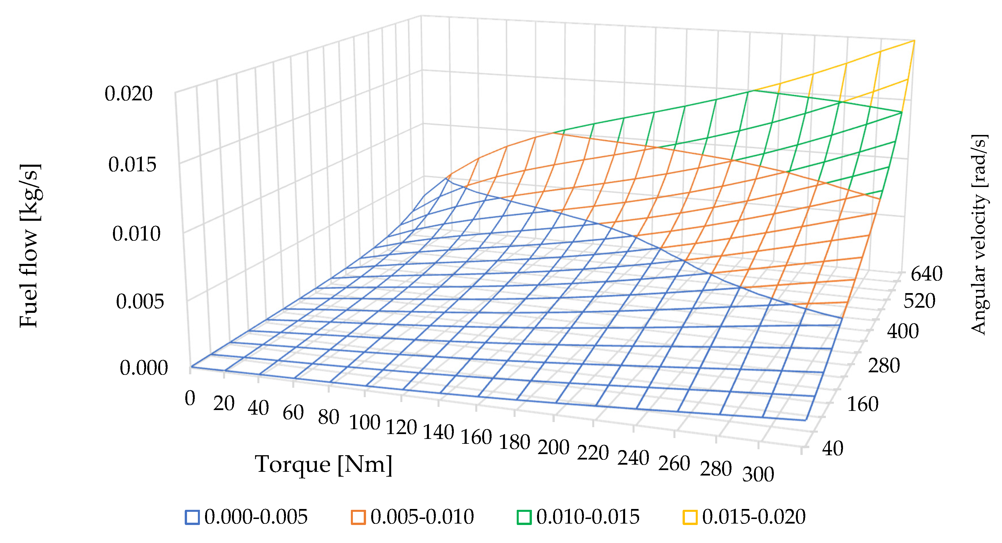
The calculation of instantaneous fuel mass demand uses the EPA’s published BTE characteristics for petrol 95. In the simulation model, it is assumed that for a certain point on the BTE characteristic (torque produced by the engine and engine operating speed), the algorithm calculates the required value of the instantaneous fuel flux based on its calorific value in such a way to provide the required energy demand. The efficiency of converting the energy contained in the fuel into mechanical work at a design point is the same for all fuels. No precise information was found in the literature on how changing the fuel mass affects the instantaneous efficiency of the engine at a given operating point.

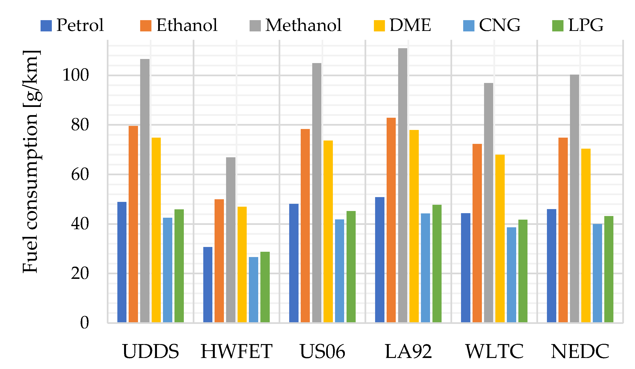
Figure 13 presents the results of the final consumption of tested fuels per one kilometer of travelled road for selected road tests. For petrol 95, the minimum value was obtained at the level of 30.64 g/km for the HWFET driving test, while the maximum value was obtained for LA92 (110.99 g/km) for methanol.

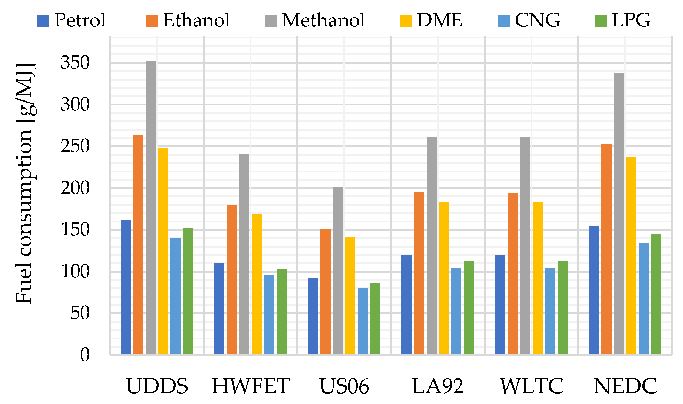
Figure 14 presents results of the simulator operation for the fuels under consideration and the driving tests in the form of the parameter of the final consumption of the tested fuels per 1 MJ of travelled road in the executed test. For CNG, the minimum value was achieved at the level of 80.4 g/MJ for the US 06 driving test, while the maximum value was obtained for methanol in the UDDS test (352.5 g/MJ).

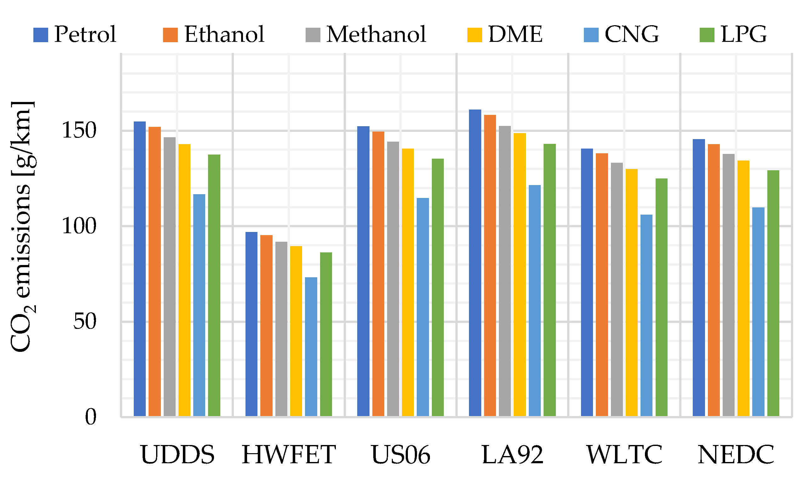
Below, in Figure 15, the data obtained from the simulations of driving tests with biofuels in the form of the parameter of the final CO₂ emission per kilometer travelled are summarized. For CNG, the minimum value was achieved at level of 97.7 g/km for the HWFET driving test, while the maximum value was obtained for LA92 (162.1 g/km).

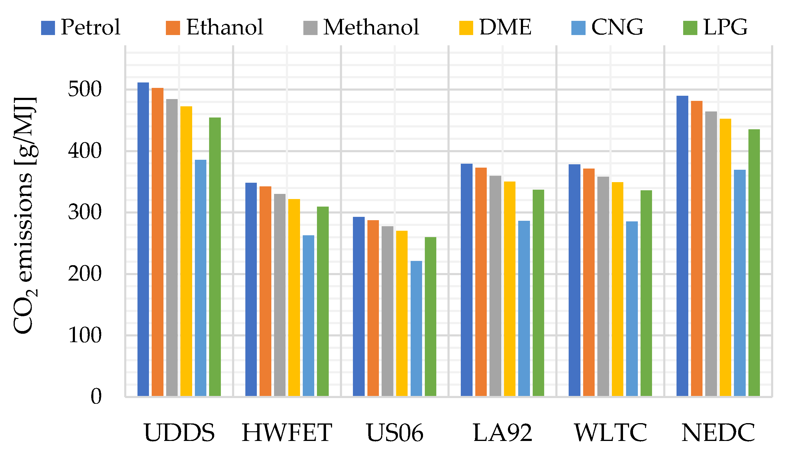
Figure 16 summarizes the simulator results for the considered fuels and driving tests in the form of the parameter of final CO₂ emission per 1 MJ. For petrol, the minimum value was achieved at the level of 338.7 g/MJ for the US 06 driving test, while the maximum value was obtained for UDDS (591.8 g/MJ).

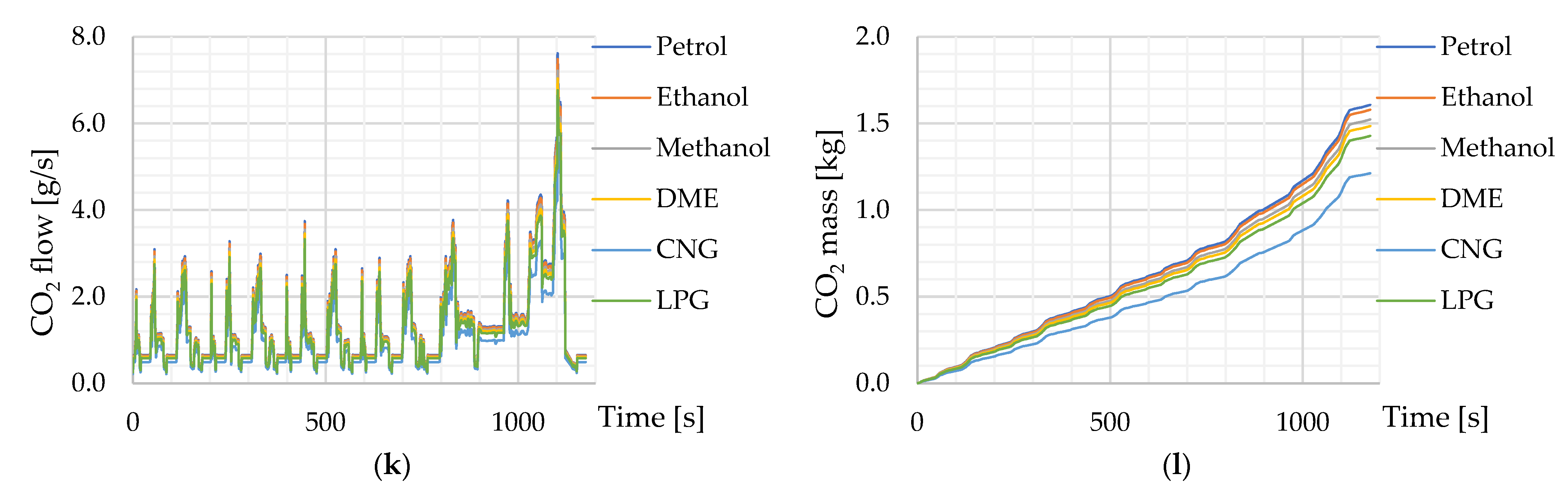
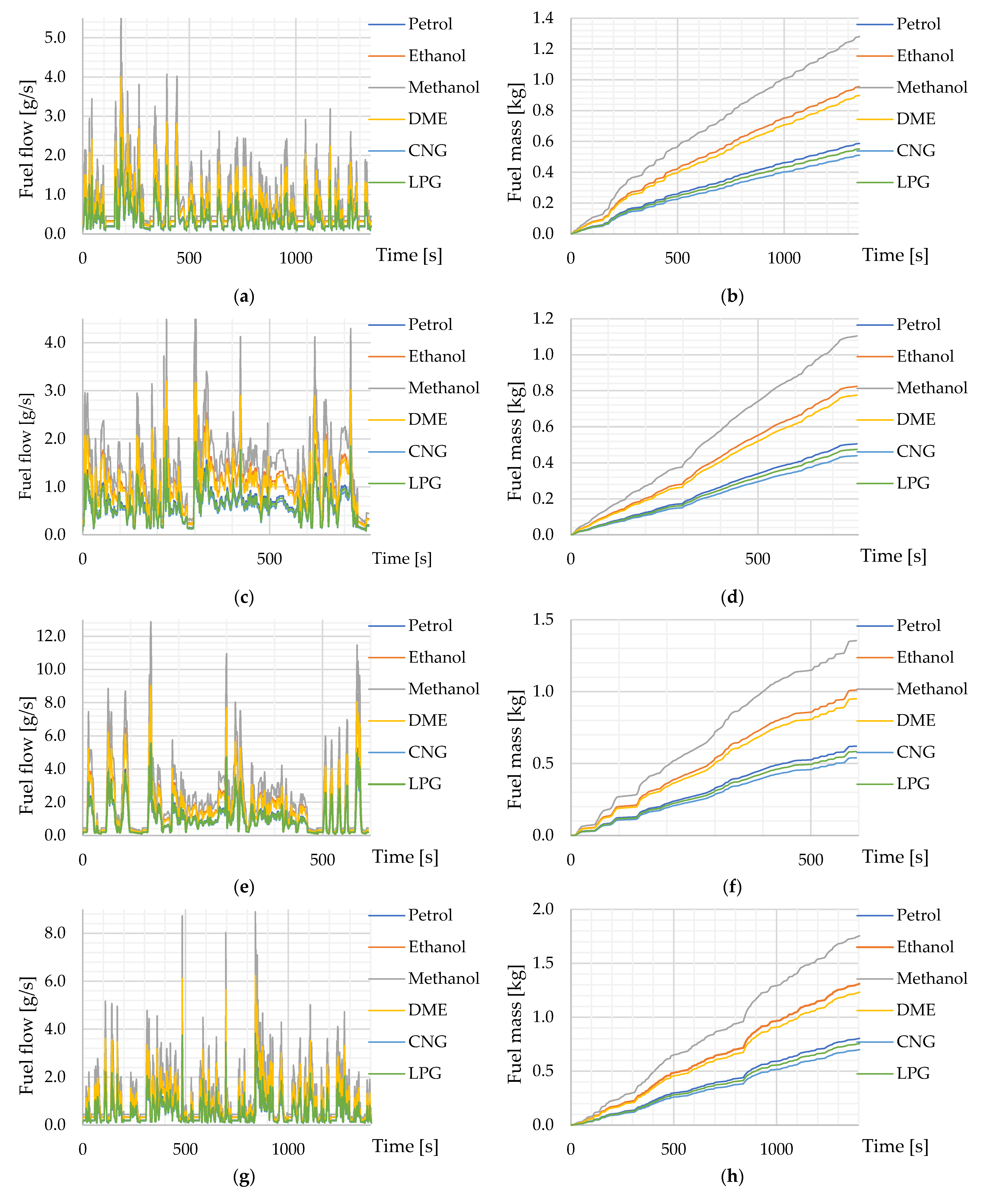
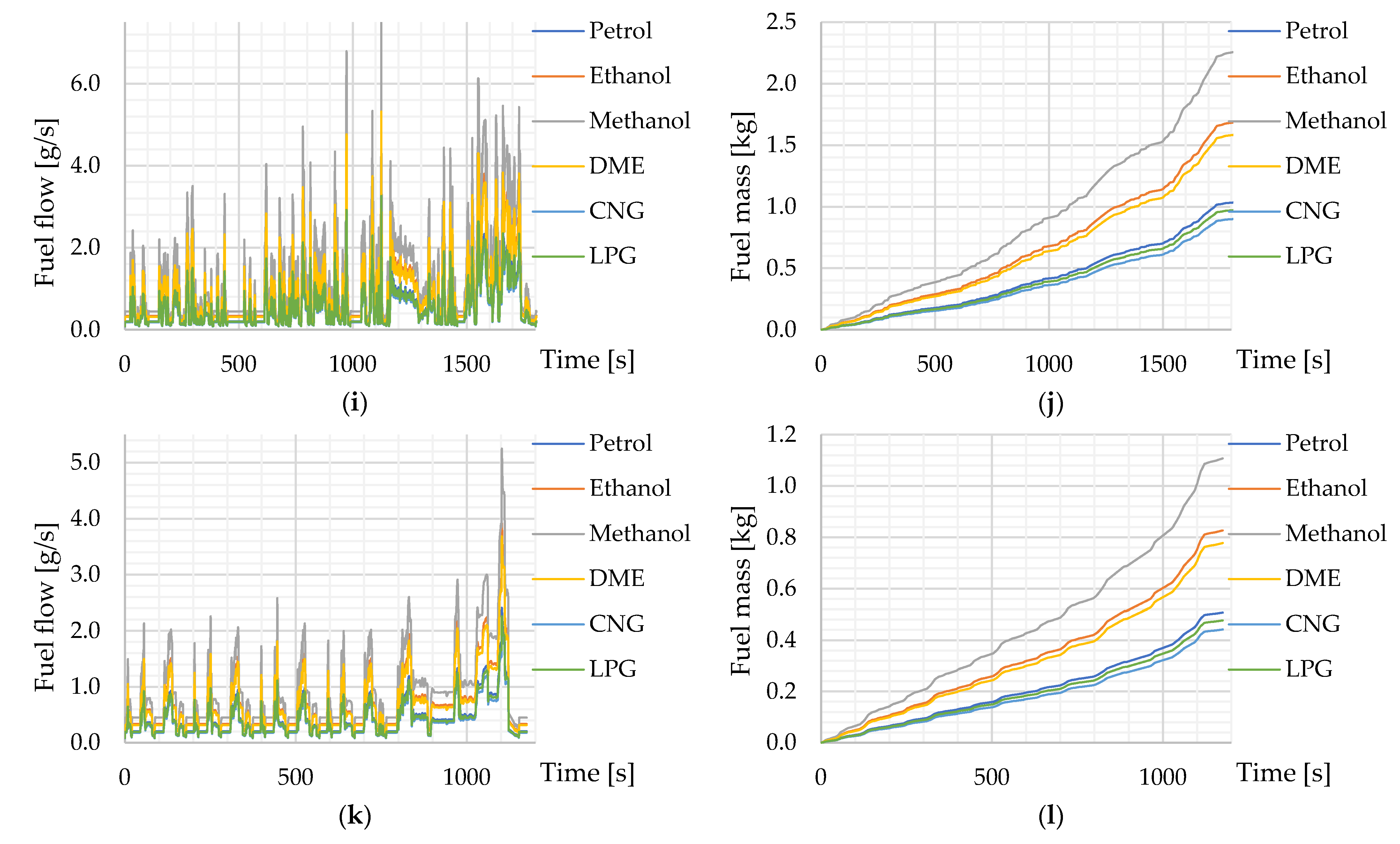
In the developed simulation model of CO₂ emissions in road tests, the BFC (specific fuel consumption) published by EPA data was based on engine testing for this engine model powered by petrol 95. In the further procedure, the BFC characteristics (EPA) were converted into fuel flux (kg/s), the values of which are presented in Figure 9, and were used in the simulation for the driving tests for fuel petrol 95. Then, for fuels other than gasoline 95 during the simulation operation, it was assumed that at a given instantaneous operation point of the engine (instantaneous torque on the crankshaft produced by the engine and the instantaneous value of the angular velocity of the crankshaft), an instantaneous energy flux of the value should be provided equal to fueling the engine with 95 petrol. The values of the consumption streams for fuels other than 95 gasoline have been computed on the basis of dependence (11). Big differences in the mass consumption of different fuels result from the large differences in the calorific value considered fuels (minimum methanol 19.93 MJ/kg, maximum CNG 50.0 MJ/kg).

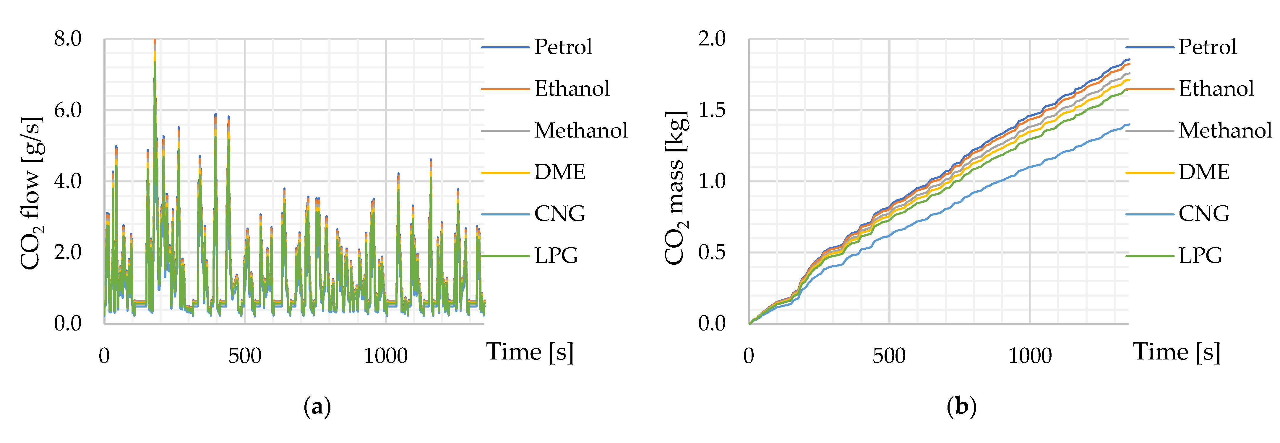
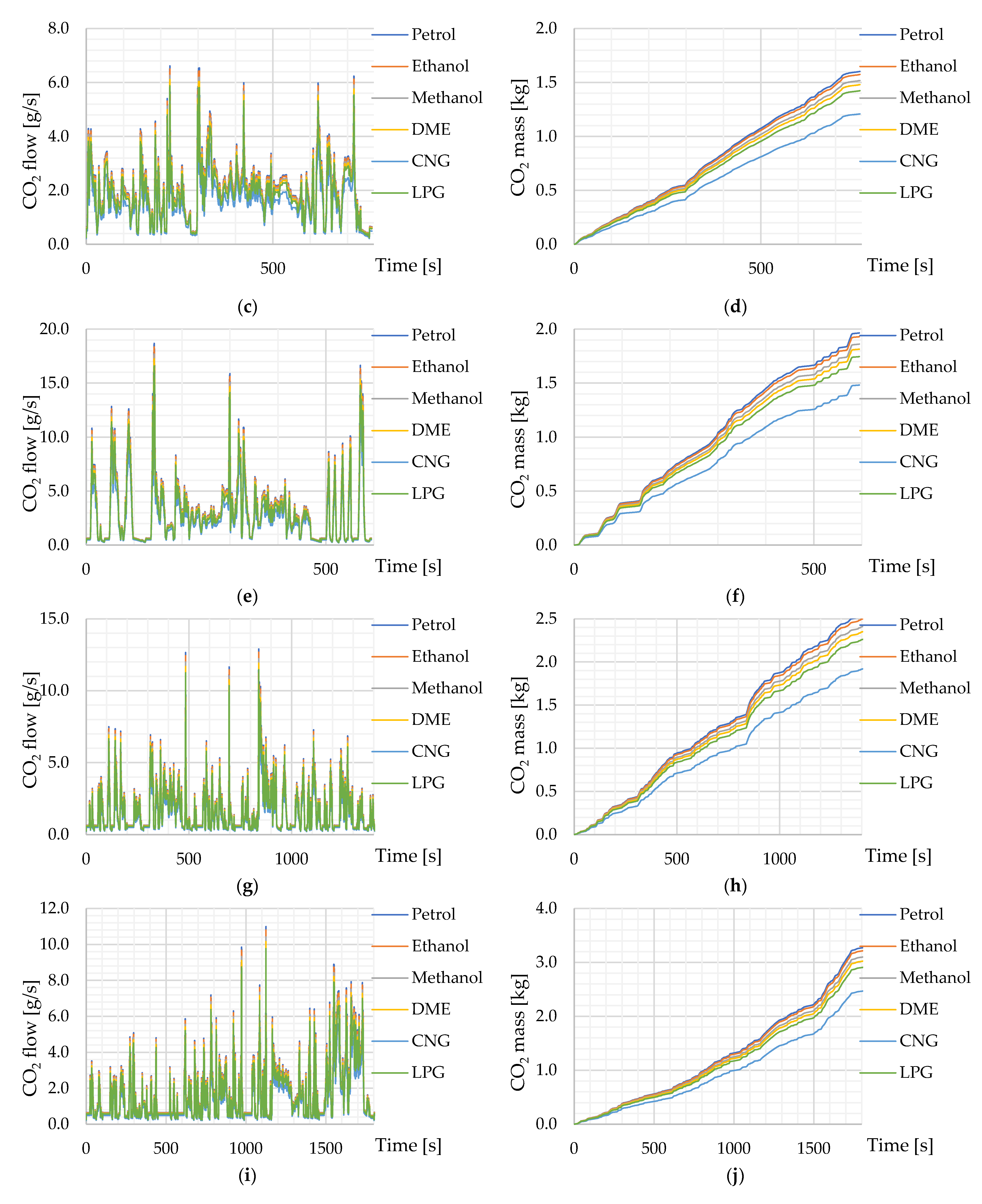
In the subsequent steps of the simulation basing on the mass fluxes obtained for the considered fuels, the CO₂ emissions were calculated. The final values of the CO₂ emission obtained from the simulation are shown in Figure 15. In turn, CO₂ emissions per kilometer of distance traveled by the vehicle showed much smaller differences. They confirmed the correctness of the calculations used in the developed simulation model.

5. Conclusions

The manuscript analyzes the possibility of using computer tools to simulate driving tests, the consumption of selected fuels and biofuels, and CO₂ emissivity. The analysis carried out was based on test results for the 2018 Toyota Camry LE vehicle obtained using a chassis dynamometer.

• The study analyzed six driving tests, differing in the speeds and accelerations achieved by the vehicle, the duration of the test, and the inclusion of vehicle accessories (e.g., air conditioning).
• Comparing the fuel consumption and CO₂ emission results from the driving test simulations and the available manufacturer’s values, it can be concluded that similar results were obtained for the NEDC driving test. This confirms that the vehicle in question has been approved under the NEDC test. Other tests were developed later and feature more dynamic load changes and the parameter of average vehicle engine load.
• Analyzing the final fuel consumption values for the real tests performed (EPA) and those obtained from the developed simulation of the 2018 Toyota Camry LE vehicle for selected road tests, the highest relative error occurred for the HWFET (3.018%).
• The highest energy efficiencies obtained from the 2018 Toyota Camry LE vehicle simulation for selected road tests were achieved for the US06 (0.249).
• Analyzing the parameter of the final consumption of tested fuels obtained from the simulations of the 2018 Toyota Camry LE vehicle for selected road tests, the highest values were achieved for the methanol fuel, for which the minimum value was achieved at the level of 1.105 kg for the HWFET driving test, while the maximum value was obtained in the WLTC test (2.257 kg). The lowest values of final consumption of tested fuels in the case of all of the analyzed driving tests were observed for the CNG fuel.
• Analyzing the parameter of the final consumption of tested fuels per kilometer travelled obtained from the simulations of the 2018 Toyota Camry LE vehicle for all of the analyzed driving tests, the lowest values were noticed for petrol 95 and CNG fuels. For the HWFET test, a value of 30.64 g/km was achieved for petrol 95 and 26.65 g/km for CNG. For WLTC, the final consumption of petrol 95 was 44.39 g/km and for CNG was 38.62 g/km.
• Analyzing the final consumption of tested fuels per 1 MJ obtained from the simulations of the 2018 Toyota Camry LE vehicle for the selected road tests, the highest consumption was noticed for methanol (in the UDDS test it was 52.5 g/MJ, and in the LA92 test it was 261.5 g/MJ).
• Analyzing the final CO₂ emissions obtained from the simulations of the 2018 Toyota Camry LE vehicle for the selected road tests, the highest values for all tested fuels were noticed for the WLTC test (petrol 3.274 kg, ethanol 3.217 kg, methanol 3.102 kg, DME 3.024 kg, LNG 2.909 kg, and CNG 2.469 kg).
• Considering the values of the final CO₂ emissions per kilometer travelled obtained from the simulations of the 2018 Toyota Camry LE vehicle for the selected road tests, the highest value was recorded for petrol in the LA92 test with 161.0 g/km and the lowest for CNG in the HWFET test with 73.1 g/km.
• For the parameter of carbon dioxide emission per unit of energy produced (1 MJ), maximum values were obtained for UDDS petrol (511.3 g/MJ), ethanol (502.4 g/MJ), methanol (484.4 g/MJ), DME (472.3 g/kMJ), and CNG (385.6 g/MJ).
• The developed computer tool using OpenModelica computer software can support the development of a method to identify selected aspects of operating conditions and can be used to assess the energy efficiency of automotive vehicles with spark-ignition engines fueled with fuels and biofuels.
• Due to its open source code, Open Modelica has a lot of potential for modifications in the library package to extend its functionality. Commercial packages are closed and have no such modification capabilities.

References

1. Legutko, S. Development trends in machines operation maintenance. Eksploat. I Niezawodn. Maint. Reliab. 2009, 2, 8–16. [Google Scholar]
2. Saeed, N.A.; Mahrous, E.; Abouel Nasr, E.; Awrejcewicz, J. Nonlinear Dynamics and Motion Bifurcations of the Rotor Active Magnetic Bearings System with a New Control Scheme and Rub-Impact Force. Symmetry 2021, 13, 1502. [Google Scholar] [CrossRef]
3. Prażnowski, K.; Mamala, J. Problems in Assessing Pneumatic Wheel Unbalance of a Passenger Car Determined with Test Road in Normal Conditions. SAE Technical Paper 2017. [Google Scholar] [CrossRef]
4. Piwowar, A.; Dzikuć, M. Development of Renewable Energy Sources in the Context of Threats Resulting from Low-Altitude Emissions in Rural Areas in Poland: A Review. Energies 2019, 12, 3558. [Google Scholar] [CrossRef] [Green Version]
5. Tutak, M.; Brodny, J.; Bindzár, P. Assessing the Level of Energy and Climate Sustainability in the European Union Countries in the Context of the European Green Deal Strategy and Agenda 2030. Energies 2021, 14, 1767. [Google Scholar] [CrossRef]
6. Daziano, R.; Waygood, E.O.D.; Patterson, Z.; Feinberg, M.; Wang, B. Reframing greenhouse gas emissions information presentation on the Environmental Protection Agency’s new-vehicle labels to increase willingness to pay. J. Clean. Prod. 2021, 279, 123669. [Google Scholar] [CrossRef]
7. Miyamoto, M.; Takeuchi, K. Climate agreement and technology diffusion: Impact of the Kyoto Protocol on international patent applications for renewable energy technologies. Energy Policy 2019, 129, 1331–1338. [Google Scholar] [CrossRef] [Green Version]
8. Gunfaus, M.T.; Waisman, H. Assessing the adequacy of the global response to the Paris Agreement: Toward a full appraisal of climate ambition and action. Earth Syst. Gov. 2021, 8, 100102. [Google Scholar] [CrossRef]
9. Ortega-Cabezas, P.M.; Colmenar-Santos, A.; Borge-Diez, D.; Blanes-Peiró, J.J. Can Eco-routing, Eco-driving and Eco-charging Contribute to the European Green Deal? Energy 2021, 228, 120532. [Google Scholar] [CrossRef]
10. Capros, C.; Kannavou, M.; Evangelopoulou, S.; Petropoulos, A.; Siskos, P.; Tasios, N.; Zazias, G.; DeVita, A. Outlook of the EU energy system up to 2050: The case of scenarios prepared for European Commission’s “clean energy for all Europeans” package using the PRIMES model. Energy Strategy Rev. 2018, 22, 255–263. [Google Scholar] [CrossRef]
11. Sustainable and Smart Mobility Strategy—Putting European Transport on Track for the Future. Available online: https://ec.europa.eu/transport/sites/transport/files/legislation/com20200789.pdf (accessed on 12 April 2021).
12. Cepeliauskaite, G.; Keppner, B.; Simkute, Z.; Stasiskiene, Z.; Leuser, L.; Kalnina, I.; Kotovica, N.; Andiņš, J.; Muiste, M. Smart-Mobility Services for Climate Mitigation in Urban Areas: Case Studies of Baltic Countries and Germany. Sustainability 2021, 13, 4127. [Google Scholar] [CrossRef]
13. Economic and Market Reports. Available online: https://www.acea.be/statistics/tag/category/economic-and-market-outlook (accessed on 12 April 2021).
14. Fuel Types of New Passenger Cars. Available online: https://www.acea.be/statistics/tag/category/share-of-diesel-in-new-passenger-cars (accessed on 12 April 2021).
15. Tucki, K.; Orynycz, O.; Mitoraj-Wojtanek, M. Perspectives for Mitigation of CO2 Emission due to Development of Electromobility in Several Countries. Energies 2020, 13, 4127. [Google Scholar] [CrossRef]
16. Haas, T.; Sander, H. Decarbonizing Transport in the European Union: Emission Performance Standards and the Perspectives for a European Green Deal. Sustainability 2020, 12, 8381. [Google Scholar] [CrossRef]
17. Development of the Methodology and Estimation of the External Costs of Air Pollution Emitted from Road transport at National Level. Available online: https://stat.gov.pl/download/gfx/portalinformacyjny/pl/defaultstronaopisowa/6150/1/1/raport_koszty_zewnetrzne_emisji_zanieczyszczen.pdf (accessed on 12 April 2021).
18. García, A.; Monsalve-Serrano, J.; Sari, R.L.; Tripathi, S. Pathways to achieve future CO2 emission reduction targets for bus transit networks. Energy 2022, 244, 123177. [Google Scholar] [CrossRef]
19. All about CO2 Emissions Regulations & VECTO. Available online: https://www.continental-tires.com/transport/fleetsolutions/co2-regulations-vecto (accessed on 12 April 2021).
20. Bielaczyc, P.; Woodburn, J. Trends in Automotive Emission Legislation: Impact on LD Engine Development. Fuels. Lubricants and Test Methods: A Global View with a Focus on WLTP and RDE Regulations. Emiss. Control Sci. Technol. 2019, 5, 86–98. [Google Scholar] [CrossRef] [Green Version]
21. Jaworski, A.; Mądziel, M.; Lew, K.; Campisi, T.; Woś, P.; Kuszewski, H.; Wojewoda, P.; Ustrzycki, A.; Balawender, K.; Jakubowski, M. Evaluation of the Effect of Chassis Dynamometer Load Setting on CO2 Emissions and Energy Demand of a Full Hybrid Vehicle. Energies 2022, 15, 122. [Google Scholar] [CrossRef]
22. Scope and Manner of Technical Testing of Vehicles and Model Documents Used for These Tests. Available online: https://sip.lex.pl/akty-prawne/dzu-dziennik-ustaw/zakres-i-sposob-przeprowadzania-badan-technicznych-pojazdow-oraz-wzory-17568864 (accessed on 12 April 2021).
23. Study on the EU Harmonisation of the Requirements for the Road Circulation of Mobile Machinery–FWC ENTR/172/PP/2012/FC/Lot1. Final Report. Available online: https://ec.europa.eu/docsroom/documents/17786/attachments/1/translations/en/renditions/native (accessed on 12 April 2021).
24. Cha, J.; Lee, J.; Chon, M.S. Evaluation of real driving emissions for Euro 6 light-duty diesel vehicles equipped with LNT and SCR on domestic sales in Korea. Atmos. Environ. 2019, 196, 133–142. [Google Scholar] [CrossRef]
25. Triantafyllopoulos, G.; Dimaratos, A.; Ntziachristos, L.; Bernard, Y.; Dornoff, J.; Samaras, Z. A study on the CO2 and NOx emissions performance of Euro 6 diesel vehicles under various chassis dynamometer and on-road conditions including latest regulatory provisions. Sci. Total Environ. 2019, 666, 337–346. [Google Scholar] [CrossRef]
26. Chen, L.; Wang, Z.; Liu, S.; Qu, L. Using a chassis dynamometer to determine the influencing factors for the emissions of Euro VI vehicles. Transp. Res. Part D Transp. Environ. 2018, 65, 564–573. [Google Scholar] [CrossRef]
27. Duarte, G.O.; Gonçalves, G.A.; Farias, T.L. Analysis of fuel consumption and pollutant emissions of regulated and alternative driving cycles based on real-world measurements. Transp. Res. Part D Transp. Environ. 2016, 44, 43–54. [Google Scholar] [CrossRef]
28. García-Contreras, R.; Soriano, J.A.; Fernández-Yáñez, P.; Sánchez-Rodríguez, L.; Mata, C.; Gómez, A.; Armas, O.; Cárdenas, M.D. Impact of regulated pollutant emissions of Euro 6d-Temp light-duty diesel vehicles under real driving conditions. J. Clean. Prod. 2021, 286, 124927. [Google Scholar] [CrossRef]
29. Myung, C.L.; Choi, K.; Kim, J.; Lim, Y.; Lee, J.; Park, S. Comparative study of regulated and unregulated toxic emissions characteristics from a spark ignition direct injection light-duty vehicle fueled with gasoline and liquid phase LPG (liquefied petroleum gas). Energy 2012, 44, 189–196. [Google Scholar] [CrossRef]
30. Continental. Worldwide Emission Standards and Related Regulations. Passenger Cars/Light and Medium Duty Vehicles May 2019. Available online: https://www.continental-automotive.com/getattachment/8f2dedad-b510-4672-a005-3156f77d1f85/EMISSIONBOOKLET2019.pdf (accessed on 12 April 2021).
31. Merkisz, J.; Pielecha, J.; Molik, P. Analysis of vehicle working conditions in the homologation tests. Logistyka 2015, 3, 3220–3227. [Google Scholar]
32. Emissions in the Automotive Sector. Available online: https://ec.europa.eu/growth/sectors/automotive/environment-protection/emissions_en (accessed on 12 April 2021).
33. Kooijman, D.G.; Balau, A.E.; Wilkins, S.; Ligterink, N.; Cuelenaere, R. WLTP Random Cycle Generator. In Proceedings of the 12th IEEE Vehicle Power and Propulsion Conference (VPPC 2015), Montreal, QC, Canada, 19–22 October 2015; ISBN 9781467376372. [Google Scholar]
34. Tsiakmakis, S.; Fontaras, G.; Anagnostopoulos, K.; Ciuffo, B.; Pavlovic, J.; Marotta, A. A simulation based approach for quantifying CO2 emissions of light duty vehicle fleets. A case study on WLTP introduction. Transp. Res. Procedia 2017, 25, 3898–3908. [Google Scholar] [CrossRef]
35. Blanco-Rodriguez, D.; Vagnoni, G.; Holderbaum, B. EU6 C-Segment Diesel vehicles, a challenging segment to meet RDE and WLTP requirements. IFAC-PapersOnLine 2016, 49, 649–656. [Google Scholar] [CrossRef]
36. Triantafyllopoulos, G.; Katsaounis, D.; Karamitros, D.; Ntziachristos, L.; Samaras, Z. Experimental assessment of the potential to decrease diesel NOx emissions beyond minimum requirements for Euro 6 Real Drive Emissions (RDE) compliance. Sci. Total Environ. 2018, 618, 1400–1407. [Google Scholar] [CrossRef] [PubMed]
37. Dimaratos, A.; Tsokolis, D.; Fontaras, G.; Tsiakmakis, S.; Ciuffo, B.; Samaras, Z. Comparative Evaluation of the Effect of Various Technologies on Light-duty Vehicle CO2 Emissions over NEDC and WLTP. Transp. Res. Procedia 2016, 14, 3169–3178. [Google Scholar] [CrossRef] [Green Version]
38. Massaguer, E.; Massaguer, A.; Pujol, T.; Comamala, M.; Montoro, L.; Gonzalez, J.R. Fuel economy analysis under a WLTP cycle on a mid-size vehicle equipped with a thermoelectric energy recovery system. Energy 2019, 179, 306–314. [Google Scholar] [CrossRef]
39. Chłopek, Z. Synthesis of driving cycles in accordance with the criterion of similarity of frequency characteristics. Eksploat. I Niezawodn. Maint. Reliab. 2016, 18, 572–577. [Google Scholar] [CrossRef]
40. Demuynck, J.; Bosteels, D.; Paepe, M.D.; Favre, C.; May, J.; Verhelst, S. Recommendations for the new WLTP cycle based on an analysis of vehicle emission measurements on NEDC and CADC. Energy Policy 2012, 49, 234–242. [Google Scholar] [CrossRef] [Green Version]
41. May, J.; Bosteels, D.; Favre, C. An Assessment of Emissions from Light-Duty Vehicles using PEMS and Chassis Dynamometer Testing. SAE 2014, 7, 1326–1335. [Google Scholar] [CrossRef] [Green Version]
42. May, J.; Favre, C.; Bosteels, D.; Andersson, J.; Clarke, D.; Heaney, M. On-Road Testing and PEMS Data Analysis for Two Euro 6 Diesel Vehicles. Available online: http://www.aecc.eu/wp-content/uploads/2016/08/140918-AECC-paper-on-RDE-TAP-Conference-Graz.pdf (accessed on 12 April 2021).
43. From NEDC to WLTP: What Will Change? Available online: https://www.wltpfacts.eu/from-nedc-to-wltp-change/ (accessed on 27 November 2021).
44. Karagöz, Y. Analysis of the impact of gasoline. Biogas and biogas + hydrogen fuels on emissions and vehicle performance in the WLTC and NEDC. Int. J. Hydrogen Energy 2019, 44, 31621–31632. [Google Scholar] [CrossRef]
45. EPA Federal Test Procedure (FTP). Available online: https://www.epa.gov/emission-standards-reference-guide/epa-federal-test-procedure-ftp (accessed on 12 April 2021).
46. EPA Highway Fuel Economy Test Cycle (HWFET). Available online: https://dieselnet.com/standards/cycles/hwfet.php (accessed on 12 April 2021).
47. Merkisz, J.; Pielecha, J.; Pachołek, A. Directions of on board diagnostic system development in passenger cars. J. Konbin 2008, 1, 165–185. [Google Scholar] [CrossRef]
48. Rahman, S.M.A.; Fattah, I.M.R.; Ong, H.C.; Ashik, F.R.; Hassan, M.M.; Murshed, M.T.; Imran, M.A.; Rahman, M.H.; Rahman, M.A.; Hasan, M.A.M.; et al. State-of-the-Art of Establishing Test Procedures for Real Driving Gaseous Emissions from Light- and Heavy-Duty Vehicles. Energies 2021, 14, 4195. [Google Scholar] [CrossRef]
49. Chłopek, Z. The modeling basis of the pollutant emission and the fuel and energy consumption for internal combustion engines of motor vehicles. Combust. Engines 2015, 162, 177–185. [Google Scholar]
50. SFTP Cycle Contributionsto Light-Duty Diesel Exhaust Emissions. Available online: https://apps.dtic.mil/dtic/tr/fulltext/u2/a402903.pdf (accessed on 12 April 2021).
51. Jenn, A.; Azevedo, I.L.; Michalek, J.J. Alternative-fuel-vehicle policy interactions increase U.S. greenhouse gas emissions. Transp. Res. Part A Policy Pract. 2019, 124, 396–407. [Google Scholar] [CrossRef] [Green Version]
52. Kang, S.; Min, K. Dynamic simulation of a fuel cell hybrid vehicle during the federal test procedure-75 driving cycle. Appl. Energy 2016, 161, 181–196. [Google Scholar] [CrossRef]
53. US: Light-duty: Highway Fuel Economy Cycle (HWFET). Available online: https://www.transportpolicy.net/standard/us-light-duty-highway-fuel-economy-cycle-hwfet/ (accessed on 12 April 2021).
54. Eckert, J.J.; Santiciolli, F.M.; Silva, L.C.A.; Dedini, F.G. Vehicle drivetrain design multi-objective optimization. Mech. Mach. Theory 2021, 156, 104123. [Google Scholar] [CrossRef]
55. US: Light-Duty: Emissions. Available online: https://www.transportpolicy.net/standard/us-light-duty-emissions/ (accessed on 12 November 2021).
56. Khalfi, J.; Boumaaz, N.; Soulmani, A.; Laadissi, E.M. Box–Jenkins Black-Box Modeling of a Lithium-Ion Battery Cell Based on Automotive Drive Cycle Data. World Electr. Veh. J. 2021, 12, 102. [Google Scholar] [CrossRef]
57. Pałuchowska, M.; Jakóbiec, J. The quality specification of E10 engine petrol. Naft. Gaz 2011, 67, 825–830. [Google Scholar]
58. Speight, J.G.; El-Gendy, N.S. Refinery Products and By-Products. In Introduction to Petroleum Biotechnology, 1st ed.; Speight, J.G., El-Gendy, N.S., Eds.; Gulf Professional Publishing: Oxford, UK, 2010; pp. 41–68. [Google Scholar]
59. Kim, J.; Kim, K.; Oh, S. An assessment of the ultra-lean combustion direct-injection LPG (liquefied petroleum gas) engine for passenger-car applications under the FTP-75 mode. Fuel Processing Technol. 2016, 154, 219–226. [Google Scholar] [CrossRef]
60. Caban, J.; Voltr, O. A Study on the use of eco-driving technique in city traffic. Arch. Automot. Eng. Arch. Motoryz. 2021, 93, 15–25. [Google Scholar] [CrossRef]
61. Time for Methane? Alternative Fuels: CNG and LNG under the Loupe. Available online: http://www.ekspert-flotowy.pl/artykuly/552/czas-na-metan-paliwa-alternatywne-cng-i-lng-pod-lupa.html (accessed on 6 February 2021).
62. Suarez-Bertoa, R.; Pechout, M.; Vojtíšek, M.; Astorga, C. Regulated and Non-Regulated Emissions from Euro 6 Diesel. Gasoline and CNG Vehicles under Real-World Driving Conditions. Atmosphere 2020, 11, 204. [Google Scholar] [CrossRef] [Green Version]
63. Brzeżański, M. Carbon dioxide emissions in the aspect of applied engine fuels. Combust. Engines 2007, 131, 62–67. [Google Scholar] [CrossRef]
64. Methanol as an Alternative Transportation Fuel in the US: Options for Sustainable and/or Energy-Secure Transportation. Available online: https://afdc.energy.gov/files/pdfs/mit_methanol_white_paper.pdf (accessed on 12 April 2021).
65. Prażnowski, K.; Bieniek, A.; Mamala, J.; Deptuła, A. The Use of Multicriteria Inference Method to Identify and Classify Selected Combustion Engine Malfunctions Based on Vehicle Structure Vibrations. Sensors 2021, 21, 2470. [Google Scholar] [CrossRef]
66. Żółty, M.; Stępień, Z. Ethanol fuels for spark ignition engines. Naft. Gaz 2016, 72, 761–769. [Google Scholar] [CrossRef]
67. Pałuchowska, M.; Jakóbiec, J. Effects of ethanol addition and chemical composition of the fuel on its performance parameters. Autobusy Tech. Eksploat. Syst. Transp. 2012, 13, 140–149. [Google Scholar]
68. Zhang, Q.; Qian, X.; Fu, L.; Yuan, M.; Chen, Y. Shock wave evolution and overpressure hazards in partly premixed gas deflagration of DME/LPG blended multi-clean fuel. Fuel 2020, 268, 117368. [Google Scholar] [CrossRef]
69. Fabiś, P.; Flekiewicz, B. Influence of LPG and DME Composition on Spark Ignition Engine Performance. Energies 2021, 14, 5583. [Google Scholar] [CrossRef]
70. Georgios, Z.N.; Alessandro, T.; Ignacio, P.R.; Theodoros, G.; Georgios, F. A generalized component efficiency and input-data generation model for creating fleet-representative vehicle simulation cases in VECTO. SAE 2019. [Google Scholar] [CrossRef] [Green Version]
71. Analysis of VECTO Data for Heavy-Duty Vehicles (HDV) CO2 Emission Targets. Available online: https://ec.europa,eu/jrc/en/publication/eur-scientific-and-technical-research-reports/analysis-vecto-data-heavy-duty-vehicles-hdv-co2-emission-targets (accessed on 15 January 2021).
72. CO2MPAS: Vehicle Simulator Predicting NEDC CO2 Emissions from WLTP. Available online: https://co2mpas.io/ (accessed on 15 February 2021).
73. Mogno, C.; Fontaras, G.; Arcidiacono, V.; Komnos, D.; Pavlovic, J.; Ciuffo, B.; Makridis, M.; Valverde, V. The application of the CO2MPAS model for vehicle CO2 emissions estimation over real traffic conditions. Transp. Policy, 2020; in press. [Google Scholar] [CrossRef]
74. López-Martínez, J.M.; Jiménez, F.; Páez-Ayuso, F.J.; Flores-Holgado, M.N.; Arenas, A.N.; Arenas-Ramirez, B.; Aparicio-Izquierdo, F. Modelling the fuel consumption and pollutant emissions of the urban bus fleet of the city of Madrid. Transp. Res. Part D Transp. Environ. 2017, 52, 112–127. [Google Scholar] [CrossRef]
75. 2018 Toyota Camry LE Vehicle Tier 2 Fuel—Test Data Package. Dated 07-30-20. Ann Arbor. MI: US EPA. National Vehicle and Fuel Emissions Laboratory. National Center for Advanced Technology. Available online: https://www.epa.gov/vehicle-and-fuel-emissions-testing/benchmarking-advanced-low-emission-light-duty-vehicle-technology (accessed on 27 November 2021).
76. Moskalik, A.; Stuhldreher, M.; Kargul, J. Benchmarking a 2018 Toyota Camry UB80E Eight-Speed Automatic Transmission. SAE 2020. Available online: https://www.epa.gov/sites/production/files/2020-05/documents/sae-2020-01-1286-benchmark-2018-toyota-camry-ub80e-eight-speed-auto-trans.pdf (accessed on 27 November 2021). [CrossRef]
77. Dynamometer Drive Schedules. Available online: https://www.epa.gov/vehicle-and-fuel-emissions-testing/dynamometer-drive-schedules (accessed on 27 November 2021).
78. Fredette, D.; Pavlich, C.; Ozguner, U. Development of a UDDS-Comparable Framework for the Assessment of Connected and Automated Vehicle Fuel Saving Techniques. IFAC-PapersOnLine 2015, 48, 306–312. [Google Scholar] [CrossRef]
79. Daemme, L.C.; Penteado, R.; Ferreira, R.S.; Errera, M.R.; Corrêa, S.M.; Ostapiuk, I.F. Particulate matter emissions from flex-fuel vehicles with direct fuel injection. Atmos. Pollut. Res. 2021, 12, 101078. [Google Scholar] [CrossRef]
80. EPA US06 or Supplemental Federal Test Procedure (SFTP). Available online: https://www.epa.gov/emission-standards-reference-guide/epa-us06-or-supplemental-federal-test-procedure-sftp (accessed on 27 November 2021).
81. Kazemiparkouhi, F.; Falconi, T.M.A.; MacIntosh, D.L.; Clark, N. Comprehensive US database and model for ethanol blend effects on regulated tailpipe emissions. Sci. Total Environ. 2021, 812, 151426. [Google Scholar] [CrossRef]
82. Shen, K.; Chang, I.; Chen, H.; Zhang, Z.; Wang, B.; Wang, Y. Experimental study on the effects of exhaust heat recovery system (EHRS) on vehicle fuel economy and emissions under cold start new European driving cycle (NEDC). Energy Convers. Manag. 2019, 197, 111893. [Google Scholar] [CrossRef]
83. Ko, J.; Jin, D.; Jang, W.; Myung, C.L.; Kwon, S.; Park, S. Comparative investigation of NOx emission characteristics from a Euro 6-compliant diesel passenger car over the NEDC and WLTC at various ambient temperatures. Appl. Energy 2017, 187, 652–662. [Google Scholar] [CrossRef]
84. Addendum15: Global Technical Regulation No. 15. Worldwide Harmonized Light Vehicles Test Procedure. Available online: https://unece.org/fileadmin/DAM/trans/main/wp29/wp29r-1998agr-rules/ECE-TRANS-180a15e.pdf (accessed on 27 November 2021).
85. Giechaskiel, B.; Suarez-Bertoa, R.; Lähde, T.; Clairotte, M.; Carriero, M.; Bonnel, P.; Maggiore, M. Evaluation of NOx emissions of a retrofitted Euro 5 passenger car for the Horizon prize “Engine retrofit”. Environ. Res. 2018, 166, 298–309. [Google Scholar] [CrossRef]
86. Suarez-Bertoa, R.; Zardini, A.A.; Lilova, V.; Meyer, D.; Nakatani, S.; Hibel, F.; Ewers, J.; Clairotte, M.; Hill, L.; Astorga, C. Intercomparison of real-time tailpipe ammonia measurements from vehicles tested over the new world-harmonized light-duty vehicle test cycle (WLTC). Environ. Sci. Pollut. Res. 2015, 22, 7450–7460. [Google Scholar] [CrossRef] [Green Version]
87. Kordylewski, W. Spalanie i Paliwa, 5th ed.; Oficyna Wydawnicza Politechniki Wrocławskiej: Wrocław, Poland, 2008; pp. 10–470. ISBN 978-83-7493-378-0. [Google Scholar]
88. Dobras, S.; Więcław-Solny, L.; Chwoła, T.; Krótki, A.; Wilk, A.; Tatarczuk, A. Renewable methanol as a fuel and feedstock in the chemical industry. Zesz. Nauk. Inst. Gospod. Surowcami Miner. Energią PAN 2017, 98, 27–37. [Google Scholar]
89. Gwardiak, H.; Rozycki, K.; Ruszkarska, M.; Tylus, J.; Walisiewicz-Niedbalska, W. Evaluation of fatty acid methyl esters (FAME) obtained from various feedstock. Rośliny Oleiste-Oilseed Crops 2011, 32, 137–147. [Google Scholar]
90. Piątkowski, P.; Bohdal, T. Testing of Ecological Properties of Spark Ignition Engine Fed with LPG Mixture. Rocz. Ochr. Sr. (Annu. Set Environ. Prot.) 2011, 13, 607–618. [Google Scholar]
91. The 2020 EPA Automotive Trends Report: Greenhouse Gas Emissions, Fuel Economy, and Technology since 1975. Available online: https://www.epa.gov/automotive-trends/download-automotive-trends-report#Full%20Report (accessed on 30 November 2021).
Figure 1. General diagram of the developed driving test simulation for the 2018 Toyota Camry LE vehicle.
Energies 15 00995 g001
Figure 2. Waveform of instantaneous values [75]: (a) torque losses as a function of engine crankshaft angular velocity of the 2018 Toyota Camry LE vehicle; (b) maximum engine crankshaft torque as a function of engine angular velocity of the 2018 Toyota Camry LE vehicle.
Energies 15 00995 g002
Figure 3. Diagram of the “engine” module in the developed test simulation.
Energies 15 00995 g003
Figure 4. Waveform of values [74]: (a) K-factor as a function of speed ratio ν; (b) conversion ratio μ as a function of speed ratio ν.
Energies 15 00995 g004
Figure 5. Diagram of the “torque converter” module in the developed test simulation.
Energies 15 00995 g005
Figure 6. Waveform of transmission torque loss variations as a function of the input shaft torque and gear ratio value [75].
Energies 15 00995 g006
Figure 7. Diagram of the “drivetrain” module in the developed test simulation.
Energies 15 00995 g007
Figure 8. Diagram of the “vehicle” module in the developed test simulation.
Energies 15 00995 g008
Figure 9. Waveform of the instantaneous values of the fuel stream consumed by the engine as a function of the engine crankshaft angular velocity and torque generated at the engine crankshaft [75].
Energies 15 00995 g009
Figure 10. 2018 Toyota Camry LE—waveforms of instantaneous values: (a) vehicle speed obtained from the simulation of selected road tests; (b) distance travelled by the vehicle obtained from simulation of selected road tests; (c) angular velocity of the crankshaft of the vehicle engine obtained from simulation of selected road tests; (d) torque produced at the crankshaft by the vehicle engine obtained from simulation of selected road tests; (e) power generated by the engine obtained from simulation of selected road tests; (f) mechanical energy generated by the vehicle engine obtained from simulation of selected road tests; (g) power lost in the vehicle drivetrain obtained from simulation of selected road tests; (h) energy lost in the vehicle transmission obtained from simulation of selected road tests; (i) power lost in the braking system of the 2018 Toyota Camry LE vehicle obtained from simulation of selected road tests; (j) energy lost in the vehicle braking system obtained from simulation of selected road tests; (k) power lost by vehicle rolling resistance forces obtained from simulation of selected road tests; (l) energy lost by vehicle rolling resistance forces obtained from simulation of selected road tests; (m) power delivered in the vehicle fuel stream obtained from simulation of selected road tests; (n) energy delivered in the fuel stream of the 2018 Toyota Camry LE vehicle obtained from simulation of selected road tests.
Energies 15 00995 g010aEnergies 15 00995 g010bEnergies 15 00995 g010c
Figure 11. 2018 Toyota Camry LE—waveforms of instantaneous values: (a) vehicle engine fuel stream obtained from UDDS road test simulation for selected fuels; (b) fuel consumption obtained from UDDS road test simulation for selected fuels; (c) vehicle engine fuel stream obtained from HWFET road test simulation for selected fuels; (d) vehicle fuel consumption obtained from HWFET road test simulation for selected fuels; (e) vehicle engine fuel stream obtained from US06 road test simulation for selected fuels; (f) vehicle fuel consumption obtained from US06 road test simulation for selected fuels; (g) the vehicle engine fuel flow obtained from LA92 road test simulation for selected fuels; (h) vehicle fuel consumption obtained from LA92 road test simulation for selected fuels; (i) the vehicle engine fuel flow obtained from WLTC road test simulation for selected fuels; (j) vehicle fuel consumption obtained from simulation of WLTC road test for selected fuels; (k) vehicle engine fuel flow obtained from simulation of NEDC road test for selected fuels; (l) vehicle fuel consumption obtained from simulation of NEDC road test for selected fuels.
Energies 15 00995 g011aEnergies 15 00995 g011b
Figure 12. 2018 Toyota Camry LE—waveforms of instantaneous values: (a) vehicle engine carbon dioxide emission stream obtained from UDDS road test simulation for selected fuels; (b) vehicle engine carbon dioxide emission stream obtained from UDDS road test simulation for selected fuels; (c) vehicle engine carbon dioxide emission stream obtained from HWFET road test simulation for selected fuels; (d) vehicle engine carbon dioxide emissions obtained from HWFET road test simulation for selected fuels; (e) vehicle engine carbon dioxide emissions obtained from US06 road test simulation for selected fuels; (f) vehicle engine carbon dioxide emissions obtained from US06 road test simulation for selected fuels; (g) vehicle engine carbon dioxide emissions obtained from LA92 road test simulation for selected fuels; (h) vehicle engine carbon dioxide emissions obtained from LA92 road test simulation for selected fuels; (i) vehicle engine carbon dioxide emissions obtained from WLTC road test simulation for selected fuels; (j) vehicle engine carbon dioxide emissions obtained from WLTC road test simulation for selected fuels; (k) vehicle engine carbon dioxide emissions obtained from NEDC road test simulation for selected fuels; (l) vehicle engine carbon dioxide emissions obtained from NEDC road test simulation for selected fuels.
Energies 15 00995 g012aEnergies 15 00995 g012bEnergies 15 00995 g012c
Figure 13. Summary of the final consumption of tested fuels per kilometer of travelled road obtained from the simulation of the 2018 Toyota Camry LE vehicle for selected road tests.
Energies 15 00995 g013
Figure 14. Summary of the final consumption of tested fuels per 1 MJ of travelled road obtained from simulations of the 2018 Toyota Camry LE vehicle for selected road tests.
Energies 15 00995 g014
Figure 15. Summary of final CO2 emissions per kilometer travelled obtained from the simulation of the 2018 Toyota Camry LE vehicle for selected road tests.
Energies 15 00995 g015
Figure 16. Summary of the final CO2 emissions per MJ obtained from simulations of the 2018 Toyota Camry LE vehicle for selected road tests.
Energies 15 00995 g016