A Shallow Neural Network Approach for the Short-Term Forecast of Hourly Energy Consumption

Abstract

The forecasts of electricity and heating demands are key inputs for the efficient design and operation of energy systems serving urban districts, buildings, and households. Their accuracy may have a considerable effect on the selection of the optimization approach and on the solution quality. In this work, we describe a supervised learning approach based on shallow Artificial Neural Networks to develop an accurate model for predicting the daily hourly energy consumption of an energy district 24 h ahead. Predictive models are generated for each one of the two considered energy types, namely electricity and heating. Single-layer feedforward neural networks are trained with the efficient and robust decomposition algorithm DEC proposed by Grippo et al. on a data set of historical data, including, among others, carefully selected information related to the hourly energy consumption of the energy district and the hourly weather data of the region where the district is located. Three different case studies are analyzed: a medium-size hospital located in the Emilia-Romagna Italian region, the whole Politecnico di Milano University campus, and a single building of a department belonging to the latter. The computational results indicate that the proposed method with enriched data inputs compares favorably with the benchmark forecasting and Machine Learning techniques, namely, ARIMA, Support Vector Regression and long short-term memory networks.

1. Introduction

Owing to the increasing attention on CO₂ emissions and energy efficiency, nowadays, the design and operation of energy systems are performed by relying on advanced optimization algorithms. While in the past, the use of advanced design/operation algorithms was reserved to large power plants, today, these techniques are also applied to small-size energy systems serving urban districts (see, e.g., [1]), buildings (see, e.g., [2]), and households (see, e.g., [3]). Concerning the operation of energy systems, the key input for any optimization algorithm is the forecast of the electricity and heating demands. Indeed, its accuracy may have a considerable effect on the selection of the optimization approach, i.e., deterministic (e.g., [4,5], robust (e.g., [6,7]), and stochastic (e.g., [8,9]), and on the quality of the planned operating solutions. As shown in Moretti et al. [7], for aggregated energy systems with a large share of intermittent renewables, $5\%$ mean average percent error in the energy demand forecast can lead to considerable unmet demand (service reliability even below $90\%$ if robust operational optimization approaches are not adopted) and up to about $20\%$ higher fuel costs. This occurs because commitment decisions on the dispatchable units (combined heat and power units, boilers, heat pumps, etc.) are taken in advance on the basis of the energy demand forecasts.

While there exists extensive literature on approaches for the load forecast of electric grids (see, e.g., [10]), the prediction of the energy demand profiles (electricity and heat) of households, buildings, and districts has been attracting less attention. The proposed forecasting approaches include simple regressive and autoregressive models, Machine Learning (ML) techniques and hybrid methodologies.

In this work, we describe a supervised ML approach [11] to develop an accurate predictive model for the hourly energy demand of different energy districts. Two types of energies are taken into account—heating and electricity—and three different case studies—a medium-size hospital, a university campus, and a single building of such a campus. The predictive models are meant to forecast the daily hourly energy consumption 24 h ahead, i.e., at the end of the current day, they produce the 24 hourly energy consumption predictions for the next day.

We propose a simple approach of general applicability that does not require detailed expertise about the ML models and the tuning of many hyperparameters but is efficient in terms of prediction accuracy and computing time. To achieve this goal, we consider shallow Artificial Neural Networks (ANNs) with a single hidden layer and suitably enriched data imputs and train them with the efficient and robust decomposition algorithm DEC proposed by Grippo et al. in [12]. The proposed approach can be considered a version of the Nonlinear Autoregressive Exogenous (NARX) paradigm (see, e.g., [13]), in which the predictions are obtained in terms of a nonlinear function of past values of the predicted system and past values of correlated exogenous factors. Here, the nonlinear function is approximated by a shallow ANN.

The main differences between our approach and previous works on electricity and heat demand forecasting (see Section 2) lie in the following four methodological choices. The selection of a carefully enriched set of exogeneous data inputs without the need of considering any system-related information (e.g., building thermal capacity, user’s occupancy, etc.). The use of simple shallow ANNs with a single hidden layer and just a few hyperparameters to be tuned. The adoption of an efficient and robust decomposition method applicable to large data sets, which has been shown to be more efficient than other well-known ML algorithms (e.g., Extreme Learning Machines). The implementation of a rolling horizon automatic training algorithm capable of self-adapting to variations of the users’ habits (e.g., variation of the occupancy hours) as well as to modifications of the system (e.g., installation of new heaters or electric appliances).

To evaluate the potential of the synergy of the above methodological choices, the results obtained with our shallow ANN approach are compared with those provided by the well-known autoregressive algorithm ARIMA (used for instance in [14]), the Support Vector Regression (SVR) algorithm (used for instance in [15,16,17,18]) with the same enriched data inputs adopted for the ANN, and the long short-term memory (LSTM) networks (e.g., [19,20]).

The paper is organized as follows. Section 2 is devoted to previous work on energy consumption forecasting, Section 3 to the problem statement, and Section 4 to a general description of the investigated case studies. In Section 5, after a review of single-layer feedforward networks, the proposed methodology for the 24 h ahead forecast is described in detail. Section 6 presents the experimental settings and reports the obtained results. Finally, Section 7 contains some concluding remarks.

2. Previous Works

In this section, we mention some previous work related to the energy consumption prediction, grouped into electricity and heating forecasts. An extensive survey on energy demand modeling can be found in Verwiebe et al. [21].

As far as the electricity demand profile forecast is concerned, Guo et al. [22] propose a deep feedforward network for the short-term electricity load forecasting of three cities with a probability density forecasting method based on deep learning, quantile regression, and kernel density estimation. The results indicate that the proposed approach exhibits better forecasting accuracy in terms of measuring electricity consumption than the random forest and gradient boosting models.

Kim and Cho [19] use a neural network architecture combining a convolutional neural network (CNN) and LSTM to predict the electricity demand load of individual households. The CNN layer can extract the features from several variables affecting energy consumption, while the LSTM layer can reproduce temporal information of irregular trends in time series. Comparison with deep learning techniques show the effectiveness of the approach.

Rahaman et al. [20] compare recurrent neural networks (RNNs) with classical ANNs for the mid/long-term forecast of the hourly electricity consumption in one commercial and one residential building. While for the commercial one, RNNs seem to perform better, this is not the case for the residential one. Wong et al. [23] adopt an ANN approach to forecast the daily electricity consumption of an office building for the cooling, heating, and electric lighting, while Wei et al. [24] combine ANNs, Extreme Learning Machines (ELMs) and ensemble methods for the short-term forecast of the electric consumption due to air conditioning in an office building, aided by an estimation of the building occupancy. ANNs and ensemble methods are also used by Wang et al. [25] for the short-term electricity consumption forecast for cooling a simulated skyscraper. Machado et al. [26] considered an ANN that included an error correction step for 1 h and 12 h ahead electrical load forecast of an industrial area.

Ko and Lee [27] present a hybrid algorithm that combines SVR, a radial basis function (RBF) neural network, and a Kalman filter for short-term electric load forecast. Jurado et al. [28] compare the accuracy of different ML methodologies for the hourly energy forecasting in buildings and propose a hybrid methodology that combines feature selection based on entropy.

Yang at al. [17] adopt an SVR strategy for the electric load short-term forecast on two specific case studies. They exploit a smart grid-search method to obtain a fast estimation of the optimal hyperparameters of the learning model. SVRs are also used by Chen et al. [15] for the short-term electricity demand forecast of four buildings, leveraging the temperature value of the previous two hours. Chou and Tran [16] review and compare the performance of a variety of statistical (SARIMA) and ML techniques for predicting the energy demand of a building. Two hybrid algorithms combining SARIMA with Artificial Intelligence algorithms (namely Particle Swarm/Fire Fly algorithm and SVR) are developed and tested for predicting the energy consumption of buildings one day in advance. The results indicate that the hybrid model is more accurate than single and ensemble models. In [14], Fang and Lahdelma compare the SARIMA method with multiple linear regression models for forecasting the heating demand in an urban district. The simple regression models seem to perform better in such a case study.

As far as the heating demand is concerned, Protić et al. [29] compare the short-term (15–60 min ahead) accuracy of various models based on SVR with polynomial and RBF kernel functions. The test on the data of a substation of a district heating network serving sixty apartments shows that the SVR with polynomial kernel is more accurate than the RBF ones and features high generalization ability.

Koschwitz et al. [30] compare different SVR approaches with two Nonlinear Autoregressive Exogenous Recurrent Neural Networks (NARX RNN) of different depths to predict the thermal load of non-residential districts in Germany. The results show that the NARX RNNs yield higher accuracy than SVR models and comparable computational efforts. Gu et al. [31] compare the heat load prediction using various prediction models, including wavelet neural networks, ELMs, SVRs, and an ANN optimized by a genetic algorithm for a residential building. The authors find that SVR yields better results than the other tested approaches.

Yuan et al. [18] applied an SVR algorithm to predict the heat load of district heating stations. Their original contribution is to include the building thermal inertia and the indoor temperature as input parameters to improve the forecast accuracy.

Xue et al. [32] predict heat load curves of district heating networks 24 h ahead using a multi-step ahead method and comparing SVR, deep neural network, and extreme gradient boosting (XGBoost), both directly and recursively. The authors find out that the more involved and computationally intensive XGBoost recursive algorithm performs better in terms of prediction accuracy in the considered application.

It is important to notice that none of the above-mentioned previous works proposes a forecasting approach that is directly applicable to both electricity and heating demand using the same input data set and the same ML architecture.

3. Problem Statement

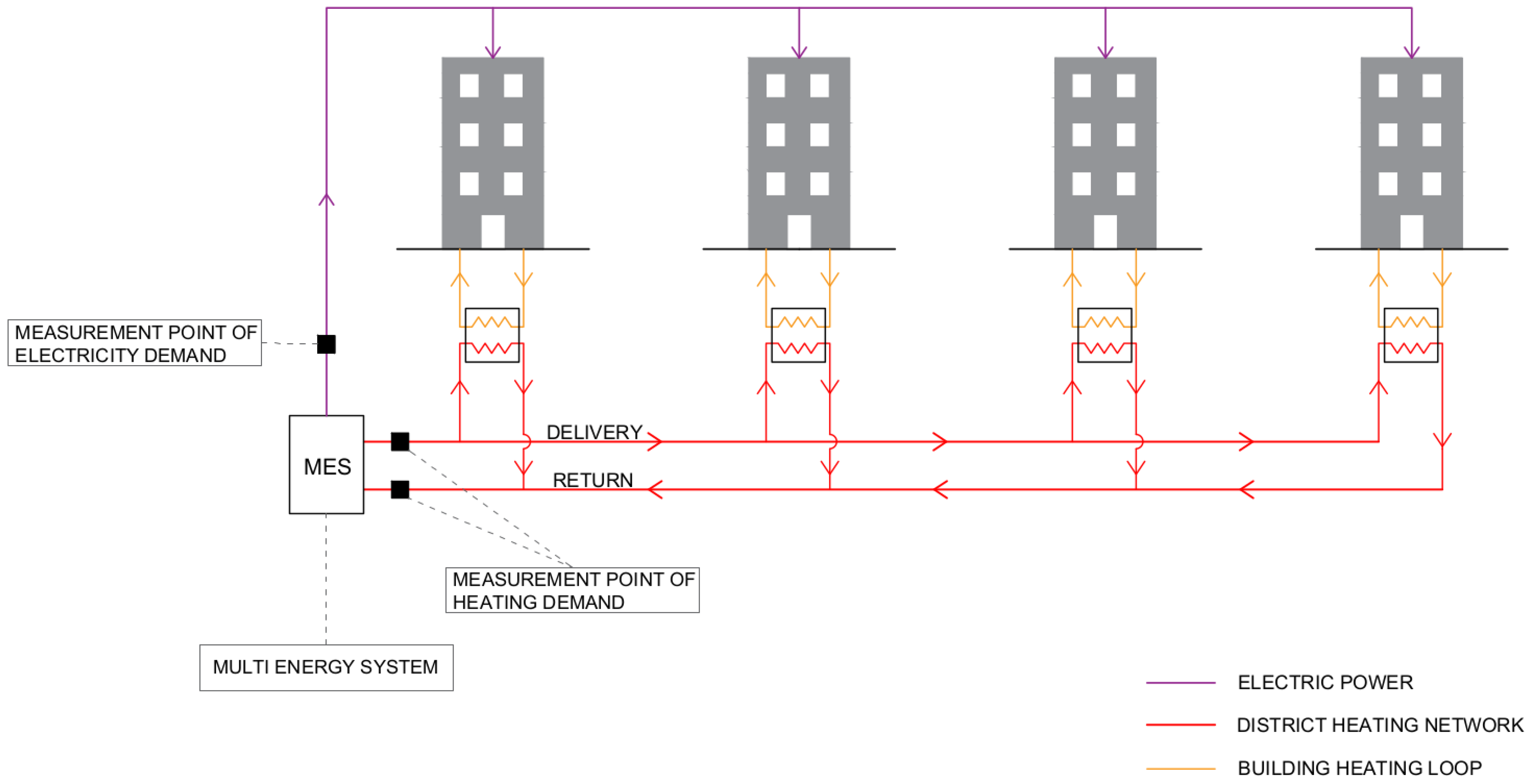
The problem addressed in this paper is of major relevance for the optimal operation of an energy system supplying heating and electricity to buildings and districts. The problem consists of predicting the daily electricity and heating consumption profiles of the district (or the single building) for the next day in order to optimize the operational schedule of the energy system. A general scheme of the investigated case studies is depicted in Figure 1.

The energy system can be either a single unit (e.g., a Combined Heat and Power engine) or a system aggregating different energy technologies (e.g., renewable sources, heat pumps, boilers, etc.), a so-called Multi-Energy System (MES). A district heating network (DHN) connects the MES with the buildings. Heating and electricity demands of the whole district are measured with an hourly or lower time resolution, and the previously measured data can be used to train the forecast method. Similarly to most real-world applications, the available pieces of information about the buildings are not sufficient to develop a thermodynamic model of the buildings (envelope heat loss coefficients, window surface, orientation, occupancy hours, number of occupants, internal air temperature) are not readily available in most practical applications). Given the available weather forecast, namely, air temperature, solar radiation, relative humidity, and wind velocity, and the past measured hourly profiles of energy consumption, there is a need for a methodology to predict the district heating and electricity demand profiles for the next day, i.e., a 24 h ahead forecast.

4. Case Studies

Although the methodology that we describe in Section 5 can be applied to a number of different energy forecasting settings, in this paper, we describe and evaluate its application to three case studies for which historical data is available, which involve both electricity and heating demands and differ in terms of consumption patterns.

The three case studies, analyzed as energy districts, are the following: a medium-size hospital located in the Emilia-Romagna Italian region, the whole Politecnico di Milano University campus, and a single building of a department belonging to the latter.

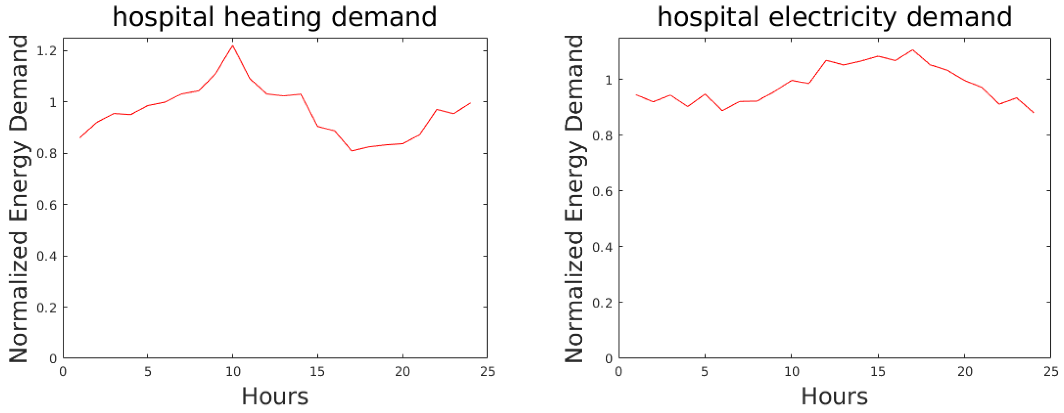
The hospital consists of several buildings with clinics, emergency rooms, and hospital rooms. Thermal power is supplied to the buildings through a district heating network. Emergency rooms and hospital rooms are heated 24/24 h a day and 7/7 days a week while clinics only during the opening hours. During the night, the temperature setpoint of the hospital rooms is slightly lowered, yielding a certain decrease in heating demand during night hours. Some rooms are equipped with air conditioning, causing an increase in electricity demand during the hot summer days. Examples of a heating demand profile during a winter day and an electricity demand profile during a summer day are reported in Figure 2.

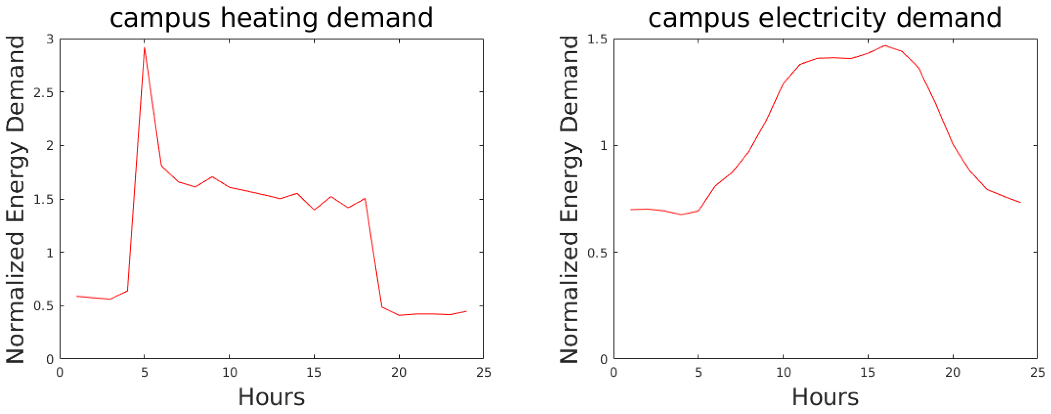
The university campus of Politecnico di Milano is located in the city center, and it consists of approximately 20 buildings interconnected by a district heating network served by boilers and CHP units. During the heating season, the thermal power provided to the buildings is adjusted so as to meet the thermal comfort setpoint during the occupancy hours (8 a.m. to 18 p.m.). Since during the night and weekends, the thermal power provided to the buildings is lowered and the internal building temperature drops below the comfort setpoint, a peak in the thermal power supply is necessary each morning at about 6–7 AM to achieve thermal comfort at 8 a.m. Compared to the profile of heating demand of the hospital case study, the university campus features a highly variable daily profile. As far as the electricity consumption is concerned, it is worth noting that it decreases during non-occupancy hours (night and weekends). Most of this non-occupancy power consumption is due to servers and lab equipment. During hot summer days, the power consumption increases because some buildings are equipped with electrically driven air conditioning systems. Examples of a heating demand profile during a winter day and an electricity demand profile during a summer day are reported in Figure 3.

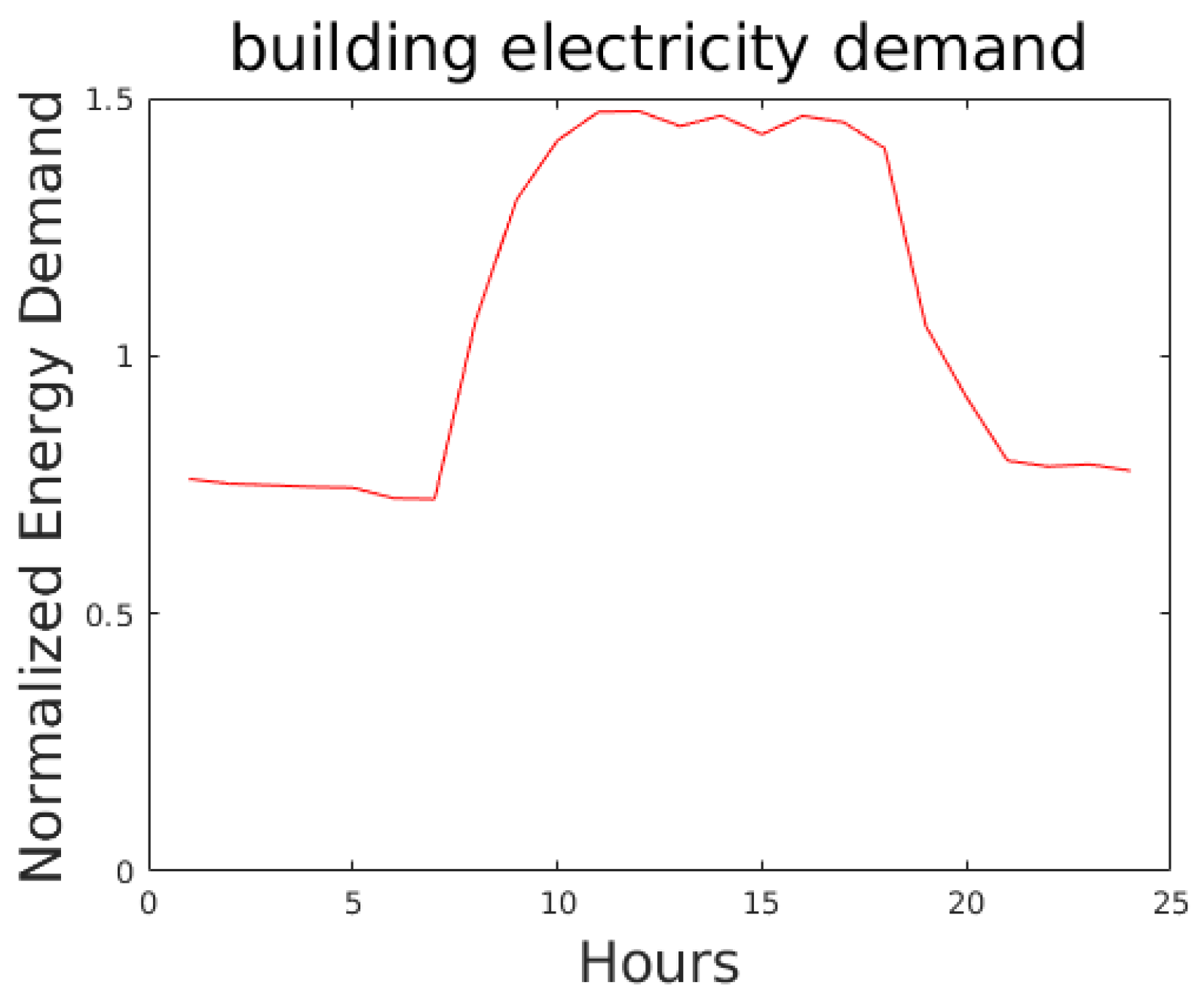
The plots of electricity demands of the single building are reported in Figure 4.

The hospital case study is first used to define and calibrate the proposed methodology, which is then successfully applied also to the two other case studies.

The predictions are obtained by training single-layer feedforward networks on the basis of a data set of historical data, including, among others, carefully selected information from the hourly energy consumption of the energy district and the hourly weather data of the region where the district is located. The considered weather data are the temperature, the solar radiation, the humidity, and the velocity of the wind. The weather data have been extracted from the website http://www.smr.arpa.emr.it/dext3r/ (accessed on 20 November 2021) for the hospital and from https://www.arpalombardia.it/ (accessed on 20 November 2021) for the whole campus and the single building.

As we shall see, the promising results obtained with our shallow ANN approach compare favourably with those provided by the autoregressive ARIMA model, SVR, and LSTM.

5. Methodology

In this section, we describe the methodology based on single-layer feedforward neural networks (SLFNs) with enriched data inputs, which we devised for the above short-term hourly energy forecasting problem. After briefly recalling some basic features of SLFNs, we first describe the important steps of input selection and data preprocessing for the considered case studies, even though they can be easily applied to other settings. Then, we present the adopted rolling horizon strategy.

5.1. Single-Layer Feedforward Neural Networks

ANNs [33,34] are well-known learning machines that have been successfully used in many application fields, such as energy, healthcare, and transportation (see, e.g., [35,36,37,38,39]). In this work, SLFNs are adopted, on the one hand, because of the compact architecture and the immediate usage, and on the other hand, because it is known that SLFNs can approximate any continuous function with arbitrary precision [40].

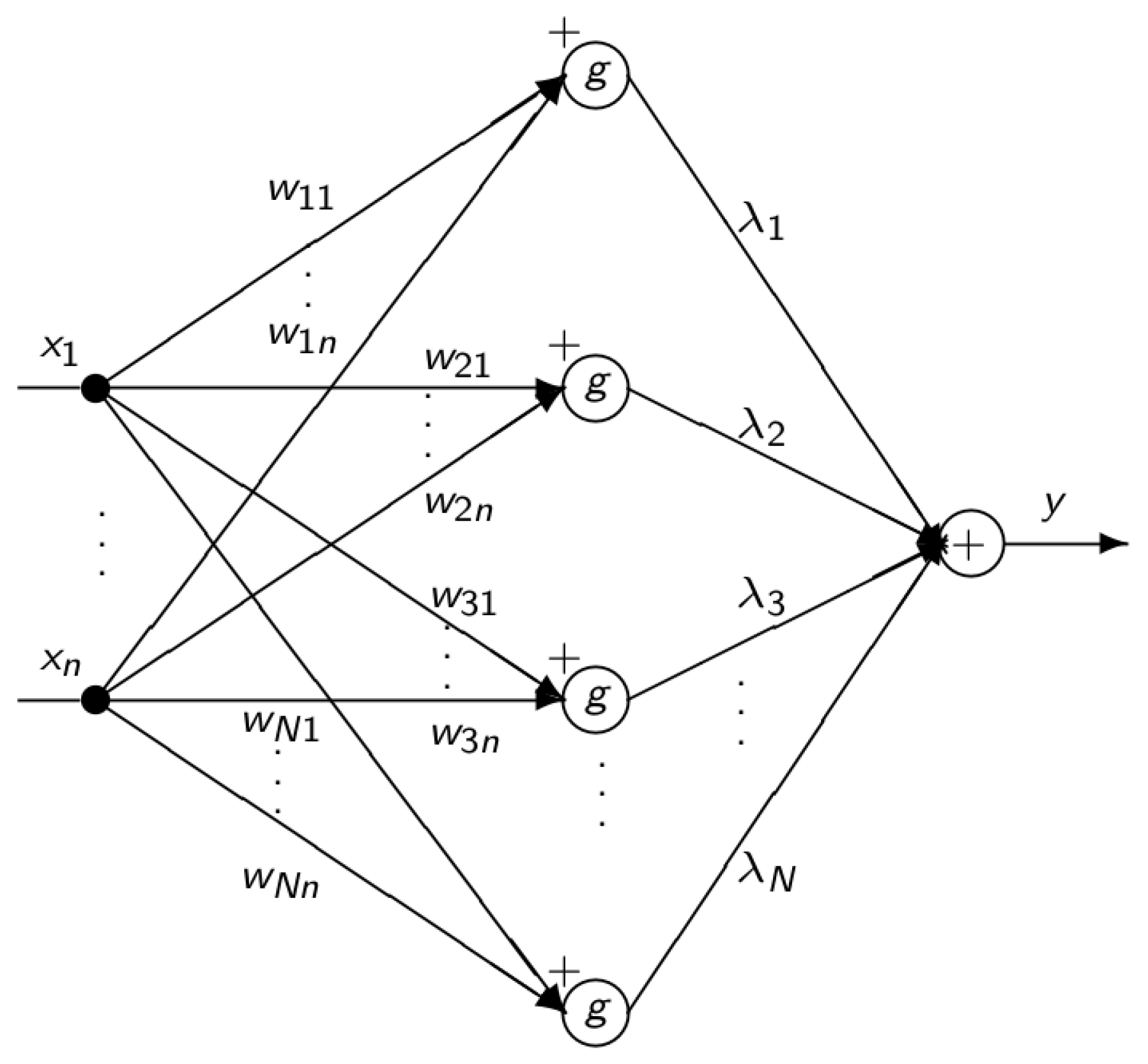
SLFNs are composed of three separated layers of interconnected processing units: an input layer with a unit for each component of the input vector of the data set, an hidden layer with an arbitrary number N of neurons, and an output layer with a single output neuron (in the case of a scalar output).

The n input components (signals) are forwarded to all the neurons of the hidden layer through weighted connections, whose weights $w_j\in {\Re }^n$ with $j=1\dots N$ are referred to as input weights. Before entering the hidden neurons, all weighted signals are summed together to generate a single entering signal. The latter is then elaborated in the hidden neuron by an arbitrary nonlinear function called the activation function and denoted as $g(·)$. The elaborated signals exiting from all the hidden neurons are forwarded to the single output unit through further weighted connections, whose weights ${\lambda }_j$, with $j=1\dots N$, are referred to as output weights. The only role of the output unit is to sum all its entering signals in order to provide the output signal denoted as $\widehat{y}$. An SLFN is depicted in Figure 5.

For a given input vector $x^p\in {\Re }^n$, the output of the SLFN ${\widehat{y}}^p\in \Re$ is computed as

$${\displaystyle {\widehat{y}}^p=\sum _{j=1}^N{\lambda }_{j}g\left(w_j^T{x}^p\right).}$$

(1)

According to the supervised learning paradigm, an SLFN is used to approximate as well as possible an unknown functional relation $y=f\left(x\right)$ by exploiting a set of historical samples in the form of input–output pairs, namely the training set ($TRS$):

$$\{(x^p,y^p),x^p\in {\Re }^n,y^p\in \Re ,p=1,\dots ,P\}.$$

(2)

During the training phase, the parameters of the SLFN are tuned by solving a challenging optimization problem that aims at reducing the overall discrepancy between the output produced by the SLFN for each input $x^p$ of $TRS$, namely ${\widehat{y}}^p$, and the desired output $y^p$.

In particular, given a $TRS$, as defined in Equation (2), the training of an SLFN consists of determining the values of the weights $w_j,{\lambda }_j,j=1,\dots ,N$, which minimize the error function

$$E(w,\lambda )=\sum _p^P\sum _{j=1}^N{({\lambda }_{j}g\left(w_j^T{x}^p\right)-y^p)}^2=\sum _p^P{({\widehat{y}}^p-y^p)}^2.$$

(3)

Minimizing Equation (3) is a very challenging task since: Equation (3) is highly nonconvex with many bad-quality local minima, flat regions, and steep-sided valleys; the computation of the gradient vector used to drive the minimization steps is carried out by a very time-consuming procedure called backpropagation; overfitting may occur, namely, the resulting model may fit “too much” of the training data and perform poorly on general unseen samples. As usual, the ability of a trained SLFN to produce accurate outputs for general inputs, referred to as generalization, is measured on a further set of samples that have not been used during the training phase, namely the testing set ($TSS$).

To overcome the above-mentioned drawbacks, in this work, we adopt the algorithm DEC proposed by Grippo et al. [12] to train SLFNs. DEC exploits an intensive decomposition strategy (in which, at each iteration, only a subset of variables are optimized while keeping the remaining ones fixed at the current value) together with a regularization technique. As shown in [12], decomposition helps to escape from poor local minima and to speedup the gradient vector computation, while the regularization tends to produce simpler models with stronger generalization performance. Hence, DEC achieves good-quality solutions in a reasonable computing time, preventing overfitting.

5.2. Selection of the Inputs and Data Preprocessing

To construct a training set suited for a supervised learning approach, the set of all collected data has been organized into samples such that each sample $p=1\dots P$ is related to a hour of a day of a week, and it consists of the input–output pair $(x^p,y^p)$ described below. The structure of the input and data preprocessing have been preliminarly investigated on the electricity and heating demand for the hospital case study and then applied to all the case studies.

In an initial phase, each pair was defined as follows.

Input $x^p$:

• Average hourly temperature (scaled in the interval $\left[0,1\right]$);
• Average hourly solar radiation (scaled in the interval $\left[0,1\right]$);
• Average hourly humidity (scaled in the interval $\left[0,1\right]$);
• Average hourly scalar wind velocity (scaled in the interval $\left[0,1\right]$);
• Day of the week (expressed as a binary 6 dimensional vector);
• Public holiday (expressed as a binary value).

Target $y^p$:

• Hourly energy demand (heating or electricity) normalized with respect to the average value of the considered time horizon.

Therefore, the input vector of each sample was initially made up of 11 components (4 for the weather, 6 for the day of the week, and 1 for the public holiday).

The choice of the four weather data was driven by a correlation analysis performed on the heating/electricity demand and weather data time series. In particular, the Pearson correlation coefficient (see, e.g., [41]) has been determined for each pair of heating/electricity demand–weather data time series together with a p-valued test to verify the null hypothesis that the two series were not correlated to each other. The null hypothesis has been rejected for every pair (with a $0.05$ significance level), showing a significant correlation between the time series. Concerning the heating, a $-0.90$ correlation coefficient has revealed a strong correlation between the heating demand and temperature, while a moderate correlation has been detected with humidity, solar radiation, and scalar wind velocity ($0.62$, $-0.30$, and $-0.30$, respectively). Concerning the electricity demand, a moderate correlation has been detected for the temperature ($0.46$), humidity ($-0.36$), and solar radiation ($0.40$), while a weak one has been detected with the scalar wind velocity ($0.09$).

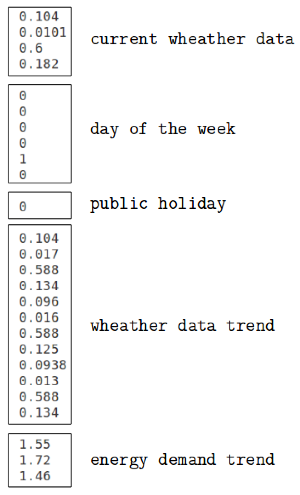
Some preliminary experiments showed that the 11 inputs were not enough to obtain a good performance since they did not take into consideration the dynamics of the system. Then, taking inspiration from the approach proposed in [42], each sample of the training set has been enriched by 15 additional inputs used to capture the trends with respect to the electricity/heating consumption and to the weather data. In particular,

• 12 additional inputs correspond to the 4 weather data in the previous 3 h;
• 3 inputs correspond to the hourly energy demand at the same hour of the same day of the week in the previous 3 weeks.

Figure 6 respresents an example of a 26-dimensional input vector incorporating the trend information.

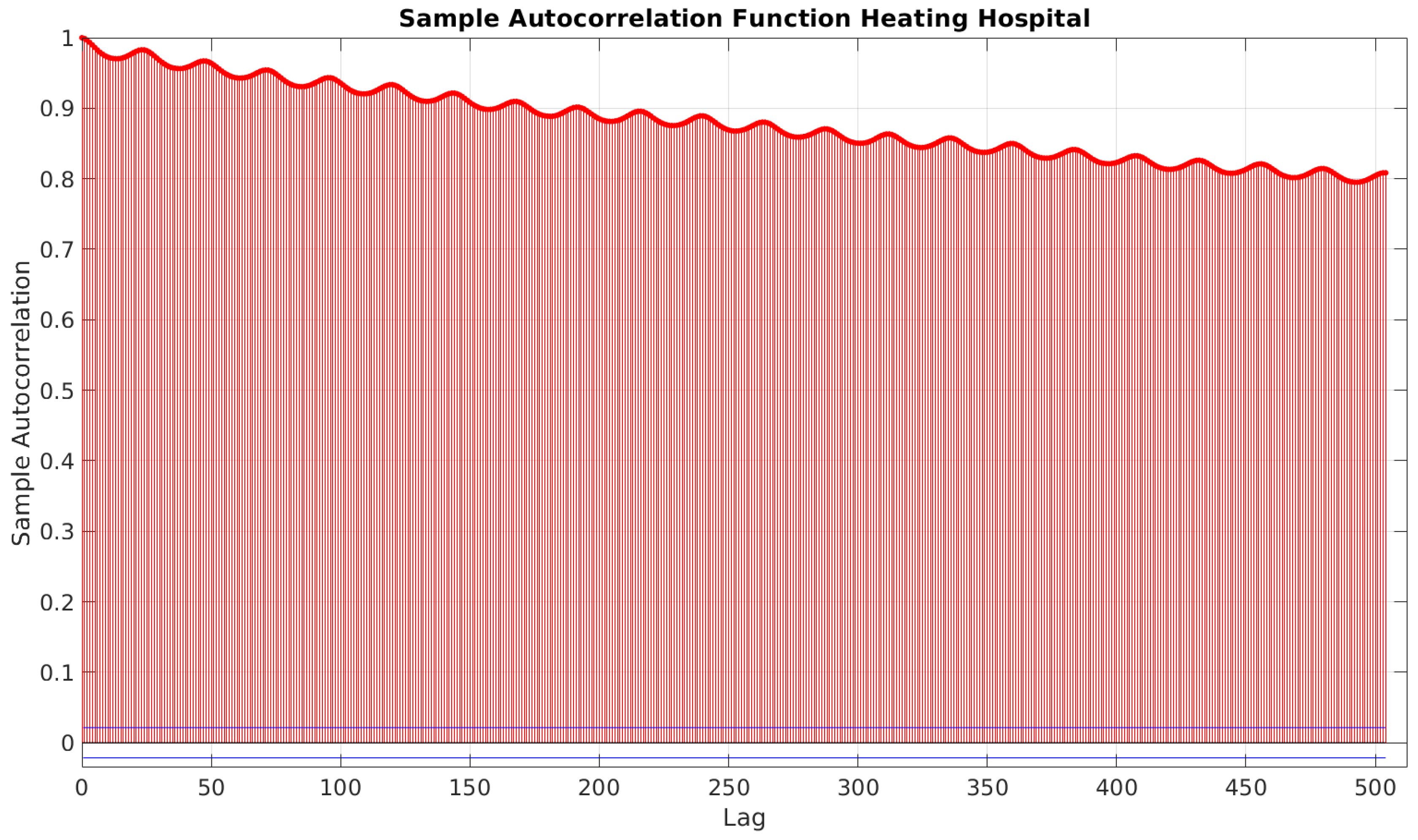
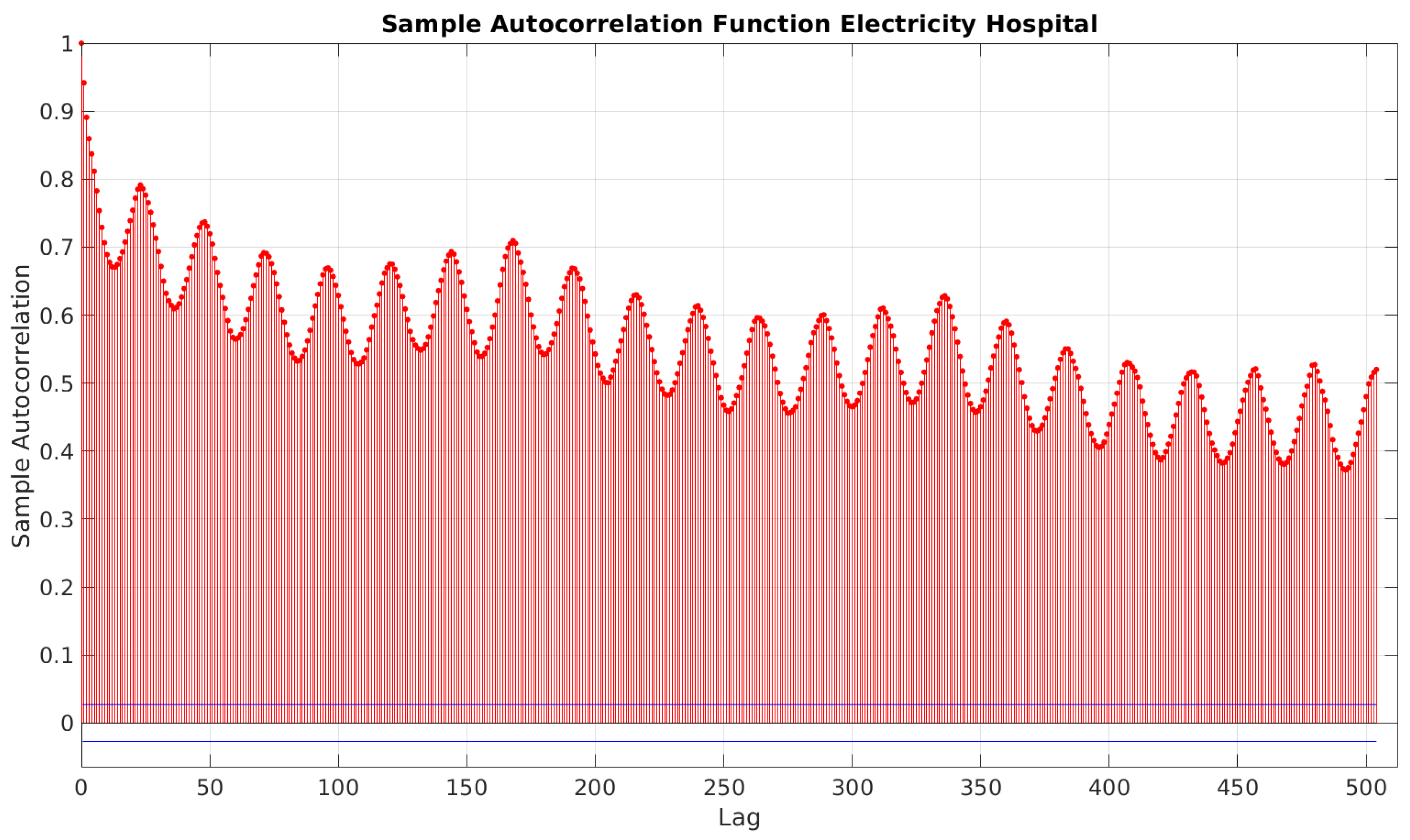
The structure of the included trend data has been driven by an autocorrelation analysis as described in [43] and implemented in the autocorr() Matlab function. By observing Figure 7, the autocorrelation plot for the electricity demand with a maximum time lag of 504 h, it is easy to notice, besides a daily pattern, a weekly pattern for which the correlation increases while approaching to the same hour of the same day of adjacents weeks, which is the time lags 168, 336, and 504 h. The three additional inputs associated to the energy demand (corresponding to the three time lags) have been included in order to provide information about this weekly pattern. Clearly, the further we move away in time, the more this weekly correlation decreases. Adding the three most recent weekly time lags allows keeping the correlation above the $0.5$ value. This choice turns out to also be appropriate for the heating demand autocorrelation (reported in Figure 8), which does not show a weekly pattern but for which a 3-week time lag maintains high autocorrelation values above $0.8$.

Concerning the additional weather inputs (for which we do not report the plots), the selection of the previous 3 h allows keeping their autocorrelation values above $0.5$ for all the weather data.

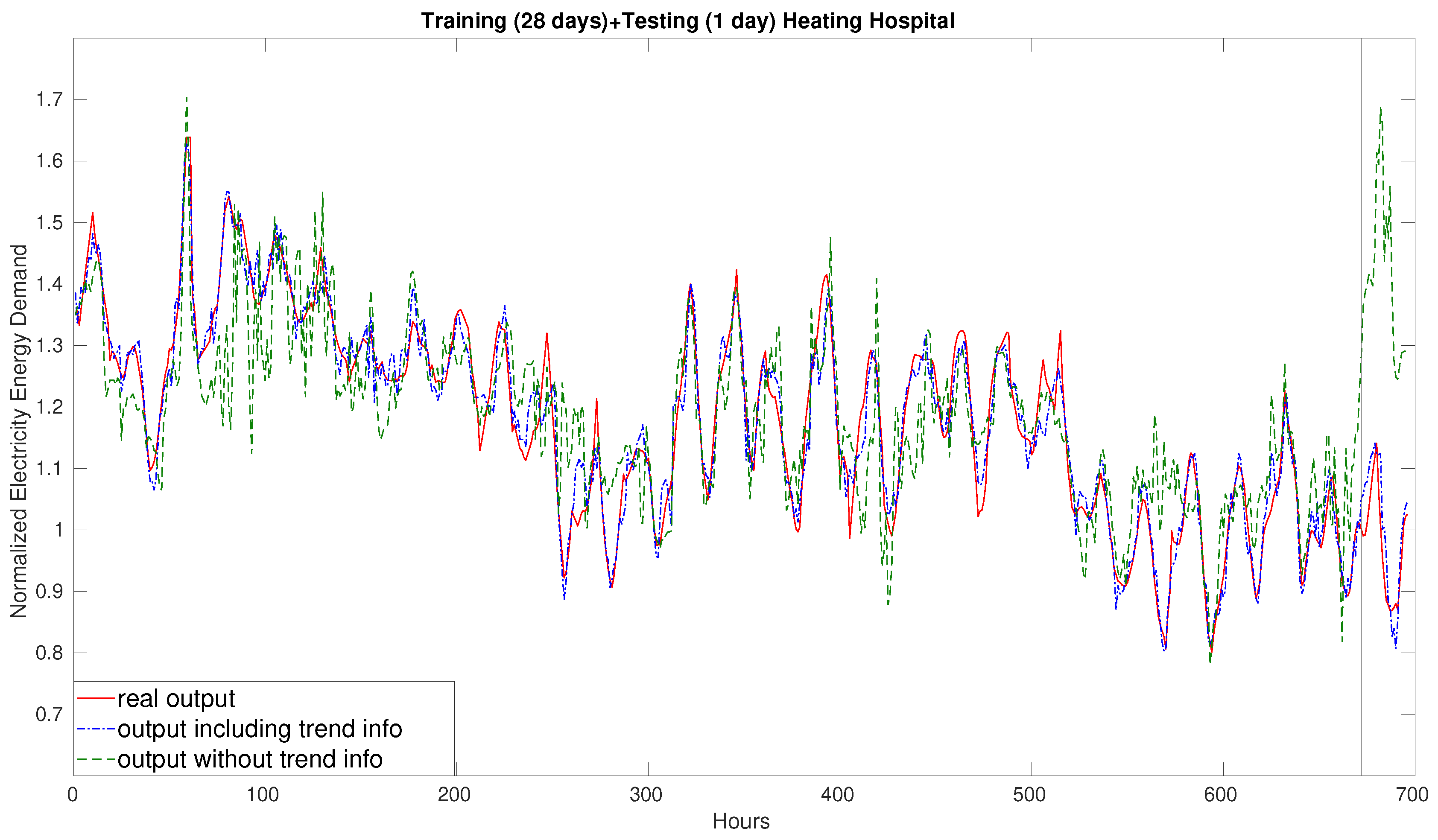
Including the trend information in the input significantly improves the performance. Figure 9 shows some preliminary training and testing experiments with and without the 15 trend inputs. In particular, the figure depicts the training and testing performance obtained by training the SLFN on a $TRS$ made up of 28 consecutive days of the hospital case study (heating demand) and then testing the trained model on the following 24 h (corresponding to the 29th day). The solid red profile is the actual output (the real hourly heating demand), the dashdot blue profile is the output generated by an SLFN trained on a data set enriched with trend data (26 inputs), while the dotted green profile is the output obtained by the SLFN without trend data (11 inputs). The profiles on the left of the vertical line correspond to the training set, while the ones on the right correspond to the testing set. It is evident that without incorporating the trend data, the SLFN has not only poor testing performance, but it is not even able to sufficiently fit the training data. On the contrary, by including the trend information in the samples, the SLFN achieves good training and testing accuracies.

It is important to note that a limited amount of data is required and that these data are easy to collect and process. Therefore, sophisticated feature learning and transfer learning techniques (see, e.g., [44,45]) are not necessary.

5.3. Rolling Horizon Strategy, Training and Testing Sets

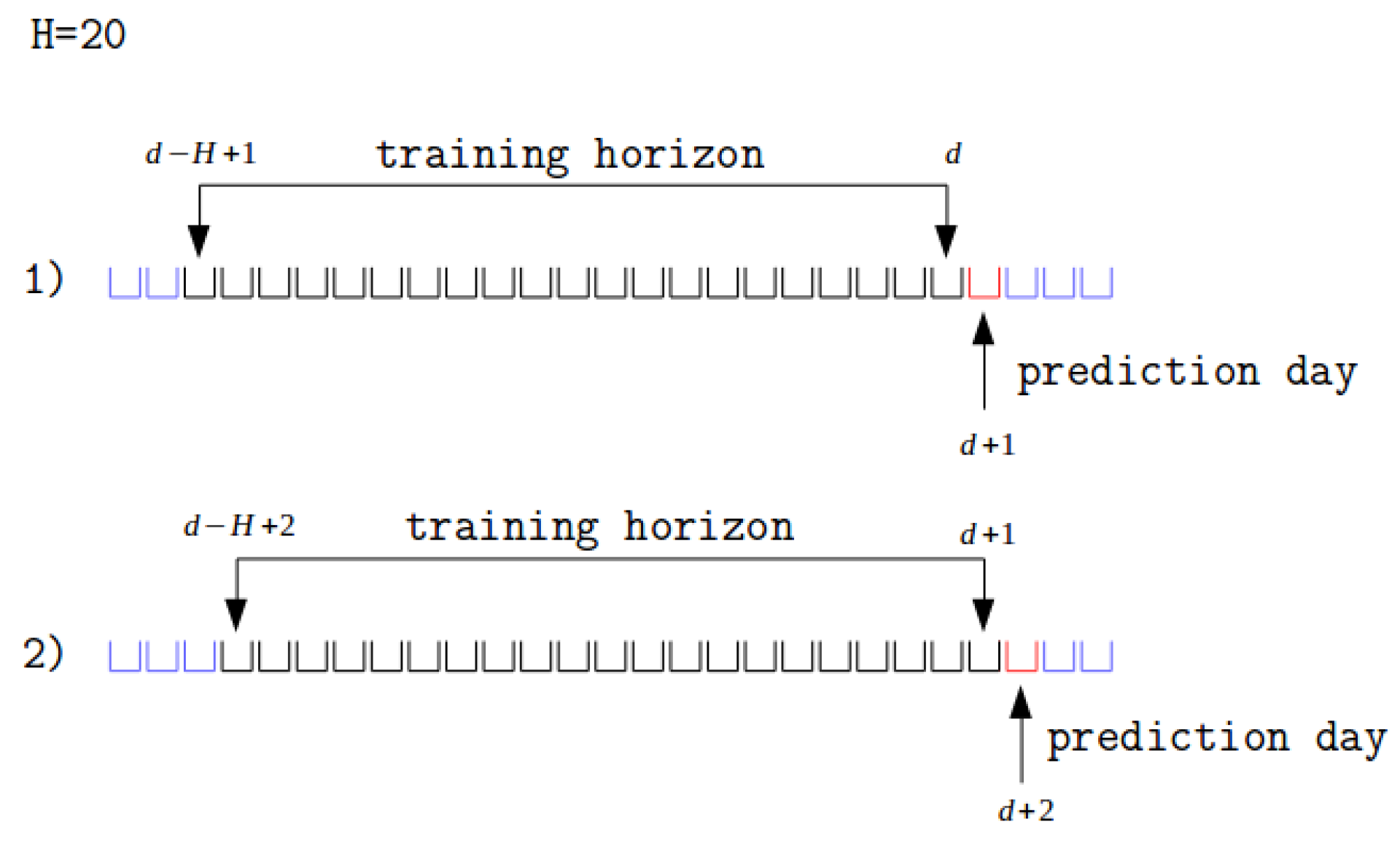
For the 24 h ahead predictive model, a rolling horizon strategy has been implemented. At the current day d, the model is trained on a $TRS$ of samples associated with the interval of days $\left[d-H+1,d\right]$, where H is the length in terms of days of the training horizon. After the training phase, the model is used to generate the prediction of the 24 hourly electricity or heating demand for the next day $d+1$. Since $TRS$ includes information of the previous H days and each sample is associated to a hour of a day, the cardinality of $TRS$ is $24·H$. Then, at day $d+1$, to predict the demand of day $d+2$, the 24 samples associated to day $d+1$ are added to $TRS$, and the least recent 24 samples of $d-H+1$ are discarded. The same procedure is iterated for the following days. See Figure 10 for a graphical example of the adopted rolling horizon strategy.

It is worth mentioning that if the rolling horizon is applied a posteriori, the input and output (weather data and energy demands) of the day of the prediction are available, and they can clearly be used, as is the case here, as $TSS$, in order to assess the performance of the proposed approach by comparing the predicted and the real output. Instead, in the case of a practical online usage of the methodology, one can construct the $TRS$ in the same way as described before because it includes past collectable data, while to generate the predictions for the next day, the only unavailable input is the weather data. However, weather data can be easily obtained from the weather forecast since the hourly average weather values can be estimated sufficiently accurately 24 h ahead.

5.4. Description of the ML Instances

Let us now describe the different instances generated from the available data to assess the performance of the proposed methodology.

It is worth pointing out that from preliminary experiments performed on the hospital case study, we observed that the best value for the training horizon H was equal to 14 days for the electricity consumption ($\left|TRS\right|=336$ samples) and 28 days for the heating one ($\left|TRS\right|=672$ samples). As shown in the sequel, these values have been successfully adopted for the other two case studies.

In order to analyze the methodology on different periods associated to different patterns of energy consumption, we divided (whenever possible) the available data of each case study into different periods, each one associated to a specific portion of the year.

We refer to $\mathcal{H}$, $\mathcal{C}$, and $\mathcal{B}$ as, respectively, the hospital, campus, and building case studies. Given a case study, say $\mathcal{H}$, the specific period is denoted as a pedex number, while the W apex indicates the heating demand, and the E apex indicates the electricity demand. For example, ${\mathcal{H}}_1^W$ indicates the first period of the heating demand for the hospital case study. A triplet “case study-period-energy demand” denotes an instance.

The instances are described in

Table 1. Description of the investigated instances. r.h. stands for the number of rolling horizon days.

Inst.	First tr.	Last tr.	First Test.	Last Test.	r.h.
${\mathcal{H}}_1^W$	4 June 2016	1 July 2016	2 July 2016	29 July 2016	28
${\mathcal{H}}_1^E$	4 June 2016	17 June 2016	18 June 2016	15 July 2016	28
${\mathcal{H}}_2^W$	29 October 2016	25 November 2016	26 November 2016	23 December 2016	28
${\mathcal{H}}_2^E$	29 October 2016	11 November 2016	12 November 2016	9 December 2016	28
${\mathcal{H}}_3^W$	22 January 2017	18 February 2017	19 February 2017	11 March 2017	21
${\mathcal{H}}_3^E$	22 January 2017	4 February 2017	5 February 2017	25 February 2017	21
${\mathcal{C}}_1^W$	6 February 2017	5 March 2017	6 March 2017	2 April 2017	28
${\mathcal{C}}_2^W$	22 January 2018	18 February 2018	19 February 2018	4 March 2018	14
${\mathcal{C}}_3^W$	31 December 2018	27 January 2019	28 January 2019	24 February 2019	28
${\mathcal{C}}_4^E$	5 March 2018	18 March 2018	19 March 2018	8 April 2018	21
${\mathcal{C}}_5^E$	4 June 2018	17 June 2018	18 June 2018	8 July 2018	21
${\mathcal{C}}_6^E$	22 October 2018	4 November 2018	5 November 2018	25 November 2018	21
${\mathcal{B}}_1^E$	5 March 2018	18 March 2018	19 March 2018	8 April 2018	21
${\mathcal{B}}_2^E$	4 June 2018	17 June 2018	18 June 2018	8 July 2018	21
${\mathcal{B}}_3^E$	22 October 2018	4 November 2018	5 November 2018	25 November 2018	21

. Each row of Table 1 is associated to a specific instance: the second and third columns report, respectively, the first and last training days of the first rolling horizon step applied to the instance, while the fourth and fifth columns correspond, respectively, to the testing days of the first and of the last rolling horizon steps. As described in Section 5.3, in the second step of the rolling horizon, all the samples of the training set associated to the first training day (column 2) are replaced by the ones associated to the first testing day (column 4), while the new testing day is the one following the previous testing day, and so on. The sixth column indicates the number of rolling horizon steps applied to the instance, corresponding to the overall number of testing days. The varying number of heating and electricity instances and of rolling horizon days depend on the availability of usable data.

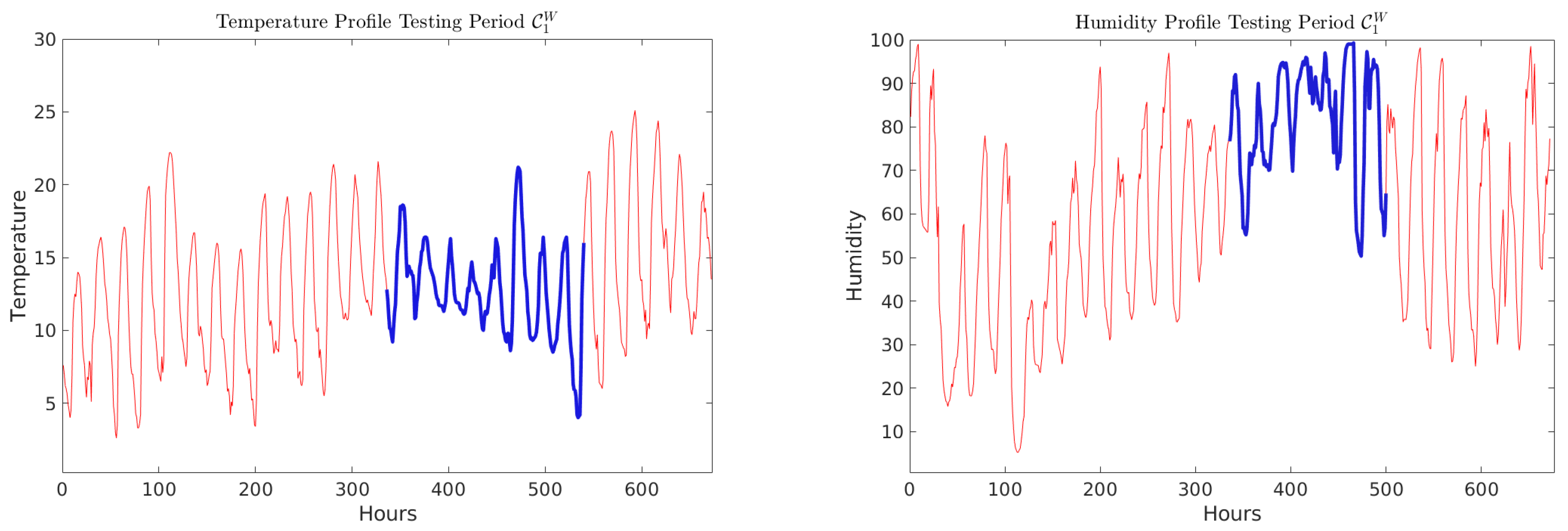
It is worth mentioning that the ${\mathcal{C}}_1^W$ instance is very challenging due to an anomalous and sudden change in weather conditions during the testing period (Figure 11 depicts the temperature and humidity profiles). This instance has been included in the experiments to test the adaptivity and the generalization of the compared methods.

6. Numerical Experiments

In this section, we present the results obtained for the considered instances by adopting an SLFN trained with the DEC algorithm, as described in Section 5.1. The results are compared with those of the autoregressive-integrated-moving-average ARIMA model, of SVR [46] (an extension of Support Vector Machine (SVMs)), and of the LSTM network.

The ARIMA techinque (see, e.g., [43]) is one of the most used methods for time series forecasting. In its general form, the ARIMA regression model is composed of a linear combination of the time series lagged observation (autoregressive part) and of a linear combination of the regression errors at various steps (moving average part). Moreover, a differencing process (consisting of replacing the time series values with the difference between consecutive values) is operated to remove periodality (integrated part). Hence, an ARIMA model is characterized by the coefficients $p,d,q$, representing, respectively, the number of terms of the autoregressive part, the number of differencing steps, and the number of terms in the moving average part. The Matlab arima function is used for the experiments.

SVMs [47] have been originally proposed for binary classification tasks and are based on determining, in the space of the input vectors, a separating surface dividing the training data into two groups according to their class membership. The separating surface is the one that maximizes its distance (margin) with respect to the closest points of the two groups. Indeed, a maximal margin surface is more likely to correctly classify unseen data points. In recent years, SVMs have been widely used in many application fields, including energy (see, e.g., [48,49,50]), and this has motivated a lot of research devoted to SVMs’ training algorithms, mainly designed for large data instances (see, e.g., [51,52,53,54]). SVMs for classification are easily extended to regression tasks, and many SVM packages also implement an SVR solver. This is the case for the SVR solver adopted in this work, which has been taken from the Matlab implementation of the well-known LIBSVM package [51].

The LSTM networks ([55]) are a kind of RNNs whose structure is designed to reduce the vanishing gradient phenomenon (see, e.g., [56]), which strongly affects the training of multi-layer neural network architectures. Differently from other deep learning methods, LSTM networks are particularly suited to model long-term temporal dependencies between variables; therefore, they are commonly used for a time series forecast in different fields, such as language modeling (see, e.g., [57]) and, as reported in Section 2, in energy consumption forecasts. The LSTM networks adopted in the experiments are taken from the Keras package of Python.

It is worth mentioning that the methods compared in the experiments cover the main approaches described in Section 2, i.e., autoregressive, machine learning, and deep learning methods.

6.1. Experimental Setting and Performance Criteria

The following SLFN architecture and hyperparameter values have been selected through a cross-validation procedure (see, e.g., [11]):

• 30 hidden neurons;
• a sigmoidal activation function $\frac{1}{1+e^{-\beta x}}$ with $\beta =1$;
• 100 internal iterations of DEC algorithm for each training set;
• a training horizon of $H=28$ days (672 hourly samples) for the heating demand and of $H=14$ days (336 hourly samples) for the electricity demand.

As highlighted in Section 5.4, the only difference between heating and electricity lies in the larger training horizon for the heating. Due to the nonconvexity of the underlying training optimization problem, the SLFN-trained models are sensitive to the random initialization of the network weights. To reduce the initialization bias, all the predictions of the SLFN are computed as the average of the predictions obtained by 10 (usually) different models corresponding to 10 different initializations of the network weights in the training phase.

For the ARIMA model, the values $p=24$, $d=1$, and $q=1$ have been chosen based on a simple enumeration procedure. Moreover, since the working days (from Monday to Friday), Saturdays, and Sundays have three different demand patterns, to improve the performance of the ARIMA model, the consumption time series have been divided into three subsequences according to the previous categories. An independent ARIMA model has been fitted for each subsequence and then used for the prediction of the corresponding days.

Concerning the SVR, the standard Gaussian kernel, which is a nonlinear mapping essentially used to obtain a nonlinear regression surface (see [11]), has been adopted. The hyperparameters of the SVR are the coefficient C, used to control overfitting, and a coefficient of the Gaussian kernel denoted as $\gamma$. By applying a cross-validation procedure, we determined the following values for the hyperparameters:

• $C=2^0$ and $\gamma =\frac{2^4}{n}$ for the heating demand;
• $C=2^8$ and $\gamma =\frac{2^{-4}}{n}$ for the electricity demand.

Furthermore, the hyperparameters of the LSTM network have been determined through cross-validation. In particular,

• 10 layers;
• the learning rate (the steplength along the gradient in the training phase) is set to $0.001$;
• 100 epochs (the number of times each sample is processed during the training).

It is worth emphasizing that for SLFN, SVR, and LSTM, the cross-validation has been applied to the hospital case study, and then the obtained hyperparameters and structure have been adopted for the experiments on the other two case studies.

The results are reported in terms of average percentage error over the period with respect to:

• the average value of demand of that period;
• the average value of each day.

In particular, let S specify a period. Let $M_S$ be the average value of the hourly electricity or heating demand over all days of period S. Given a day $d\in S$, let $M_d$ be the average value of the energy demand on day d over the 24 h. For a given hour t of a day d, let ${\widehat{y}}_{d,t}$ and $y_{d,t}$ be, respectively, the output produced by the learning machine at hour t of day d and the corresponding real consumption, and let $er{r}_{d,t}$ be the absolute value of the difference of these two values, formally

$$er{r}_{d,t}=|y_{d,t}-y_{d,t}|.$$

(4)

The percentage error at hour t at day d with respect to $M_S$ and to $M_d$ can be computed, respectively, as

$$err{S}_{d,t}=\frac{er{r}_{d,t}}{M_S}\times 100$$

(5)

and

$$err{D}_{d,t}=\frac{er{r}_{d,t}}{M_d}\times 100.$$

(6)

Now, we introduce the considered performance criteria, which are the arithmetic and geometric mean values (M and GM, respectively) of $err{S}_{d,t}$ and $err{D}_{d,t}$ over all the time horizon H:

$$\mathtt{M}\_\mathtt{errS}=\sum _{t=1}^{24}\sum _{d=1}^H\frac{err{S}_{d,t}}{24·H},$$

(7)

$$\mathtt{M}\_\mathtt{errD}=\sum _{t=1}^{24}\sum _{d=1}^H\frac{err{D}_{d,t}}{24·H},$$

(8)

$$\mathtt{GM}\_\mathtt{errS}=\sqrt[24·H]{\prod _{t=1}^{24}\prod _{d=1}^{H}err{S}_{d,t}},$$

(9)

$$\mathtt{GM}\_\mathtt{errD}=\sqrt[24·H]{\prod _{t=1}^{24}\prod _{d=1}^{H}err{D}_{d,t}}.$$

(10)

The difference between $\mathtt{M}\_\mathtt{errS}$ and $\mathtt{M}\_\mathtt{errD}$ is that $\mathtt{M}\_\mathtt{errD}$ tends to unfairly penalize small errors for low-level demand days (weekends), while $\mathtt{M}\_\mathtt{errS}$ is an error measure weighted with respect to the average demand of the period, so it is not affected by the weekends demand reduction; however, it provides less information about more “local” aspects. Therefore, the difference between the two error measures is more remarkable in case studies with a high energy demand difference among working days and weekends (campus).

The geometric mean, which is less sensitive to the different scales among averaged values than the arithmetic one, has been reported since different levels of demands in different hours/days may cause nonuniform error ranges.

6.2. Results

Table 2. Results obtaiined for the heating energy demand.

	$\mathtt{M}\_\mathtt{errS}$	$\mathtt{GM}\_\mathtt{errS}$	$\mathtt{M}\_\mathtt{errD}$	$\mathtt{GM}\_\mathtt{errD}$
${\mathcal{H}}_1^W$
SLFN	$5.22\%$	$3.39\%$	$4.89\%$	$3.21\%$
SVR	$9.50\%$	$7.15\%$	$9.27\%$	$6.76\%$
ARIMA	$7.20\%$	$4.36\%$	$7.72\%$	$4.75\%$
LSTM	5.99%	$3.73\%$	$6.60\%$	$4.06\%$
${\mathcal{H}}_2^W$
SLFN	$5.74\%$	$3.84\%$	$4.55\%$	$3.14\%$
SVR	$13.16\%$	$9.92\%$	$10.40\%$	$8.11\%$
ARIMA	$9.39\%$	$6.15\%$	$8.70\%$	$5.82\%$
LSTM	25.21%	$16.92\%$	$19.64\%$	$13.83\%$
${\mathcal{H}}_3^W$
SLFN	$5.58\%$	$2.80\%$	$6.69\%$	$3.13\%$
SVR	$7.12\%$	$4.29\%$	$8.44\%$	$4.78\%$
ARIMA	$7.82\%$	$3.48\%$	$9.52\%$	$3.88\%$
LSTM	12.28%	$7.65\%$	$11.95\%$	$7.23\%$
${\mathcal{C}}_1^W$
SLFN	$11.74\%$	$6.86\%$	$26.37\%$	$14.41\%$
SVR	$13.52\%$	$8.39\%$	$33.07\%$	$17.62\%$
ARIMA	$20.56\%$	$11.49\%$	$42.74\%$	$24.14\%$
LSTM	28.29%	$19.42\%$	$69.78\%$	$40.79\%$
${\mathcal{C}}_2^W$
SLFN	$11.88\%$	$6.46\%$	$8.97\%$	$5.20\%$
SVR	$14.14\%$	$8.34\%$	$10.55\%$	$6.71\%$
ARIMA	$13.36\%$	$7.32\%$	$14.94\%$	$8.02\%$
LSTM	25.66%	$15.72\%$	$20.75\%$	$12.65\%$
${\mathcal{C}}_3^W$
SLFN	$12.63\%$	$7.21\%$	$15.42\%$	$7.90\%$
SVR	$13.81\%$	$7.94\%$	$17.58\%$	$8.70\%$
ARIMA	$23.73\%$	$12.70\%$	$19.16\%$	$10.22\%$
LSTM	20.94%	$12.88\%$	$25.46\%$	$14.11\%$

and

Table 3. Results obtained for the electricity energy demand.

	$\mathtt{M}\_\mathtt{errS}$	$\mathtt{GM}\_\mathtt{errS}$	$\mathtt{M}\_\mathtt{errD}$	$\mathtt{GM}\_\mathtt{errD}$
${\mathcal{H}}_1^E$
SLFN	$8.35\%$	$3.62\%$	$6.63\%$	$3.15\%$
SVR	$11.56\%$	not available	$9.66\%$	not available
ARIMA	$9.98\%$	$4.73\%$	$10.18\%$	$4.86\%$
LSTM	9.40%	$4.28\%$	$12.51\%$	$5.89\%$
${\mathcal{H}}_2^E$
SLFN	$4.53\%$	$2.40\%$	$4.60\%$	$2.47\%$
SVR	$6.48\%$	$4.00\%$	$6.69\%$	$4.11\%$
ARIMA	$8.70\%$	$3.94\%$	$9.67\%$	$4.12\%$
LSTM	7.35%	$4.70\%$	$7.59\%$	$4.83\%$
${\mathcal{H}}_3^E$
SLFN	$4.39\%$	$2.42\%$	$4.54\%$	$2.54\%$
SVR	$5.49\%$	$3.50\%$	$5.70\%$	$3.68\%$
ARIMA	$13.90\%$	$7.16\%$	$11.82\%$	$6.24\%$
LSTM	7.10%	$4.53\%$	$7.40\%$	$4.76\%$
${\mathcal{C}}_1^E$
SLFN	$6.29\%$	$3.04\%$	$7.12\%$	$3.29\%$
SVR	$7.37\%$	$3.83\%$	$8.19\%$	$4.15\%$
ARIMA	$8.19\%$	$4.09\%$	$9.41\%$	$4.43\%$
LSTM	9.47%	$4.89\%$	$9.70\%$	$5.30\%$
${\mathcal{C}}_2^E$
SLFN	$5.05\%$	$3.12$	$4.82\%$	$2.95\%$
SVR	$5.36\%$	$3.42\%$	$5.23\%$	$3.24\%$
ARIMA	$4.94\%$	$2.98\%$	$4.79\%$	$2.82\%$
LSTM	13.38%	$7.15\%$	$12.26\%$	$6.77\%$
${\mathcal{C}}_3^E$
SLFN	$5.83\%$	$2.87\%$	$5.44\%$	$2.70\%$
SVR	$8.96\%$	$6.78\%$	$8.35\%$	$5.72\%$
ARIMA	$5.51\%$	$3.03\%$	$5.16\%$	$2.85\%$
LSTM	21.13%	$10.06\%$	$18.73\%$	$9.47\%$
${\mathcal{B}}_1^E$
SLFN	$5.32\%$	$2.66\%$	$5.72\%$	$2.76\%$
SVR	$7.10\%$	$4.02\%$	$7.73\%$	$4.17\%$
ARIMA	$7.30\%$	$3.79\%$	$7.86\%$	$3.93\%$
LSTM	9.84%	$5.29\%$	$10.06\%$	$5.48\%$
${\mathcal{B}}_2^E$
SLFN	$4.11\%$	$2.58$	$3.97\%$	$2.54\%$
SVR	$4.95\%$	$3.40\%$	$4.83\%$	$3.35\%$
ARIMA	$3.70\%$	$2.51\%$	$3.62\%$	$2.46\%$
LSTM	10.28%	$5.17\%$	$9.84\%$	$5.09\%$
${\mathcal{B}}_3^E$
SLFN	$5.96\%$	$3.31\%$	$5.63\%$	$3.14\%$
SVR	$7.21\%$	not available	$6.63\%$	not available
ARIMA	6.07%	$3.48\%$	$5.90\%$	$3.30\%$
LSTM	17.68%	$8.76\%$	$16.00\%$	$8.31\%$

report the four performance values obtained by the SLFN, SVR, ARIMA, and LSTM methods on the considered instances for, respectively, the heating and electricity energy demands.

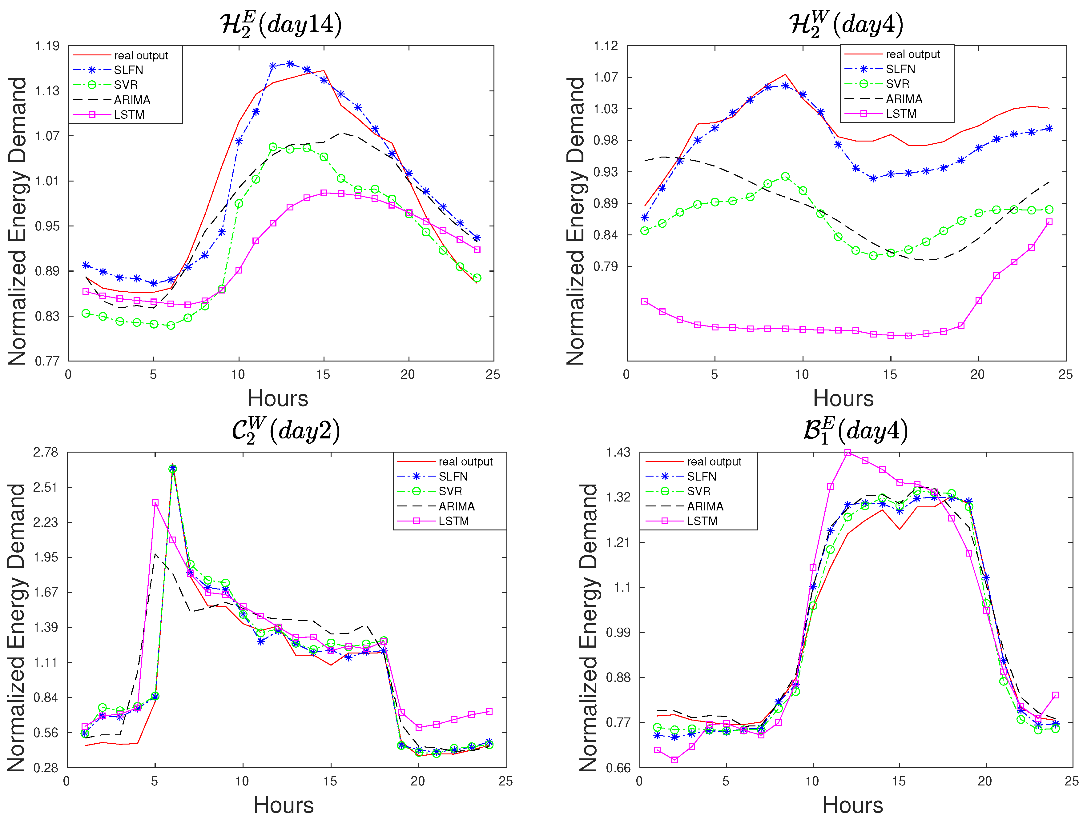
The tables show that the better performances (highlighted in bold) are achieved by SLFN on 12 instances out of 15 for all the scores. On ${\mathcal{B}}_2^E$ and ${\mathcal{C}}_2^E$, the ARIMA method is slightly better, even if the performance difference with respect to SLFN is less than $1\%$ on all scores. Notice that on those instances in which SLFN results are favorable, the performance difference is often more marked (see, e.g., ${\mathcal{H}}_3^W$). On ${\mathcal{C}}_3^E$, SLFN is better in terms of geometric mean while ARIMA in terms of arithmetic mean.

Concerning the $\mathtt{M}\_\mathtt{errS}$ score, for SLFN, it is always below $13\%$ (often below $6\%$). SVR, ARIMA, and LSTM have a maximum $\mathtt{M}\_\mathtt{errS}$ score of $14.14\%$, $23.73\%$, and $28.29\%$, respectively.

Concerning the $\mathtt{M}\_\mathtt{errD}$ score, SLFN has a maximum value of $26.37\%$ (often below $6\%$), while SVR, ARIMA, and LSTM have one of $33.07\%$, $42.74\%$, and $69.78\%$, respectively.

In the campus case study, featuring a great energy demand difference among working days and weekends, the difference between $\mathtt{M}\_\mathtt{errS}$ and $\mathtt{M}\_\mathtt{errD}$ tends to be more marked.

Concerning $\mathtt{GM}\_\mathtt{errS}$ and $\mathtt{GM}\_\mathtt{errD}$, the results are analogous.

It is worth pointing out that on the challenging instance ${\mathcal{C}}_1^W$ mentioned in Section 5.4, SLFN performs significantly better than the other methods.

Surprisingly, in our instances, the performance of LSTM appears to be less competitive. This may be due to the relatively short training horizons, which may be more suited for simpler models.

Finally, Figure 12 reports typical profiles of the 24 h daily predictions generated by the three methods in some rolling horizon steps on different instances.

7. Concluding Remarks

Overall, the results obtained for the three considered case studies indicate that carefully selected inputs often allow the shallow neural network approach and Support Vector Regression to achieve error scores significantly smaller than $10\%$.

Single-layer feedforward networks with enriched data inputs and the efficient decomposition-based training algorithm DEC turn out to be more promising and robust on the considered set of instances. It is worth emphasizing that only a few hyperparameters need to be tuned and that the simple network architecture with 30 hidden units, calibrated for the first case study, has then been successfully used for the two other case studies.

The good performance obtained in predicting both heating and electricity demands on different types of energy districts (hospital, university campus, and single building) confirm the flexibility and generalization ability of the proposed approach. Because of its simplicity, flexibility, and forecast accuracy, it may be useful for operators of Multi-Energy Systems (e.g., energy service companies) and microgrids, which need to manage several systems with limited knowledge of the users’ habits, district heating network features, and buildings.

Future work includes, on the one hand, the application of the approach to other case studies and, on the other hand, the development of systematic ways to perform the data analysis at the basis of the careful input selection process.