

Sector Coupling Potential of a District Heating Network by Consideration of Residual Load and CO2 Emissions


Abstract
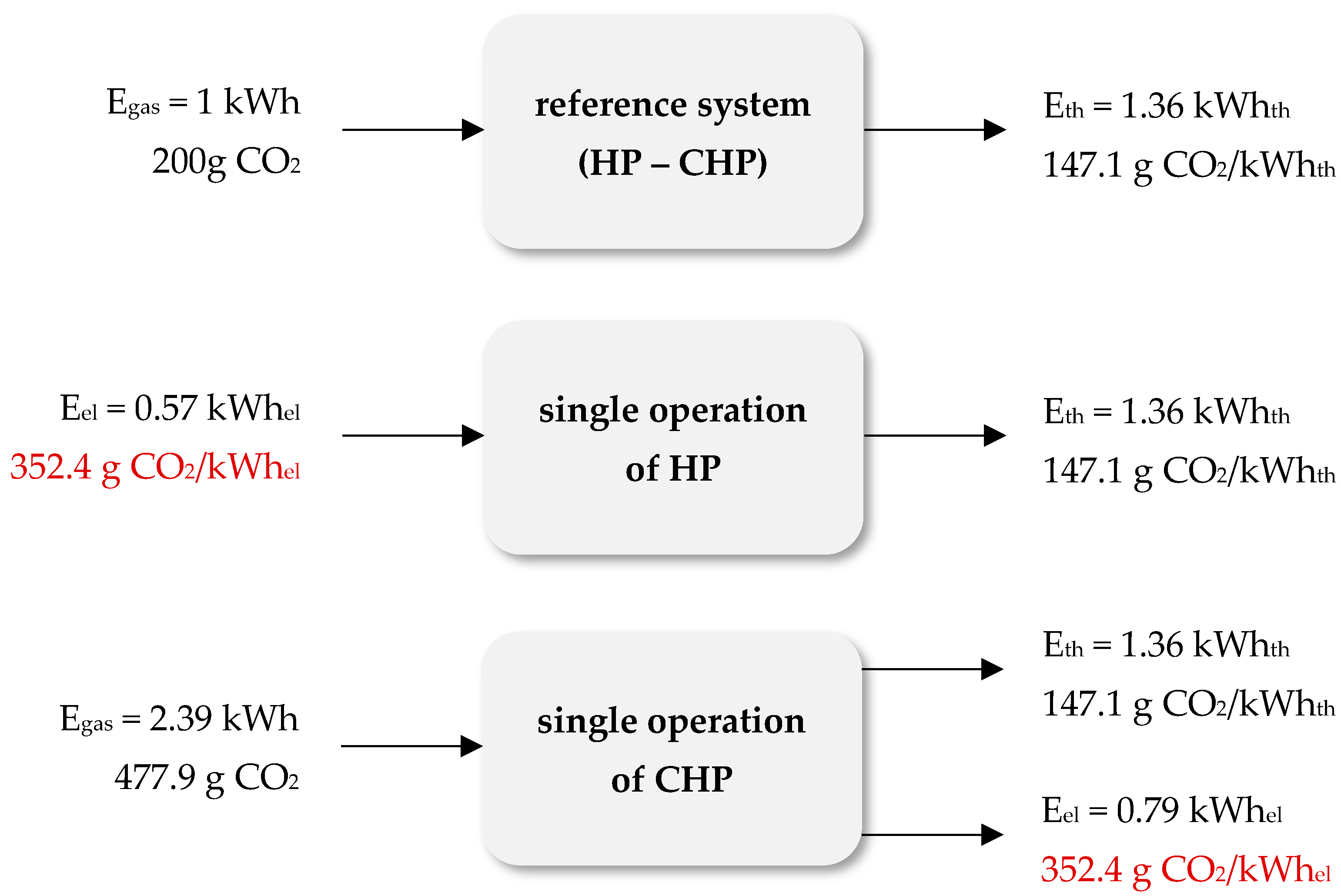
:
1. Motivation and Objectives
2. Residual Loads and CO2 Emissions of the German Power Grid
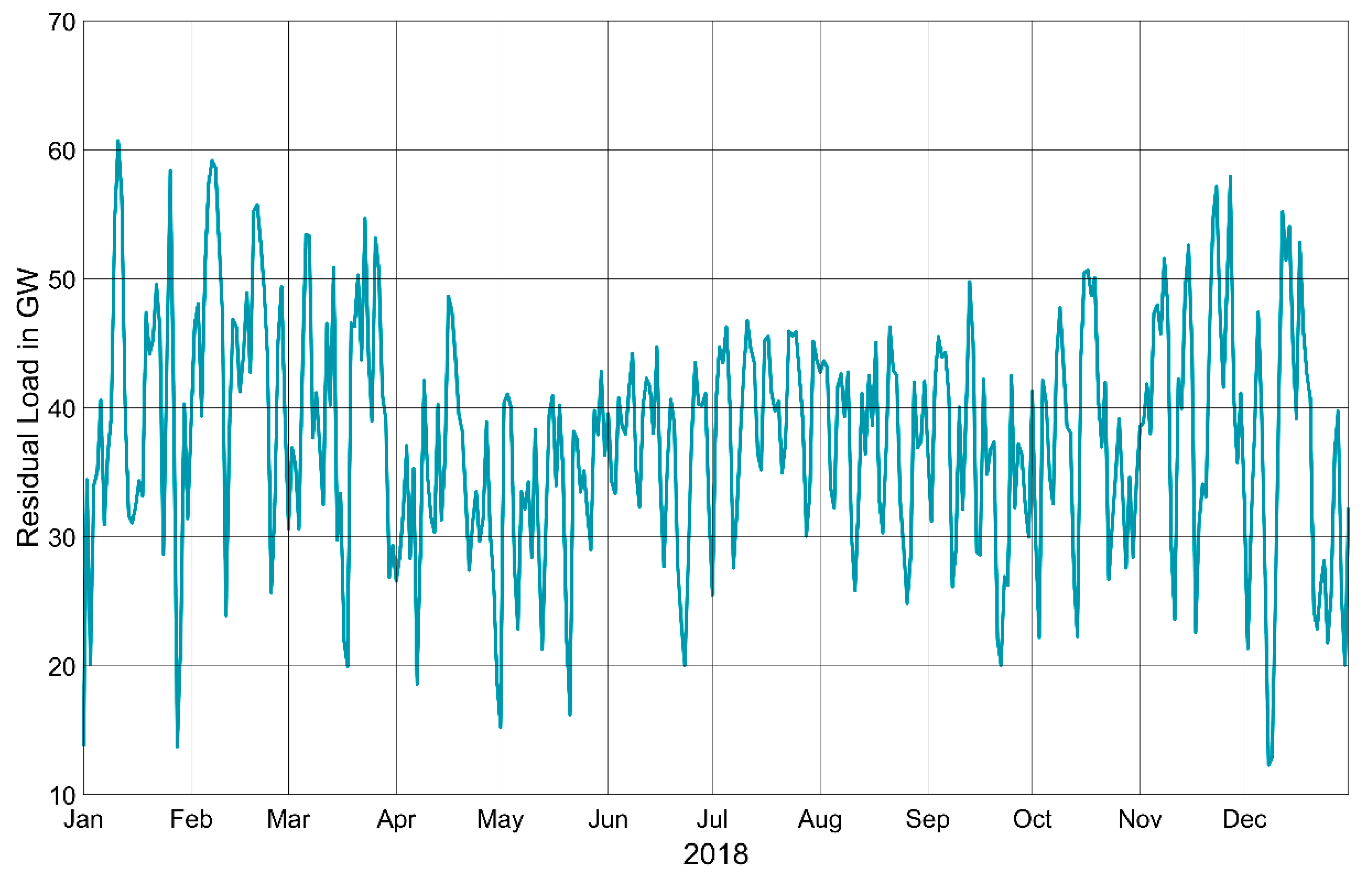
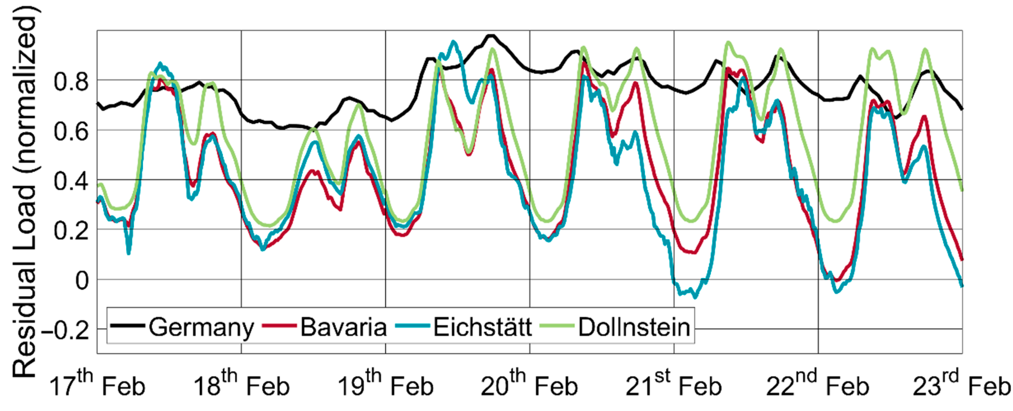
2.1. Residual Load
- hydropower,
- photovoltaics,
- wind onshore,
- wind-offshore and
- other RE (geothermal, landfill, sewage, and mine gas).
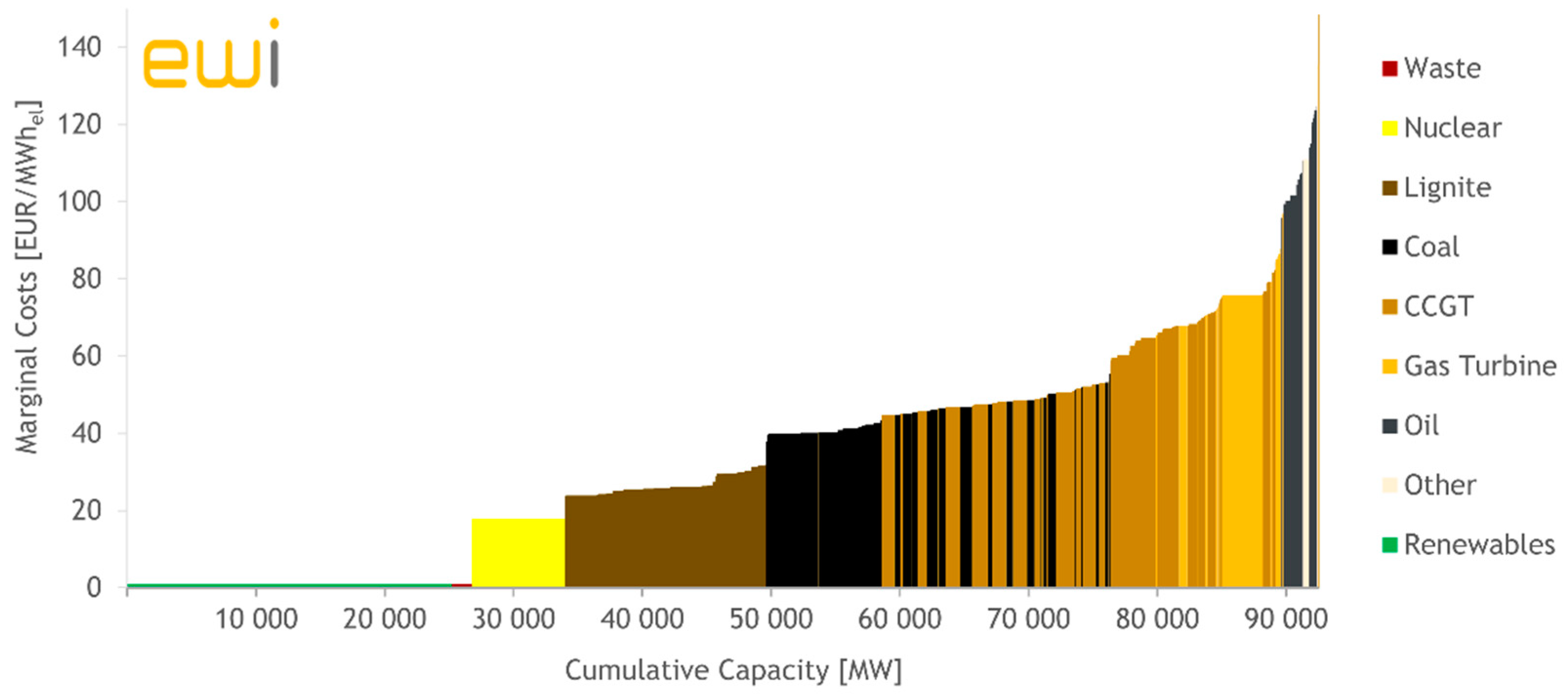
2.2. CO2 Emissions
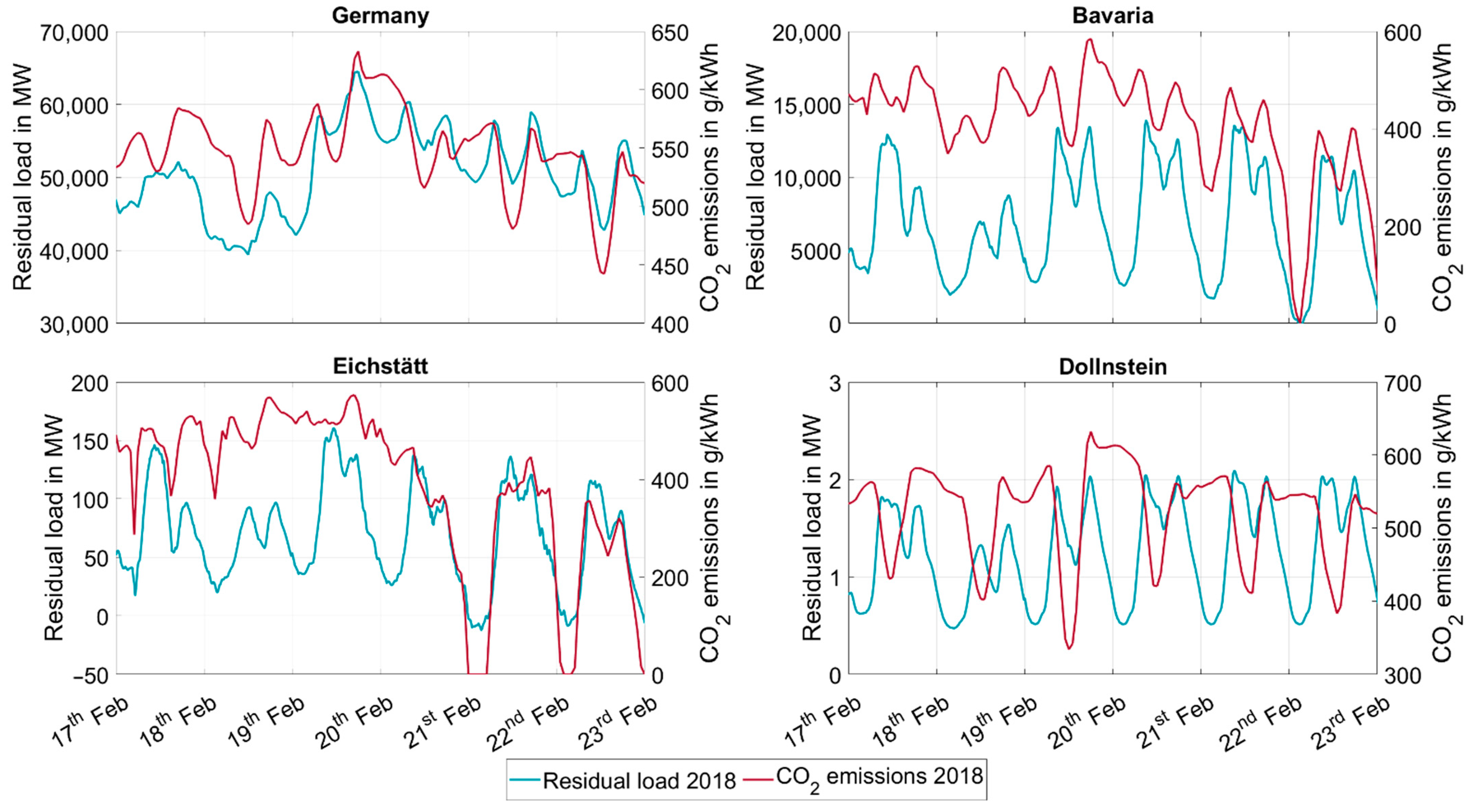
2.3. Correlation between Residual Load and CO2 Emissions
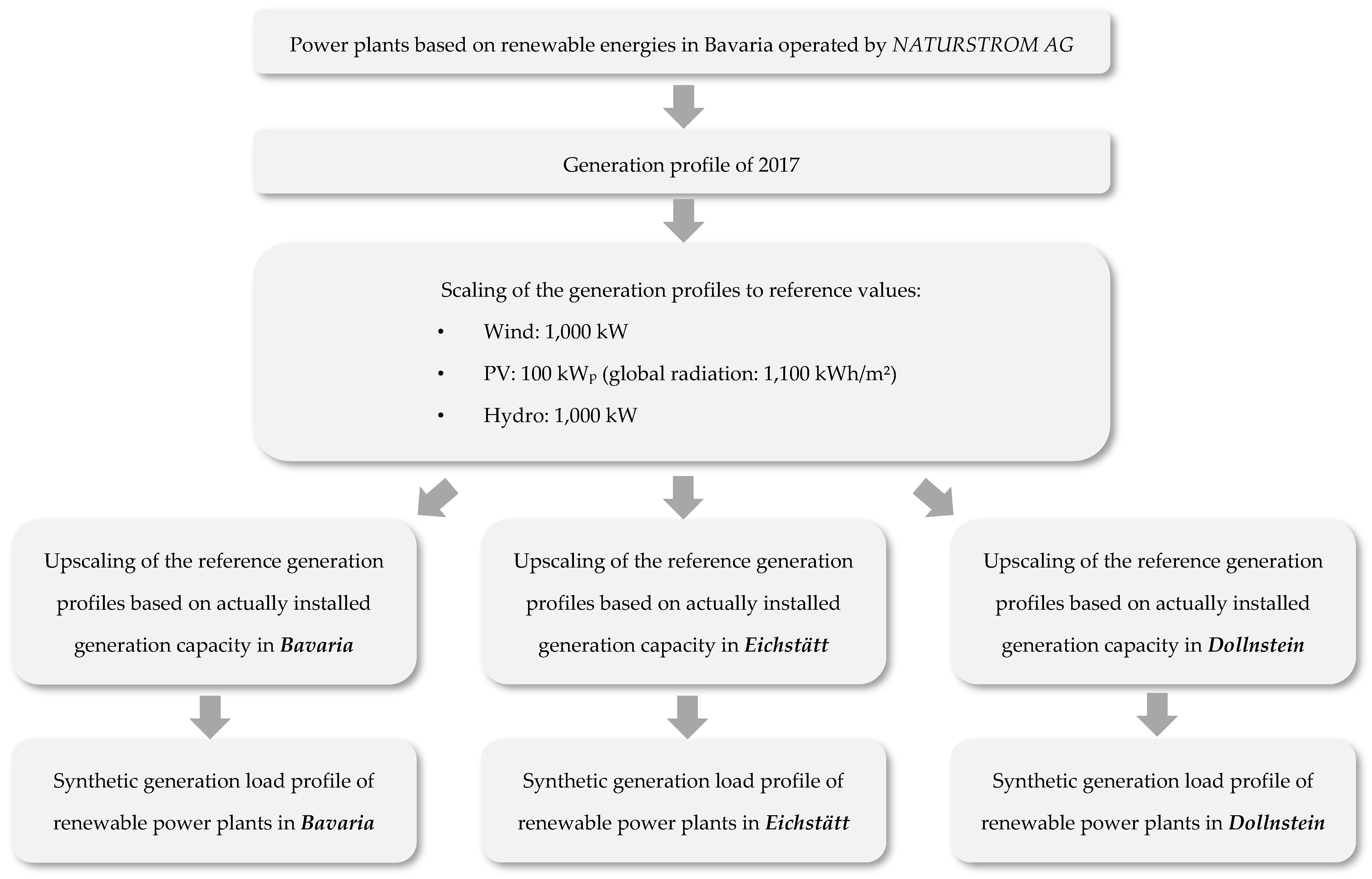
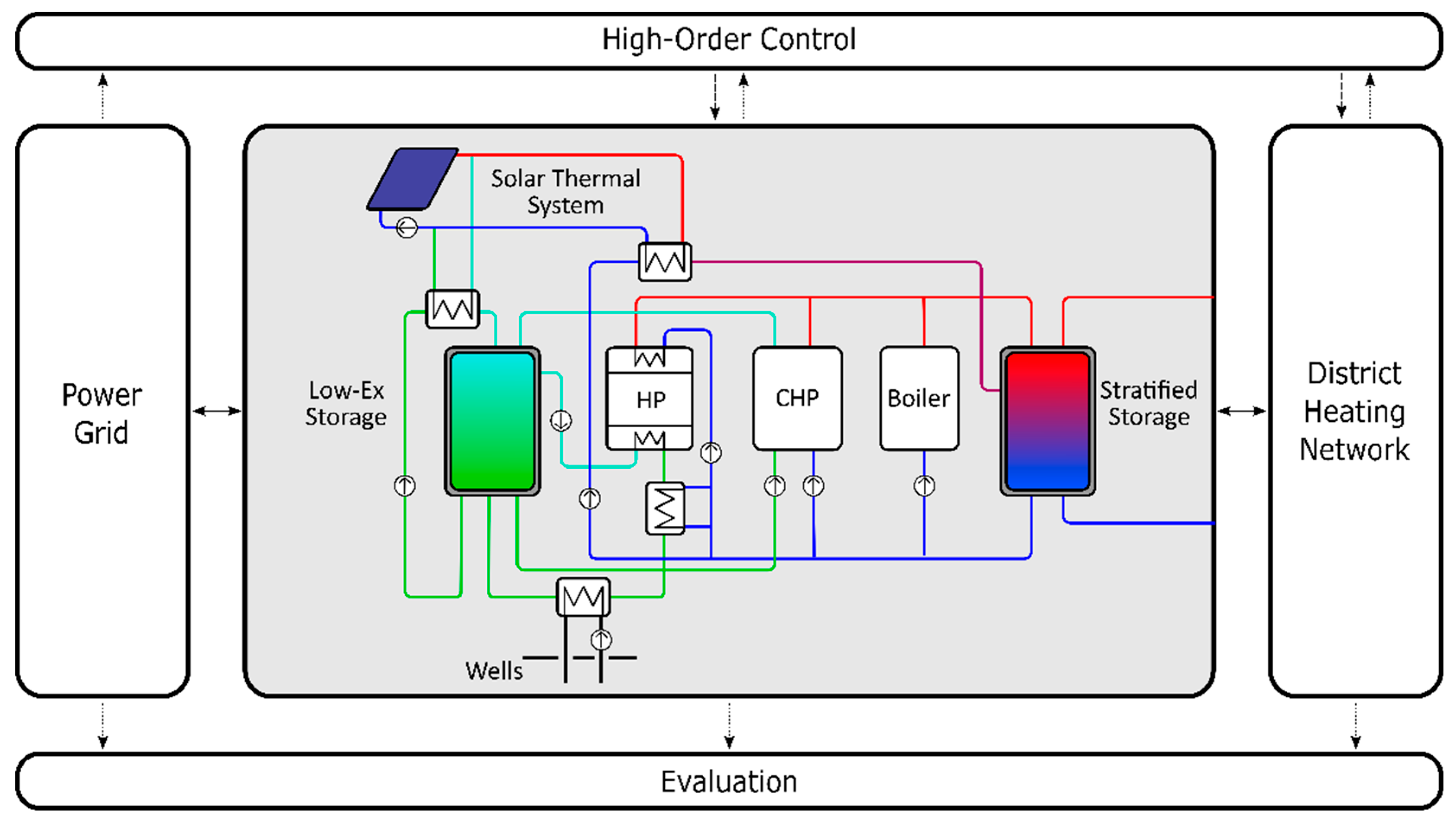
3. The DHN of Dollnstein and Its Modelling
4. Sector Coupling in the Simulation Model
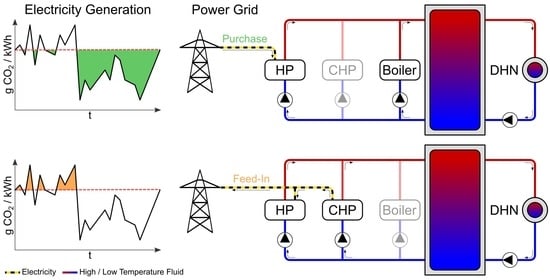
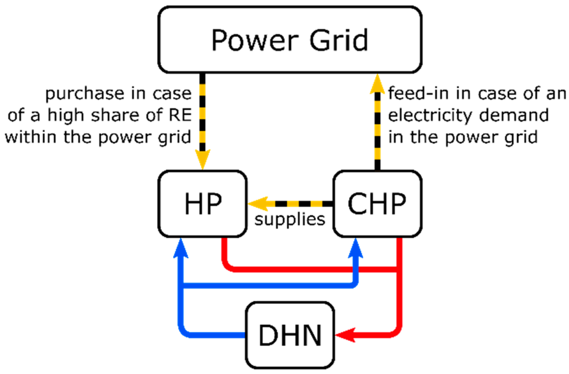
4.1. Control by Residual Load
4.2. Control by CO2 Emissions
4.3. Data Availability for Control Strategies
5. Results and Discussion
5.1. Operating under Consideration of Residual Load
5.2. Operating under Consideration of CO2 Emissions
6. Conclusions
Author Contributions
Funding
Institutional Review Board Statement
Informed Consent Statement
Data Availability Statement
Conflicts of Interest
References
- Eurostat. Electricity and Heat Statistics. Available online: https://ec.europa.eu/eurostat/statistics-explained/index.php?title=Electricity_and_heat_statistics#Installed_electrical_capacity (accessed on 28 January 2022).
- Eurostat. Electricity Production, Consumption and Market Overview. Available online: https://ec.europa.eu/eurostat/statistics-explained/index.php?title=Electricity_production,_consumption_and_market_overview#Electricity_generation (accessed on 28 January 2022).
- Umweltbundesamt. Erneuerbare Energien in Deutschland; Umweltbundesamt: Dessau-Roßlau, Germany, 2021. [Google Scholar]
- Deutsche Energie-Agentur GmbH. Dena-Gebäudereport 2021—Fokusthemen zum Klimaschutz im Gebäudebereich; Deutsche Energie-Agentur GmbH: Berlin, Germany, 2021. [Google Scholar]
- Lund, H.; Mathiesen, B.V.; Connolly, D.; Østergaard, P.A. Renewable Energy Systems—A Smart Energy Systems Approach to the Choice and Modelling of 100 % Renewable Solutions. Chem. Eng. Trans. 2014, 39, 1–6. [Google Scholar] [CrossRef]
- Lund, H.; Østergaard, P.A.; Connolly, D.; Mathiesen, B.V. Smart energy and smart energy systems. Energy 2017, 137, 556–565. [Google Scholar] [CrossRef]
- Ahn, H.; Miller, W.; Sheaffer, P.; Tutterow, V.; Rapp, V. Opportunities for installed combined heat and power (CHP) to increase grid flexibility in the U.S. Energy Policy 2021, 157, 112485. [Google Scholar] [CrossRef]
- Epik, O.; Zubenko, V. Usage of biomass CHP for balancing of power grid in Ukraine. In E3S Web of Conference; EDP Sciences: Les Ulis, France, 2019; Volume 112. [Google Scholar] [CrossRef]
- Rinne, S.; Syri, S. The possibilities of combined heat and power production balancing large amounts of wind power in Finland. Energy 2015, 82, 1034–1046. [Google Scholar] [CrossRef]
- Ishikawa, S.; Connell, N.O.; Lechner, R.; Hara, R.; Kita, H.; Brautsch, M. Load response of biogas CHP systems in a power grid. Renew. Energy 2021, 170, 12–26. [Google Scholar] [CrossRef]
- Magni, C.; Quoilin, S.; Arteconi, A. Evaluating the Potential Contribution of District Heating to the Flexibility of the Future Italian Power System. Energies 2022, 15, 584. [Google Scholar] [CrossRef]
- Schwaeppe, H.; Böttcher, L.; Schumann, K.; Hein, L.; Hälsig, P.; Thams, S.; Baquero Lozano, P.; Moser, A. Analyzing Intersectoral Benefits of District Heating in an Integrated Generation and Transmission Expansion Planning Model. Energies 2022, 15, 2314. [Google Scholar] [CrossRef]
- De Lorenzi, A.; Gambarotta, A.; Morini, M.; Saletti, C. Robust control of a cogeneration plant supplying a district heating system to enable grid flexibility. In E3S Web of Conference; EDP Sciences: Les Ulis, France, 2021; Volume 238. [Google Scholar] [CrossRef]
- Dar, U.I.; Sartori, I.; Georges, L.; Novakovic, V. Advanced control of heat pumps for improved flexibility of Net-ZEB towards the grid. Energy Build. 2014, 69, 74–84. [Google Scholar] [CrossRef]
- Williams, C.; Binder, J.O.; Kelm, T. Demand side management through heat pumps, thermal storage and battery storage to increase local self-consumption and grid compatibility of PV systems. In Proceedings of the 3rd IEEE PES Innovative Smart Grid Technologies Europe (ISGT Europe 2012), International Conference and Exhibition, Berlin, Germany, 14–17 October 2012; IEEE: Piscataway, NJ, USA, 2012; pp. 1–6, ISBN 978-1-4673-2597-4. [Google Scholar]
- Stănişteanu, C. Smart Thermal Grids—A Review. Sci. Bull. Electr. Eng. Fac. 2017; in press. [Google Scholar] [CrossRef]
- Streckienė, G.; Martinaitis, V.; Andersen, A.N.; Katz, J. Feasibility of CHP-plants with thermal stores in the German spot market. Appl. Energy 2009, 86, 2308–2316. [Google Scholar] [CrossRef]
- Sorknæs, P.; Lund, H.; Andersen, A.N. Future power market and sustainable energy solutions—The treatment of uncertainties in the daily operation of combined heat and power plants. Appl. Energy 2015, 144, 129–138. [Google Scholar] [CrossRef]
- Krzikalla, N.; Achner, S.; Brühl, S. Möglichkeiten zum Ausgleich Fluktuierender Einspeisungen aus Erneuerbaren Energien; Studie im Auftrag des Bundesverbandes Erneuerbare Energien; Bundesverbandes Erneuerbare Energien: Aachen, Germany, 2021. [Google Scholar]
- Kleiner, M.M.; Litz, P.; Sakhel, A.; Hein, F. Agorameter; Agora Energiewende: Berlin, Germany, 2021. [Google Scholar]
- Reuter, A.L. Cellular Approach to Renewable Energy Infrastructures. Jeddah; Fichtner IT Consulting GmbH: Stuttgart, Germany, 2018. [Google Scholar]
- Energiewirtschaftliche Positionen EPos: Als Ergebnis des C/Sells-Projekts. Available online: https://www.csells.net/de/ergebnisse-c-sells/energiewirtschaftliche-positionen-epos.html (accessed on 29 July 2021).
- Bayer, J.; Benz, T.; Erdmann, N.; Grohmann, F.; Hoppe-Oehl, H.; Hüttenrauch, J.; Jahnke, P.; Jessenberger, S.; Jost, G.; Kleineidam, G.; et al. Zellulares Energiesystem: Ein Beitrag zur Konkretisierung des Zellularen Ansatzes mit Handlungsempfehlungen; VDE Verband der Elektrotechnik: Frankfurt am Main, Germany, 2019. [Google Scholar]
- EnergieNetz Mitte GmbH. Standardlastprofilverfahren. Available online: https://www.energienetz-mitte.de/marktpartner/netzzugang-nutzung/strom/standardlastprofilverfahren/#c4270 (accessed on 30 March 2020).
- Wagner, H. Energie-Atlas Bayern und Mischpult “Energiemix Bayern vor Ort”. In Proceedings of the Energy Innovation Symposium, Graz, Austria, 12–14 February 2014. [Google Scholar]
- Arnold, F.; Schlund, D.; Schulte, S. EWI Merit Order Tool 2019. Available online: https://www.ewi.uni-koeln.de/de/aktuelles/ewi-merit-order-tool-2019/ (accessed on 26 January 2022).
- Hein, F.; Herman, H. Agorameter—Dokumentation; Agora Energiewende: Berlin, Germany, 2020. [Google Scholar]
- Internationales Institut für Nachhaltigkeitsanalysen und strategien GmbH. GEMIS—Global Emissions Model for integrated Systems: Version 5.0; Internationales Institut für Nachhaltigkeitsanalysen und strategien GmbH: Berlin, Germany, 2021. [Google Scholar]
- Werner, M.; Ehrenwirth, M.; Muschik, S.; Trinkl, C.; Schrag, T. Operational Experiences with a Temperature-Variable District Heating Network for a Rural Community. Chem. Eng. Technol. 2021. [Google Scholar] [CrossRef]
- Bünning, F.; Wetter, M.; Fuchs, M.; Müller, D. Bidirectional low temperature district energy systems with agent-based control: Performance comparison and operation optimization. Appl. Energy 2018, 209, 502–515. [Google Scholar] [CrossRef] [Green Version]
- Modelica Association. Modelica—A Unified Object-Oriented Language for Systems Modeling Version 3.4 2017; Modelica Association: Linköping, Sweden, 2017. [Google Scholar]
- Ramm, T.; Ehrenwirth, M.; Schrag, T. Modelling of the Central Heating Station within a District Heating System with Variable Temperatures. In Proceedings of the 13th International Modelica Conference, Regensburg, Germany, 4–6 March 2019; Linköing University Electronic Press: Linköping, Sweden, 2019; pp. 567–576. [Google Scholar]


| Fossil Fuel for Electricity Generation | Specific CO2 Emissions in g/kWh |
|---|---|
| Lignite | 1090 |
| Hard Coal | 820 |
| Natural Gas | 370 |
| Mode of DHN Units | Flow Temperature DHN | Return Temperature DHN | ||
|---|---|---|---|---|
| Winter period (Nov–Apr) | CHP: | on | ~75 °C | ~45 °C |
| Central HP: | on | |||
| Decentralized HPs: | off | |||
| Solar Thermal System: | supplies both low-exergy and stratified storage | |||
| Summer period (May–Oct) | CHP: | off | ~45 °C | ~25 °C |
| Central HP: | off | |||
| Decentralized HPs: | on | |||
| Solar Thermal System: | supplies stratified storage only | |||
| Germany | Bavaria | Eichstätt | Dollnstein | |
|---|---|---|---|---|
| Average Residual Load during the considered time period | 34,238 MW | 5302 MW | 72.6 MW | 0.96 MW |
| Residual Load for Power Infeed | 25.4% | 76.5% | 65.9% | 37.3% |
| Residual Load for Power Purchase | −12.0% | −33.0% | −34.7% | −22.6% |
| Germany | Bavaria | Eichstätt | Dollnstein | |
|---|---|---|---|---|
| CO2 imprint in average of the power grid | 455.2 g/kWh | 334.9 g/kWh | 341.9 g/kWh | 423.0 g/kWh |
| CO2 imprint of the reference system | 459.6 g/kWh | 342.1 g/kWh | 344.6 g/kWh | 428.5 g/kWh |
| Electrical CO2 imprint in case of infeed | +6.0% | +5.5% | +11.5% | −1.6% |
| Electrical CO2 imprint in case of purchase | −9.5% | −19.7% | −23.7% | −3.0% |
| Germany | Bavaria | Eichstätt | Dollnstein | |
|---|---|---|---|---|
| CO2 imprint in average of the power grid | 455.2 g/kWh | 334.9 g/kWh | 341.9 g/kWh | 423.0 g/kWh |
| CO2 imprint of the reference system | 459.6 g/kWh | 342.1 g/kWh | 344.6 g/kWh | 428.5 g/kWh |
| Electrical CO2 imprint in case of infeed | +5.8% | +26.8% | +28.5% | +12.2% |
| Electrical CO2 imprint in case of purchase | −39.2% | −31.3% | −33.2% | −41.6% |
| CO2 Reduction Compared to the Reference System | Germany | Bavaria | Eichstätt | Dollnstein | |
|---|---|---|---|---|---|
| Operation by Residual Load | in t | 2.1 | 3.2 | 4.4 | −0.3 |
| in% | 2.4 | 3.7 | 5.2 | −0.3 | |
| Operation by CO2 Emissions | in t | 15.5 | 13.5 | 14.3 | 15.6 |
| in% | 18.1 | 15.9 | 16.7 | 18.3 | |
Publisher’s Note: MDPI stays neutral with regard to jurisdictional claims in published maps and institutional affiliations. |
© 2022 by the authors. Licensee MDPI, Basel, Switzerland. This article is an open access article distributed under the terms and conditions of the Creative Commons Attribution (CC BY) license (https://creativecommons.org/licenses/by/4.0/).
Share and Cite
Werner, M.; Muschik, S.; Ehrenwirth, M.; Trinkl, C.; Schrag, T. Sector Coupling Potential of a District Heating Network by Consideration of Residual Load and CO2 Emissions. Energies 2022, 15, 6281. https://doi.org/10.3390/en15176281
Werner M, Muschik S, Ehrenwirth M, Trinkl C, Schrag T. Sector Coupling Potential of a District Heating Network by Consideration of Residual Load and CO2 Emissions. Energies. 2022; 15(17):6281. https://doi.org/10.3390/en15176281
Chicago/Turabian StyleWerner, Melanie, Sebastian Muschik, Mathias Ehrenwirth, Christoph Trinkl, and Tobias Schrag. 2022. "Sector Coupling Potential of a District Heating Network by Consideration of Residual Load and CO2 Emissions" Energies 15, no. 17: 6281. https://doi.org/10.3390/en15176281
APA StyleWerner, M., Muschik, S., Ehrenwirth, M., Trinkl, C., & Schrag, T. (2022). Sector Coupling Potential of a District Heating Network by Consideration of Residual Load and CO2 Emissions. Energies, 15(17), 6281. https://doi.org/10.3390/en15176281