Article

Generalized Extreme Value Statistics, Physical Scaling and Forecasts of Oil Production from All Vertical Wells in the Permian Basin

The Ali I. Al-Naimi Petroleum Engineering Research Center, King Abdullah University of Science and Technology, Thuwal 23955-6900, Saudi Arabia
*
Authors to whom correspondence should be addressed.
Energies 2022, 15(3), 904; https://doi.org/10.3390/en15030904
Submission received: 24 November 2021 / Revised: 11 January 2022 / Accepted: 12 January 2022 / Published: 26 January 2022
(This article belongs to the Special Issue Data Science in Reservoir Modelling Workflows)

Abstract

:
We analyze nearly half a million vertical wells completed since the 1930s in the most prolific petroleum province in the U.S., the Permian Basin. We apply a physics-guided, data-driven forecasting approach to estimate the remaining hydrocarbons in these historical wells and the probabilities of well survival. First, we cluster the production data set into 192 spatiotemporal well cohorts based on 4 reservoir ages, 6 sub-plays, and 8 completion date intervals. Second, for each cohort, we apply the Generalized Extreme Value (GEV) statistics to each year of oil production from every well in this cohort, obtaining historical well prototypes. Third, we derive a novel physical scaling that extends these well prototypes for several more decades. Fourth, we calculate the probabilities of well survival and observe that a vertical well in the Permian can operate for 10–100 years, depending on the sub-play and reservoir to which this well belongs. Fifth, we estimate the total field production of all existing vertical wells in the Permian by replacing historical production from each well with its prototype. We then time-shift and sum up these prototypes together, obtaining 34 billion barrels of oil as estimated ultimate recovery (EUR). Our most notable finding is that the rate of finding big reservoirs in the Permian has been declining drastically and irreversibly since the 1970s. Today, operators need to drill wells that are twice as deep as the 1930s’ wells, yet they produce 4–12 times less.

1. Introduction

The Permian Basin is the largest and most prolific petroleum province in the U.S. It extends over 75,000 square miles in Western Texas and Southeastern New Mexico, where significant amounts of oil and gas have been extracted for nearly 100 years. The basin’s name derives from the fact that it contains the world’s thickest deposits of rocks that formed during the Permian geological age 250 to 300 million years ago. The first recorded well drilled in the Permian Basin was actually an artesian water well, 360 feet deep, under the Pecos River. Triggered by the Texas oil boom in the early 1900s, many operators had tried their luck in drilling oil wells in the Permian, but they ended up with series of dry holes so that the nickname “Petroleum Graveyard” emerged for this water-producing basin. In 1920, W.H. Abrams first encountered oil at the Westbrook Field that produced only 10 barrels per day. Just three years later, after 21 months of cable-tool drilling, the Texon Oil Company made its major oil strike in a dolomitic sand formation at a depth of 3000 feet near Big Lake, Texas. The Santa Rita #1 well produced 150 barrels per day initially, and lasted for 70 years before being plugged and abandoned. In 1926, the Ohio Oil Company discovered the supergiant Yates Field. Due to this massive discovery, operators in the Permian produced more than 200,000 barrels per day, a record for both the U.S. and the world in the 1930s [1,2,3,4,5,6].
Advancements in hydrocarbon exploration and the latest rotary drilling technologies have allowed operators to drill and produce a significant amount of oil since the early oil discoveries in the 1930s. After the Arab oil embargo of 1973, up to two million barrels per day, a quarter of total U.S. production, were produced in the Permian from more than 100,000 active oil wells. Earlier production came primarily from vertical wells drilled in shallower zones such as the Grayburg, San Andreas, Clear Fork, and many other conventional “porous and permeable carbonate–sand” reservoirs in the Permian Basin [5]. In the 2000s, it was far more difficult to find such high-quality conventional reservoirs. Therefore, oil production from the vertical wells has declined steadily to below 500,000 barrels of oil per day. However, the advancements in hydraulic fracturing and horizontal drilling technologies allowed operators to produce oil from the “almost-impermeable shale” source rocks, and the Permian Basin was given a second chance to be the highest producing oil region in the U.S., at roughly 5 million barrels of oil per day, nearly one-third of the current total U.S. oil production.
In this paper, we do not discuss the recent unconventional horizontal hydraulically fractured wells in the Permian. Instead, we focus only on the legacy vertical wells completed in conventional reservoirs since the 1930s. We are aware that most press releases about the Permian focus on the resources produced from unconventional shale plays in the Permian, e.g., the U.S. Energy Information Administration (EIA) [7] or the United States Geological Survey (USGS) [8]. None of these reports discuss explicitly the conventional reservoir resources in the Permian. From our prior work on, e.g., the Barnett [9,10,11,12,13,14], Eagle Ford [15], Bakken [16,17], Haynesville [18,19], and Marcellus [20,21,22], we found that these horizontal hydraulically fractured shale wells indeed have strikingly high initial production, but they survive for only 5–15 years, and their production rates decline to one-half of the initial rates in just 1–3 years [23]. In contrast, the heritage vertical wells in the Permian can survive for up to 100 years with less severe decline rates and pressure interference. In addition, unlike other shale plays in the U.S., the Permian is regarded as an old play with nearly half a million vertical conventional wells, and we cannot ignore the 31 billion barrels of oil that have been produced by these legacy wells.
To estimate the total ultimate recovery from conventional fields, we first separate 484,759 vertical wells from 562,416 total existing wells in the Permian (up to early 2021). We then conduct an exploratory data analysis and find that the oil production varies widely and is clustered in time and space (depth and area). We therefore divide the giant well production dataset into 192 “statistically-stable” spatiotemporal well cohorts, consisting of 4 reservoir ages (depths), 6 sub-plays (areas), and 8 completion date intervals (time). Next, following the methodology in [13,16,19,22], we apply generalized extreme value (GEV) statistics to the annual production of each cohort to obtain historical P 50 well prototypes. Briefly, GEV is a general form of the three extreme value distributions: Fréchet [24], Weibull [25], and Gumbel [26]. While the normal (Gaussian) distribution has two parameters, μ (mean) and σ (standard deviation), the GEV distribution—in addition to μ and σ —has a third parameter, ξ , that governs its shape. If ξ > 0 , the distribution has a fat tail to the right and a lower limit (Fréchet); if ξ < 0 , the distribution has a fat tail to the left and an upper limit (Weibull); and if ξ = 0 , the distribution is doubly exponential (Gumbel). GEV distribution allows for a continuous range of possible shapes, and it has definite justifications from physics. As such, it is quite useful in fitting extremes of statistical data. Next, we extend the historical well prototypes for several more decades using a novel physical scaling method that extends our earlier work [13,15,16,17,19,22]. At this stage, we needed to derive a new master curve to accommodate the different flow behavior of oil radial flow in vertical wells. Similarly to [27], we demonstrate that this new master curve is as accurate as a commercial reservoir simulator and can replicate the field data rather nicely. Since it is physics-based, our physical scaling is more predictive than a purely empirical decline curve (DCA) analysis started by Arps [28].
The resulting well prototypes that combine the GEV statistics and physical scaling are robust. When we replace the historical production from each well with its corresponding prototype, the summation of the substitutes matches the historical total Permian production from vertical wells. The information about the size and duration of the remaining resource follows directly from this match. To the best of our knowledge, this is the first successful attempt to construct a physics-guided, data-driven forecast of the nearly half a million legacy vertical wells in the Permian Basin. In a separate paper [29], we present the forecast for the hydraulically fractured horizontal wells, completed specifically in the shale formations of the Permian.

2. Results

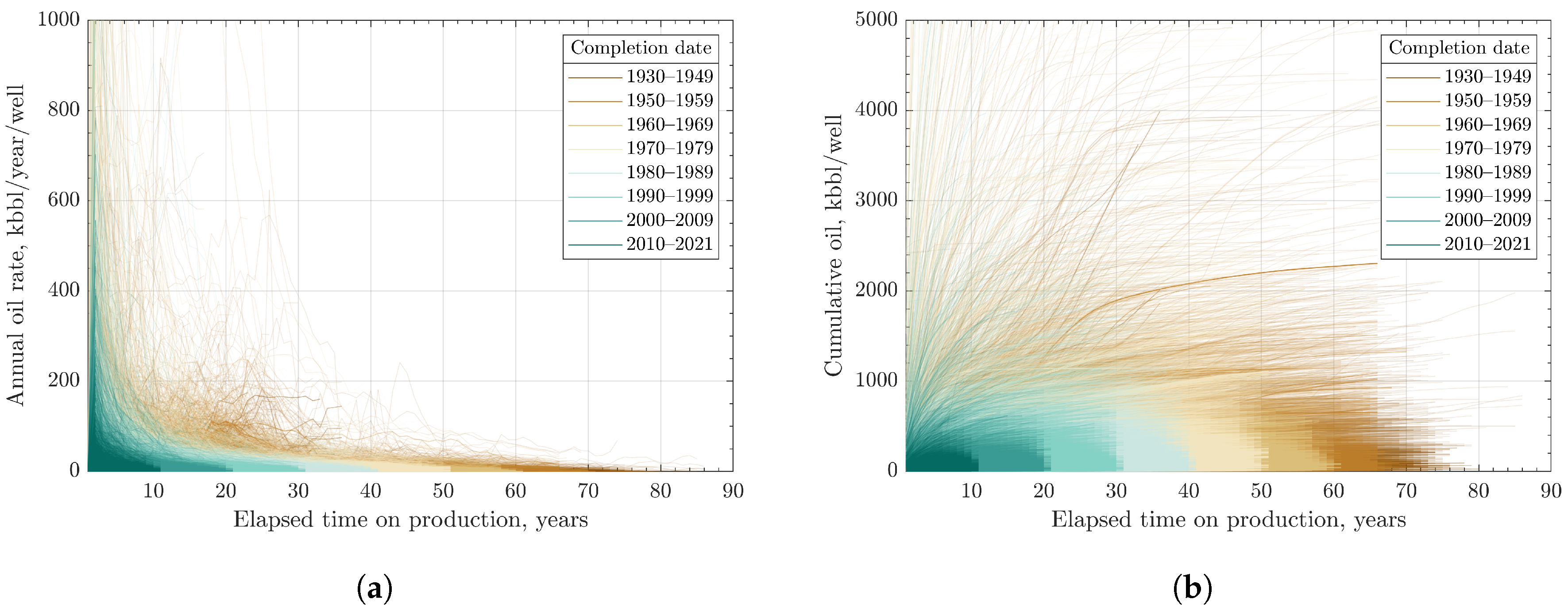
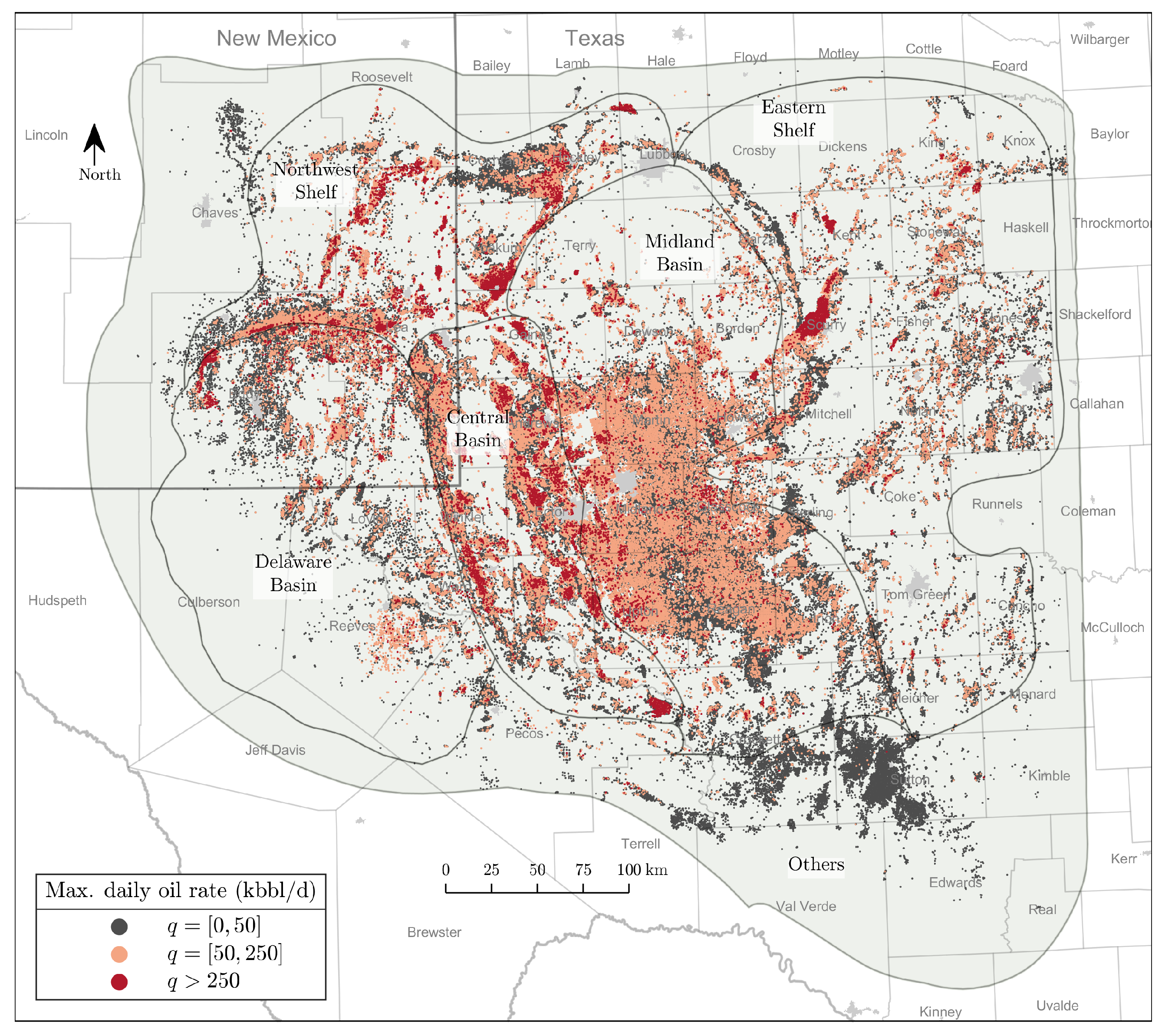
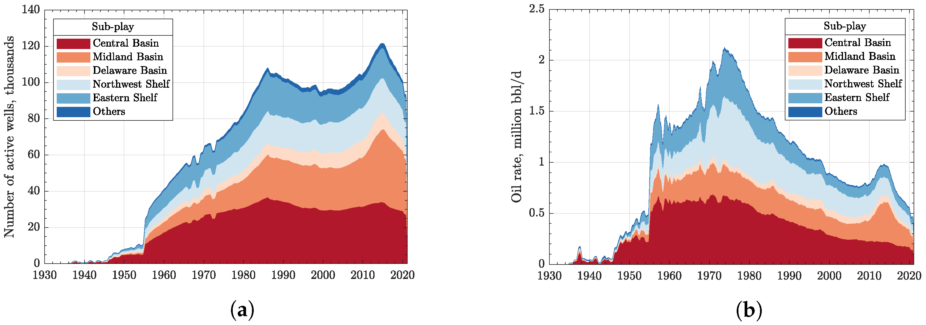
2.1. Exploratory Data Analysis

In Section 4, we explain that we obtained 484,759 well production time series from Enverus and FracFocus. This dataset is so massive that it cannot be loaded and analyzed as one file. Therefore, we conducted several exploratory data analyses to better visualize and understand the Permian Basin. In Figure 1, we plot the historical annual rate and cumulative oil production for each well. The individual well curves are colored-coded for eight completion date intervals. A quick inspection of these plots reveals that the old wells completed in the 1930s produced more annual oil than those completed recently. Furthermore, these old wells have survived for decades, while the new wells decline severely and cannot continue producing for decades.
In addition to the time series of the production data, we also have the surface well locations that we plot in Figure 2, Figure 3 and Figure 4. The light green overlay layer is the areal extent of the Permian Basin that we modified slightly from the USGS and EIA shape files. We further divide the entire basin into six sub-basins: (1) Central Basin, (2) Delaware Basin, (3) Midland Basin, (4) Northwest Shelf, (5) Eastern Shelf, and (6) Others. Similar to Figure 1, we color the map in Figure 2 based on the completion date intervals. We observe that the oldest wells in the 1930s were drilled in the Central Basin Platform, the Northwest Shelf, and the Eastern Shelf, which are shallower than the Delaware and Midland Basins. In contrast to the continuous (shale) reservoirs in which well locations are dispersed across each side of the basin, the well locations in the conventional reservoirs are spatially clustered and limited by the reservoir’s boundaries.
In the Permian, in fact, there are hundreds of different reservoirs, and it is difficult to analyze each one of them separately. Therefore we decided to cluster these reservoirs into several groups for which the geologic ages are relatively similar. Figure 3 shows four different reservoir ages in the Permian Basin: (1) the Guadalupian, (2) Leonardian, (3) Wolfcampian, and (4) Pre-Permian. Table 1 details the key reservoir layers that exist for each age. In geology, the age of a formation is often correlated with its depth. The reservoirs that are members of the Guadalupian, for instance, have an average age of 251 million years. These reservoirs are shallower than the Leonardian, Wolfcampian, and Pre-Permian formations.
In Figure 4, we show the spatial distribution of best and worst producing wells by coloring the data cloud with the maximum daily oil rates. Again, the best locations are clustered within the compact, small reservoir shapes. One can quickly tell that the Central Basin, Northwest Shelf, and Eastern Shelf contain more productive wells than the Others.
In Figure 5 and Figure 6, we plot the number of active wells and the total field–daily oil rate in the Permian. We use color to separate the contributions of each reservoir age or sub-play to total production. It appears that the Guadalupian has the highest number of producing wells, followed by the Leonardian. It is reasonable that the Guadalupian has the highest number of wells because it has the youngest, shallowest reservoirs, and it is cheaper to drill there. For the same reason, most wells are also drilled in the Central Basin, which is shallower than the other sub-plays.
The reservoir age corresponds to the bottomhole depths of the vertical wells, while sub-play corresponds to the surface locations (latitude and longitude) of each well. Both the reservoir age and sub-play accommodate vertical (z) and areal ( x × y ) spatial variability, while the completion date intervals accommodate temporal variations.

2.2. Design of Well Cohorts

From the exploratory data analysis in the previous section, we notice that production depends on each reservoir’s age, sub-play, and completion date intervals. Therefore, we design 192 spatiotemporal well cohorts detailed in Table 2. This division is important in that each well cohort is statistically stable, and the resulting well prototypes are not biased.

2.3. GEV Statistics and Historical Well Prototypes

As detailed in Section 4, we fit the annual well production with generalized extreme value (GEV) statistics to obtain the P 50 historical well prototypes. Figure 7 is an example of this procedure for all vertical wells in the Midland Basin sub-play with the Leonardian reservoir age and completed during 2000 to 2009. We first resample this well cohort into sub-groups with at least n years on production. In Figure 7, these sub-groups are shown as different rows; notice that each resampling reduces the number of samples, n. For each sub-group, we fit a GEV distribution into the empirical probability density function and obtain the location parameter, μ , scale parameter, σ , and the shape parameter, ξ .
For comparison, we also show the lognormal distribution fits to show the superiority of the GEV for annual production data. We notice that the histogram for each new row shifts to the left, showing the decline of annual oil production. Therefore, we should also expect that the values of μ , mean in Equation (3), P 10 , and P 90 will shift to smaller values. The shape parameter ξ varies between 0.19 and 0.29 > 0 , selecting for Fréchet distribution, consistently with our prior analyses of other petroleum basins [13,16,19,22]. Finally, we connect each GEV mean of every n-th year subgroup to construct the historical well prototype.

2.4. Physical Scaling and Extended Well Prototypes

We repeat the procedure illustrated in Figure 7 for each cohort and obtain 192 historical well prototypes shown as solid colored lines in Figure 8. As each prototype is created from historical data, it is bounded from above by t max years on elapsed production time. Therefore, to predict a prototype’s production at longer times, we apply the physical scaling method detailed in Section 4 and derived in Appendix A. As a result, we obtain the extended well prototypes, valid for up to a century, and shown as the dashed colored lines in Figure 8. The matching parameters, τ and M , from all 192 well cohorts are then fitted by GEV, and lognormal distributions shown in Figure 9. The GEV means of τ and M are 2.37 years and 106.37 ktons, respectively.

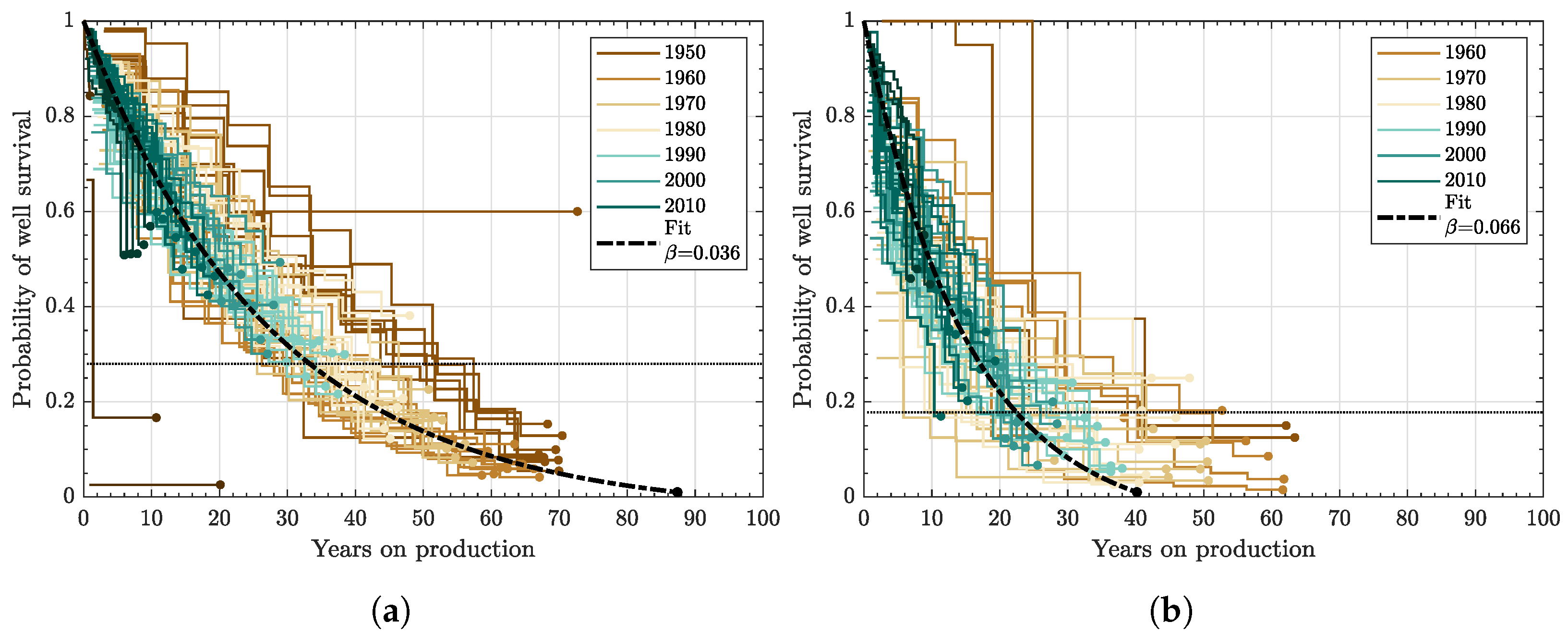
2.5. Probability of Well Survival

In Figure 8, we see an ideal condition that the oil production can last for 10 decades. In reality, many factors such as well integrity, sand production, water influx, permeability reduction, etc., might cause irreversible damage to the wells. When their production becomes uneconomic, operators shut-in the wells immediately. We calculate the probability of well survival for each region (sub-play × reservoir age) in the Permian, detailed in Section 4. Using Equation (A28), we fit each probability of survival (see, e.g., Figure 10). The zero-probability intercepts of the fits determine the maximum times of well survival, t surv . Table 3 summarizes t surv results for each Permian region.

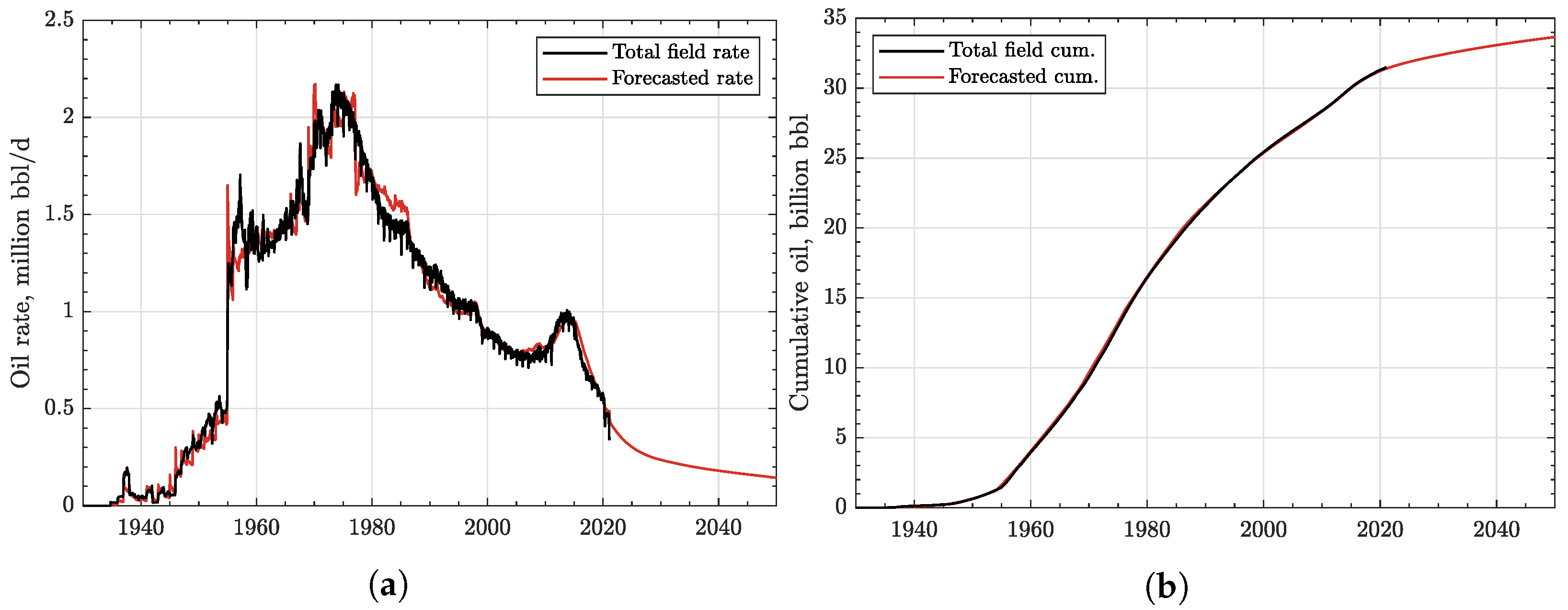
2.6. Total Field Forecast

We replace historical production from each of the existing 484,759 vertical wells in the Permian with the corresponding well prototypes, time-shift the prototypes, and sum them up to obtain total field production forecast. In Figure 11, the black lines show the historical total field production, while the red lines are the forecasted rate and cumulative oil obtained from summation of the well prototypes. At this stage, we confirm that our well prototypes are robust, and the forecast matches the historical production rather remarkably. From the cumulative plot, we posit that the estimated ultimate recovery from the 484,759 existing wells in the Permian will be about 34 billion barrels by 2050.

3. Discussion

We have generated the physics-guided, data-driven forecasts for all 484,759 vertical wells in the Permian. Our well prototypes are robust, match historical production, and give a smooth, least-squares-optimal estimate of future production for several more decades. One can use these unbiased well prototypes in Figure 8 to compare productivity variations among the different reservoir ages, sub-plays, and completion date intervals. The most notable comparison is that the average ultimate recovery has steadily declined with time. One can also infer that the rate of finding big conventional reservoirs has been declining drastically since the 1970s. In contrast, as shown in Figure 12, operators today need to drill wells that are two times deeper than the 1930s’ wells and produce 4–12 times less than their predecessors.
From Figure 8, we also see that the older the reservoir’s age, the higher the ultimate recovery is. However, in Table 3, the older the reservoir’s age, the faster the well failure rate is. This may be related to the depth-dependent well integrity problems and/or permeability reduction due to severe rock compaction. We can also infer that in terms of well productivity and survival time, the Central Basin has been the best location to drill vertical wells ever since the 1930s. This is related to the geological fact that the Central Basin is a carbonate platform that separates Midland and Delaware Basins. We can expect that a carbonate reservoir in this area has the best porosity and permeability among other sub-plays of Permian. In addition, it is relatively shallower, so that drilling therein is less expensive. However, unlike unconventional reservoirs where hydrocarbons are spread continuously across the vast shale extents, the conventional reservoirs, such as those in Central Basin, are compact and limited in size. Unfortunately, the best well locations have been drilled massively for a century. Today, operators are left with drilling and hydraulically fracturing the unconventional shale plays to maintain the high production rate we discuss in a separate paper.

4. Materials and Methods

We mined public well data in the Permian from Enverus database and FracFocus. As of February 2021, there were 562,416 wells completed in the Permian Basin (Texas and New Mexico). From these wells, we have retained only 484,759 vertical wells that were completed in conventional reservoirs. The remaining hydraulically fractured horizontal or directional wells completed in unconventional shale reservoirs are analyzed in a separate paper [29]. The approach we used here is rooted in our prior work on the physics-guided, data-driven forecasts in the Barnett [13], Eagle Ford [15], Bakken [16,17], Haynesville [19], and Marcellus [22]. Our approach is as follows:
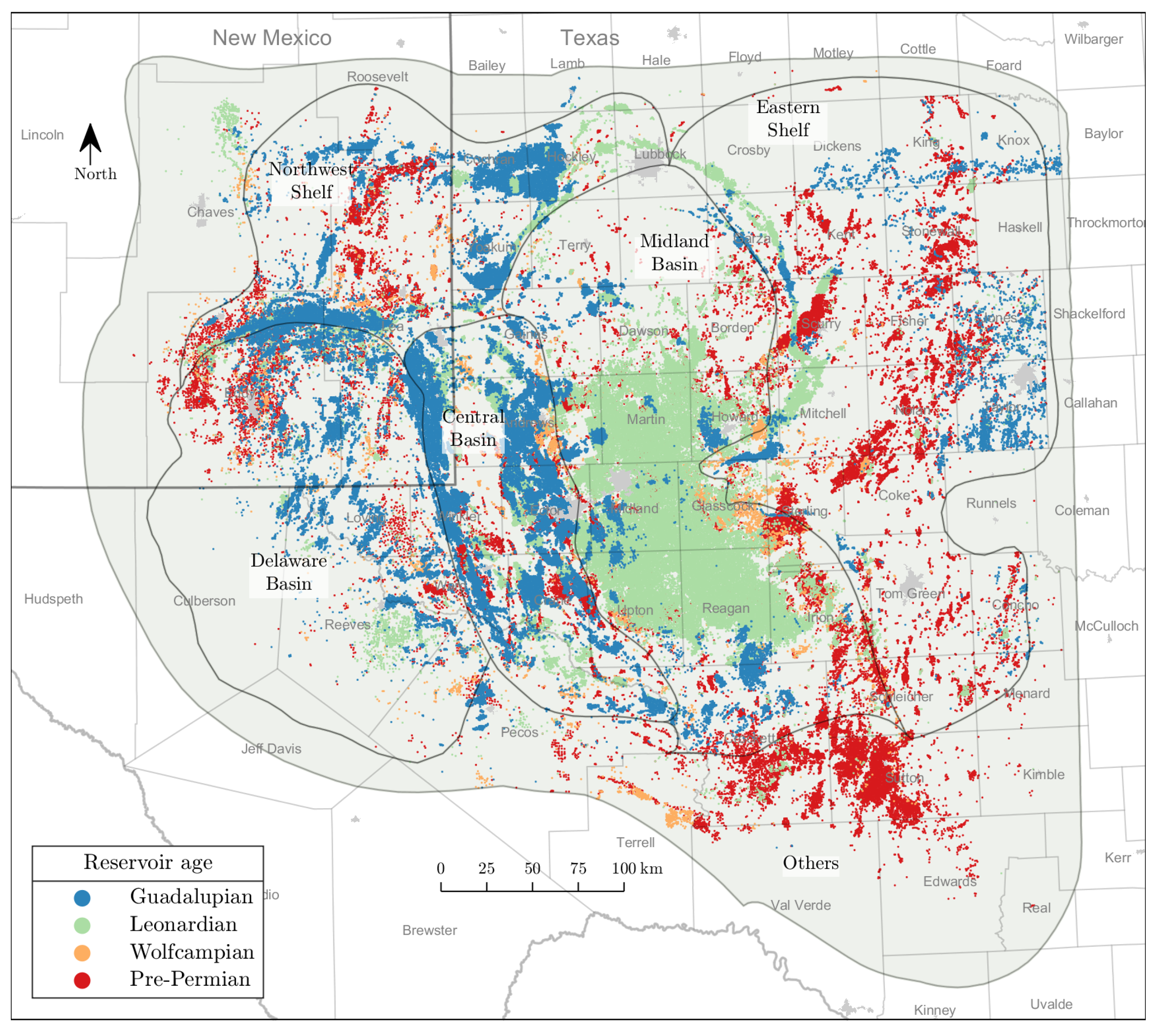
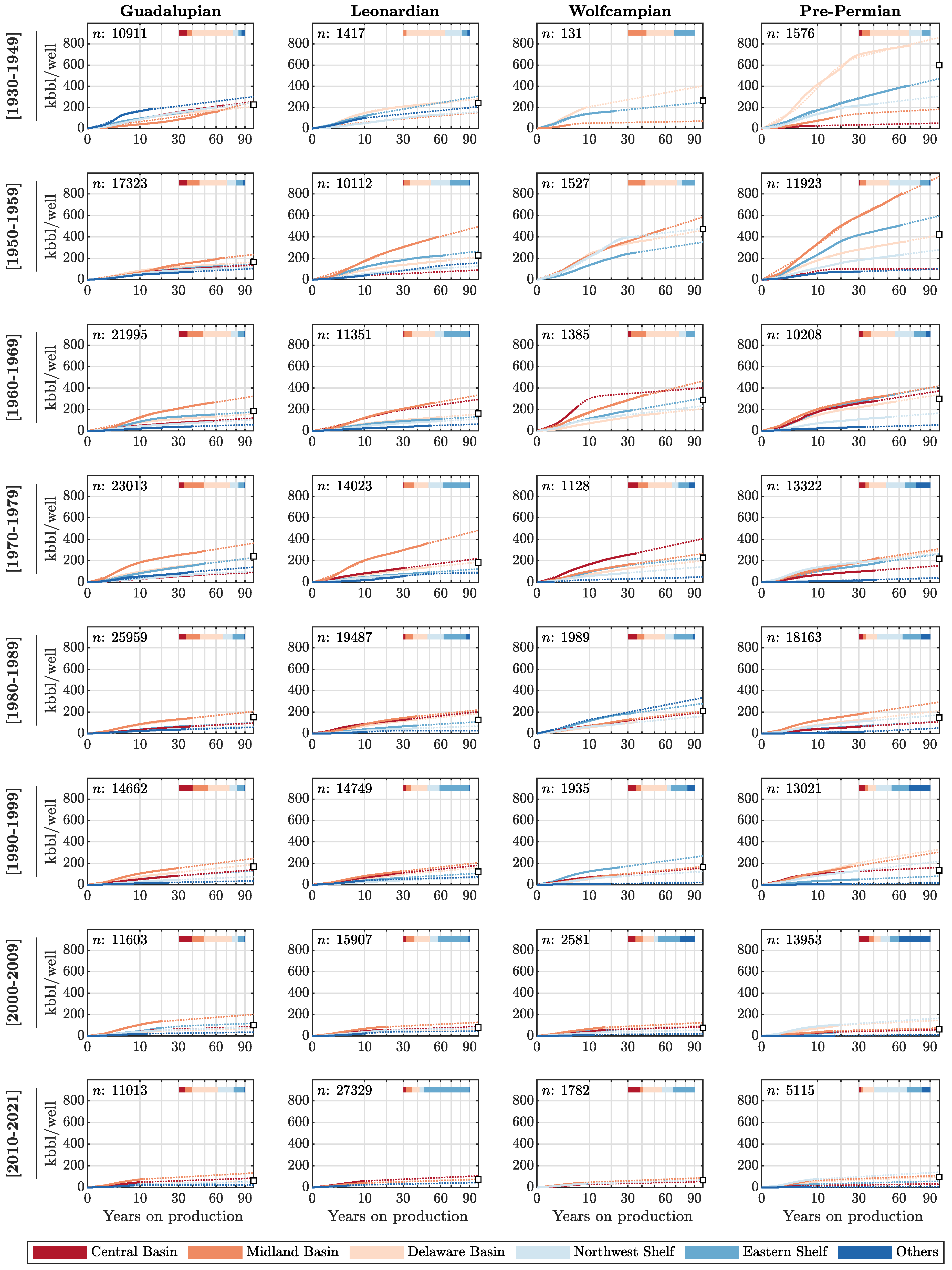
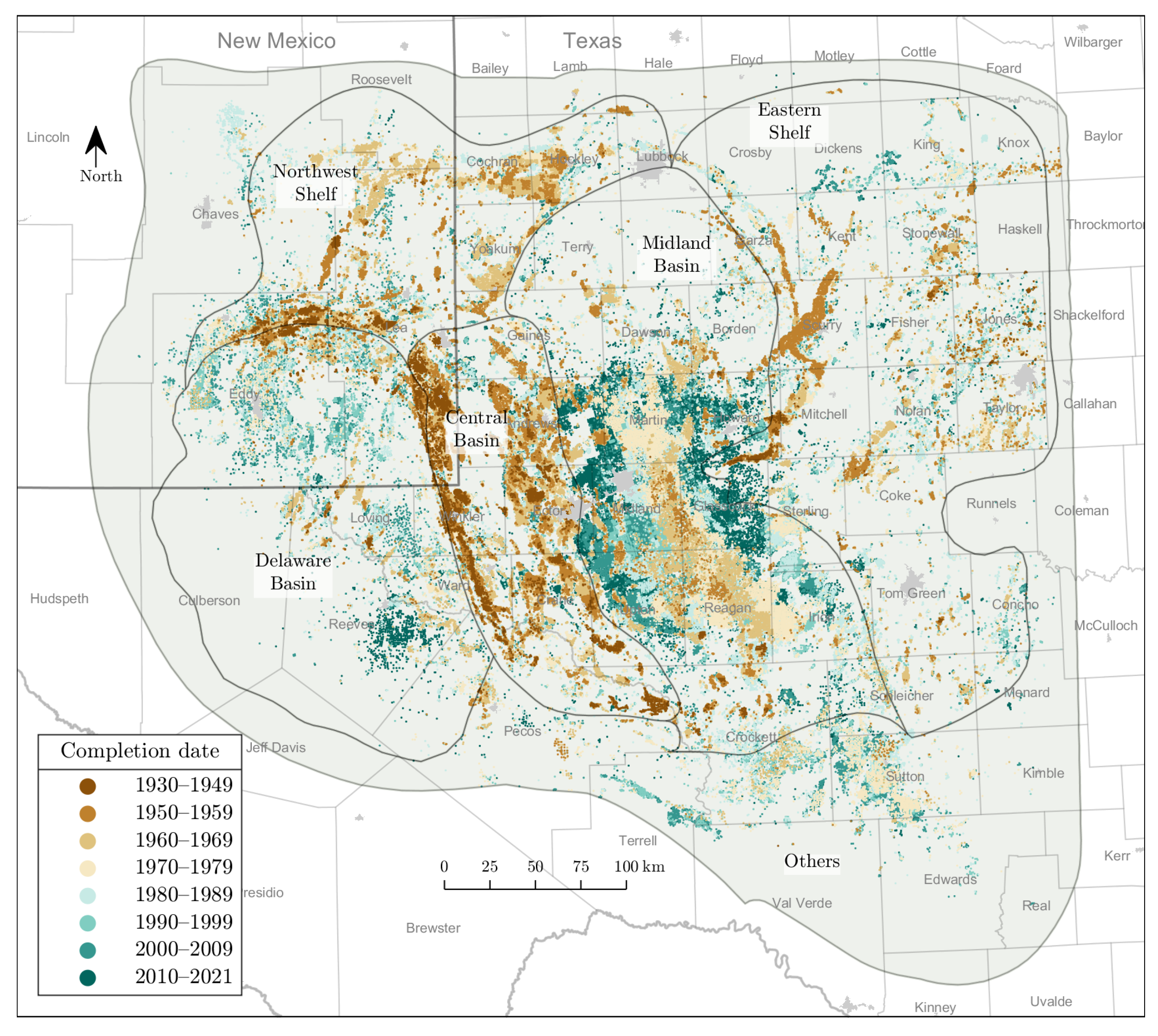
  • Design of well cohorts: We divide nearly half a million vertical wells in the Permian into 192 spatiotemporal well cohorts. The number 192 is the multiplication of four reservoir ages, six sub-plays, and eight completion date intervals detailed in Table 2.
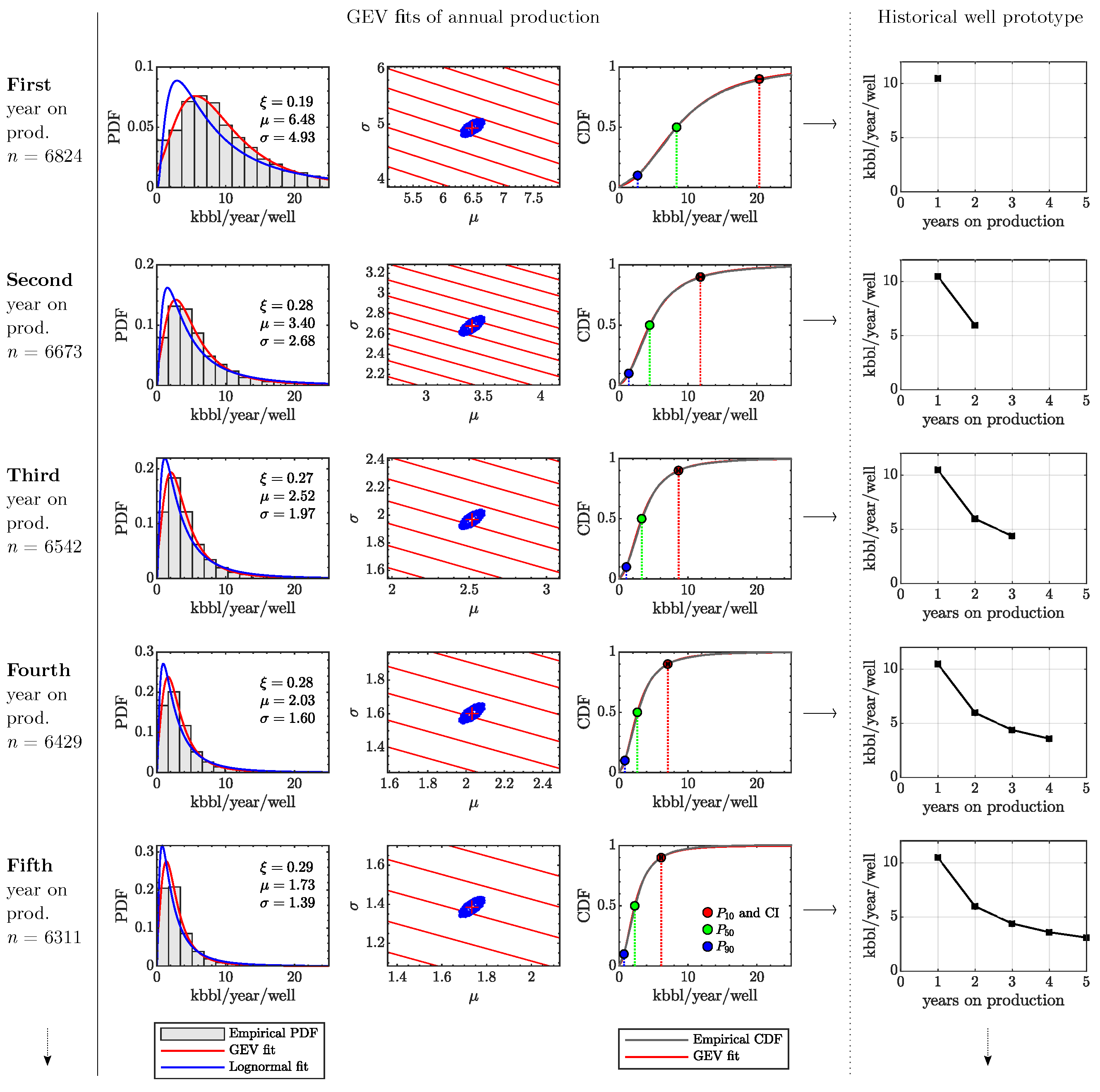
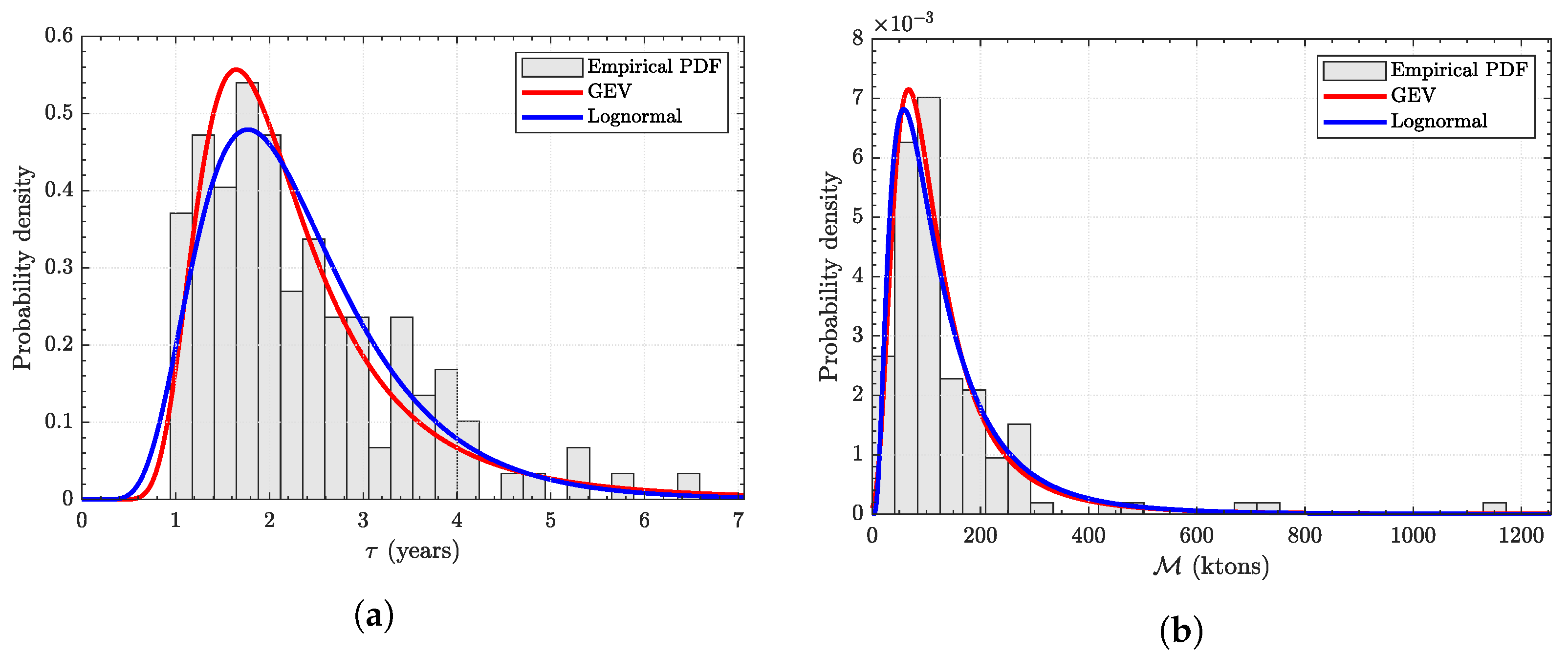
  • Perform GEV statistics and historical well prototypes: For each cohort, we sample i = 1 , 2 , , n years on production and fit a generalized extreme value distribution using Equation (1) to find the location parameter, μ , scale parameter, σ , and shape parameter, ξ . Using Equations (2) and (3), we calculate the expected value or mean, P 50 , the upper bound, P 10 , and the lower bound, P 90 , of the GEV distributions. We then connect each value of annual P 50 ’s to construct a historical well prototype, see Figure 7.
    PDF : f ( x ) = 1 σ 1 + ξ x μ σ 1 ξ 1 e 1 + ξ x μ σ 1 ξ
    CDF : F ( x ) = e 1 + ξ x μ σ 1 ξ
    Mean : E ( x ) = μ σ ξ + σ ξ Γ ( 1 ξ ) , ξ 0 .
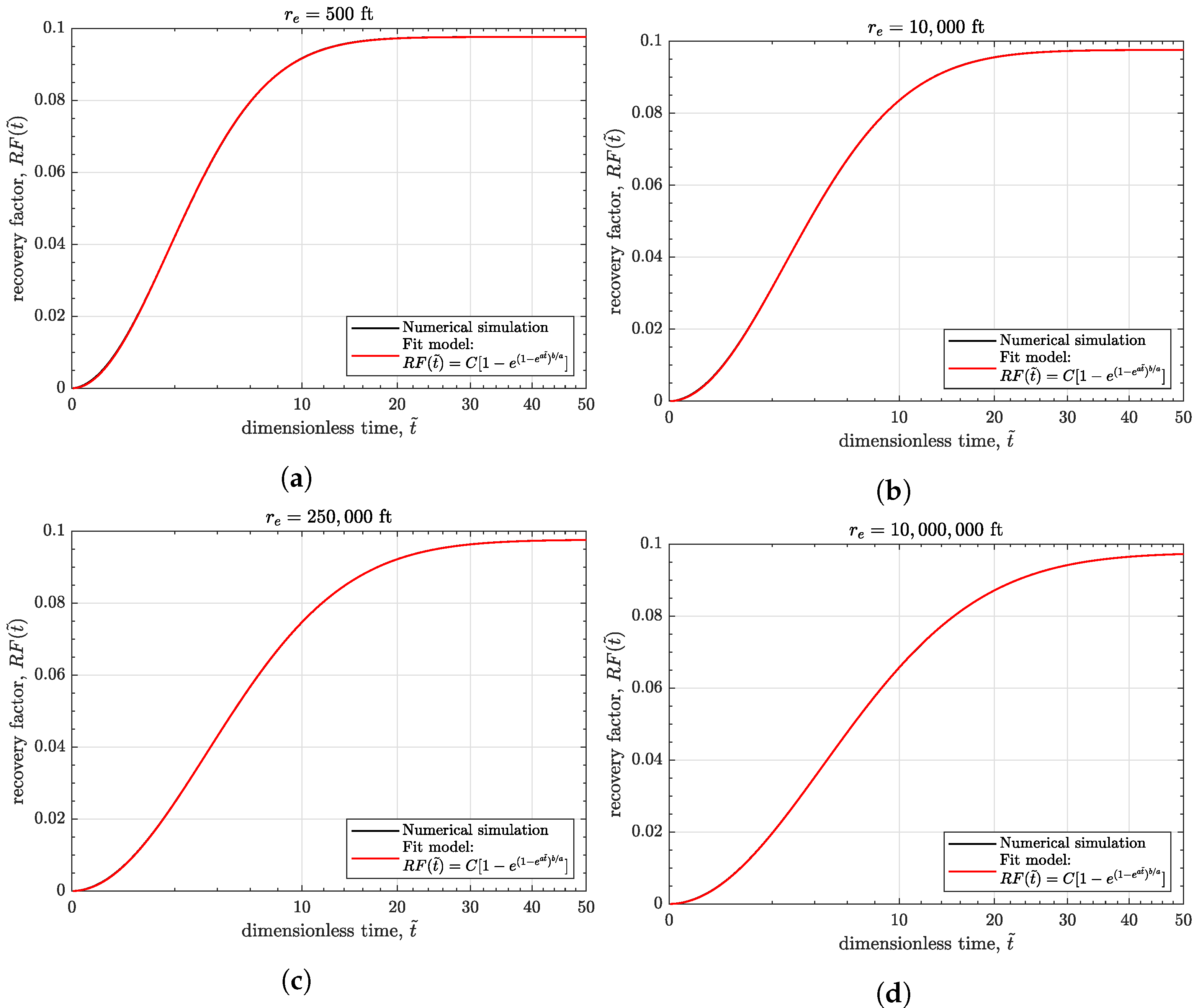
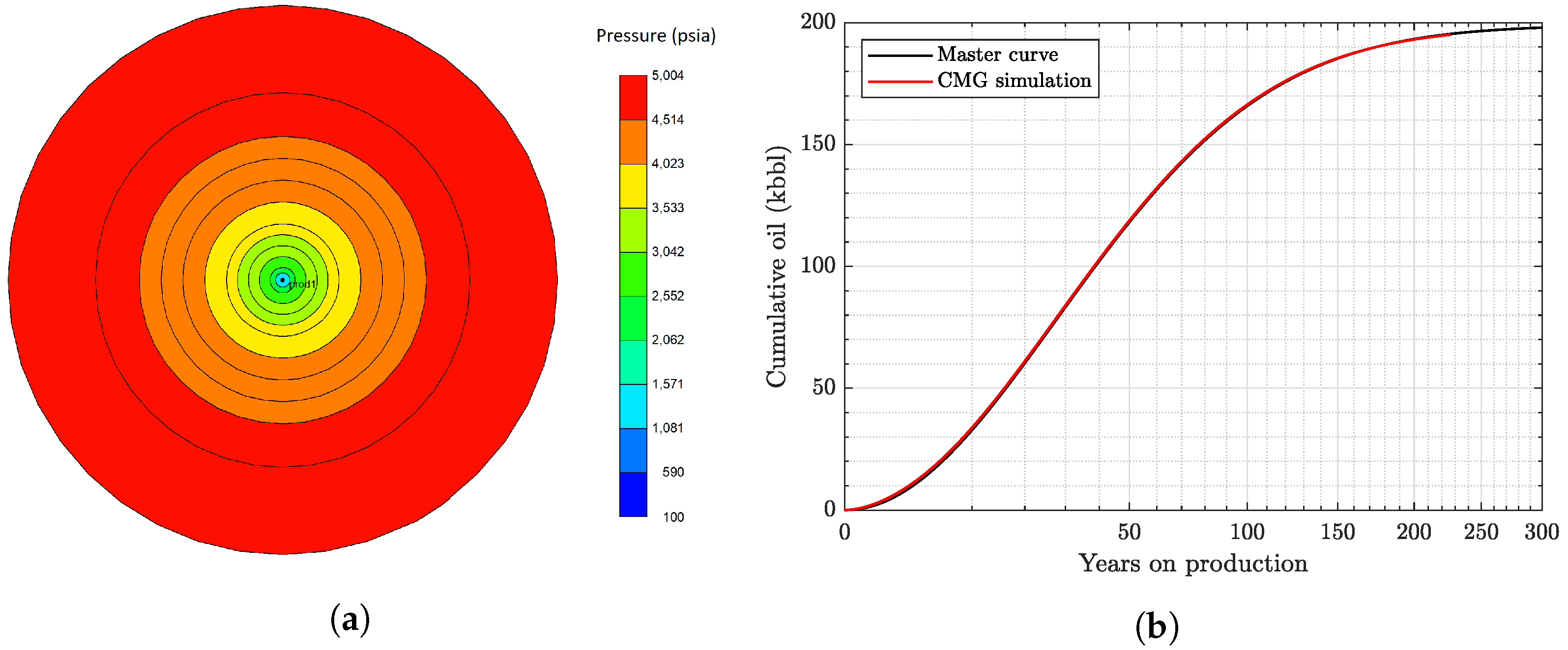
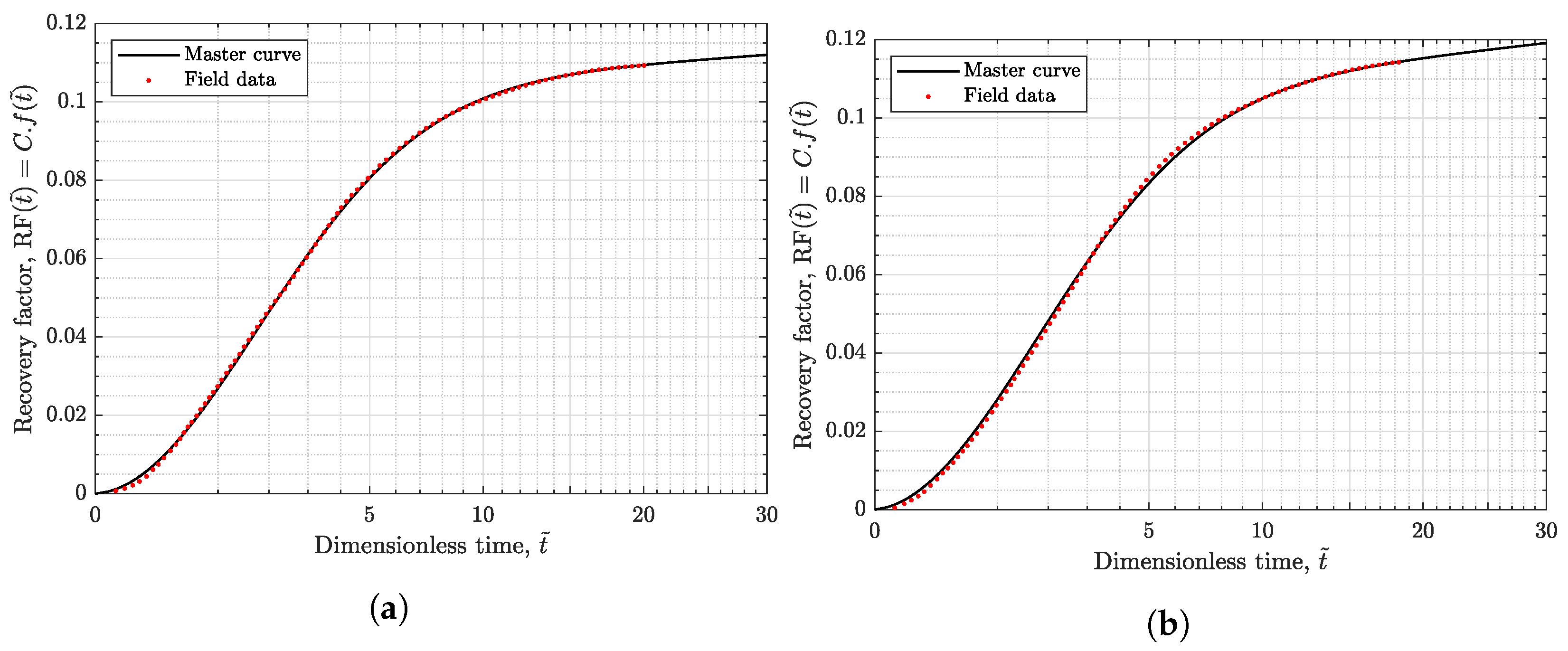
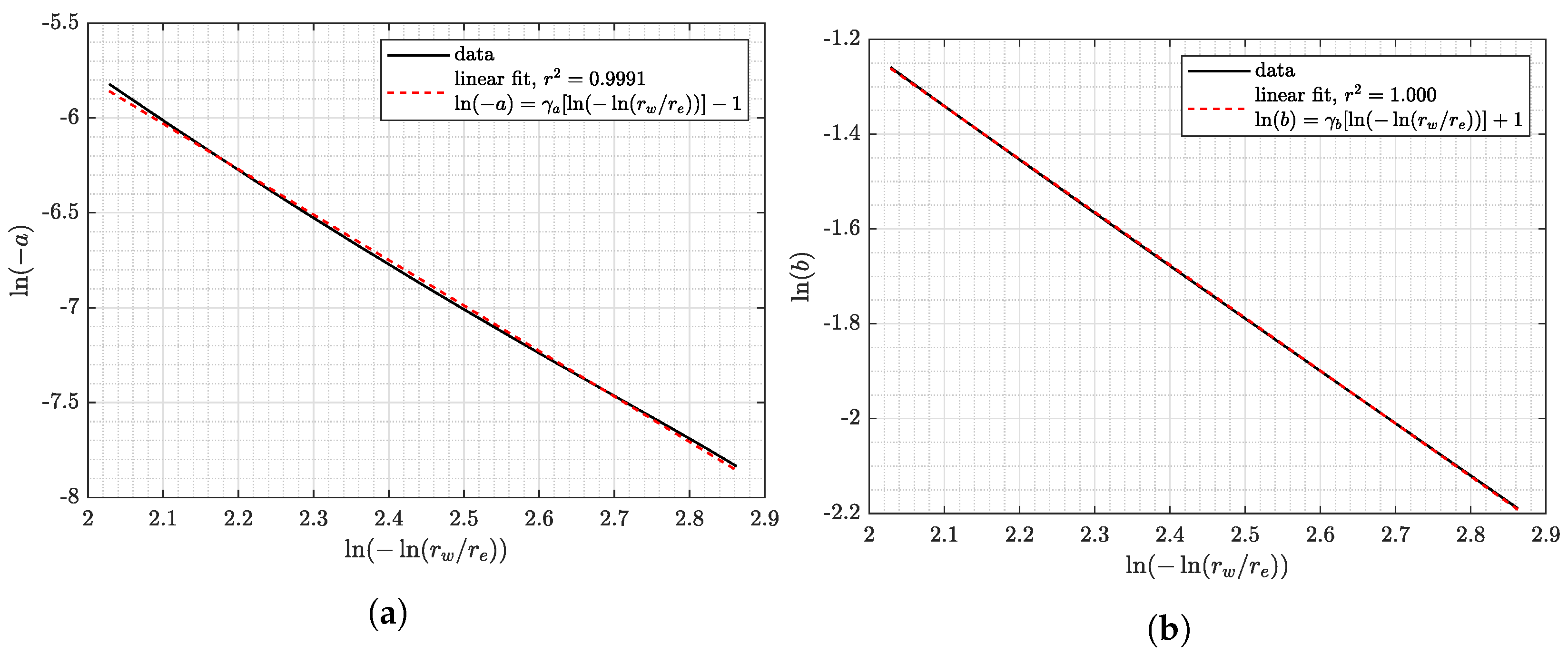
  • Perform physical scaling and extended well prototypes: We use the physical scaling approach to extend the historical well prototypes for several more decades. In Appendix A, we derive the new physical scaling for conventional vertical wells. First, we convert the annual oil rate into the cumulative mass produced using Equation (A31). Next, we scale the cumulative mass with τ along the x-axis and by M along the y-axis, so that the scaling result matches the master curve in Equation (A34).
  • Estimate probability of well survival: We calculate the survival probability of each sub-region of the Permian using Equation (4), where N active , i and N inactive , i are the numbers of active and inactive wells in year-i:
    P survival , i = N active , i N active + N inactive , i
    To estimate the maximum time of well survival, we fit the probability of survival with Equation (5) and find the intercept of the curve fit to the probability equal to zero:
    y ( t ) = ( 1 + β ) ( e t β β )
  • Complete total field forecast: We replace the actual reported field production rate from all existing vertical wells in the Permian with the corresponding extended well prototypes. The summation of all prototypes becomes the total basin-wide forecast of the conventional Permian wells.

5. Conclusions

  • We have provided a transparent hybrid method of forecasting conventional oil production at a basin scale.
  • A combination of GEV statistics of very large data sets with physical scaling matches historical production data almost perfectly and gives a smooth, optimal prediction of the future in the least-square sense.
  • Our spatiotemporal well cohorts are a combination of different reservoir ages, sub-plays, and completion date intervals.
  • The estimated ultimate recovery (EUR) from all 484,759 existing vertical wells in the Permian is about 34 billion barrels of oil.
  • We observed that the vertical wells in the Permian can last between 10 and 100 years, depending on which sub-play and reservoir these wells penetrate.
  • In practice, no large reservoir has been found in the Permian since the 1970s.
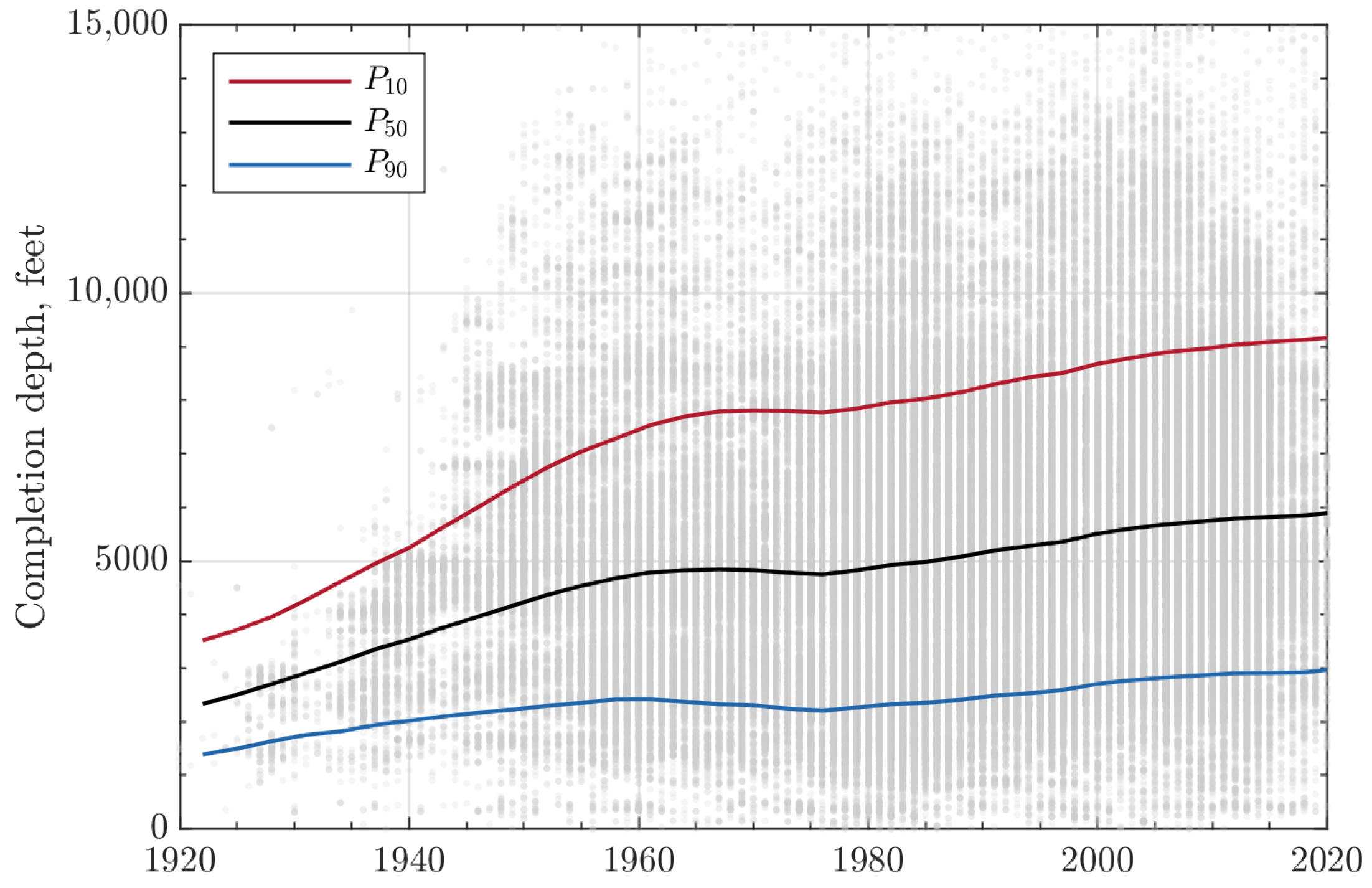
  • Today, operators need to drill wells that are twice as deep as the 1930s’ wells but that produce 4–12 times less.

Author Contributions

Conceptualization, T.P. and W.S.; methodology, T.P. and W.S.; software, W.S. and T.P.; validation, T.P. and W.S.; formal analysis, W.S. and W.K.; investigation, W.K. and W.S.; resources, T.P.; data curation, W.K.; writing—original draft preparation, W.S.; rewriting manuscript—review and editing, T.P. and W.S.; visualization, W.S.; supervision, T.P. and W.K.; project administration, T.P.; funding acquisition, T.P. All authors have read and agreed to the published version of the manuscript.

Funding

Wardana Saputra (PhD student) was supported by baseline research funding from KAUST to Tad Patzek. Wissem Kirati (Research Engineer) was supported by the Division of Computer, Electrical and Mathematical Science at KAUST.

Acknowledgments

The authors thank the Ali I. Al-Naimi Petroleum Engineering Research Center (ANPERC) at KAUST for supporting this research. We thank the reviewers for their thorough, informative and timely reviews.

Conflicts of Interest

The authors declare no conflict of interest.

Abbreviations

The following abbreviations are used in this manuscript:
EUREstimated Ultimate Recovery
GEVGeneralized Extreme Value
GORGas to Oil Ratio
ODEOrdinary Differential Equation
PDEPartial Differential Equation
RFRecovery Factor

Appendix A. Physical Scaling for Conventional Wells

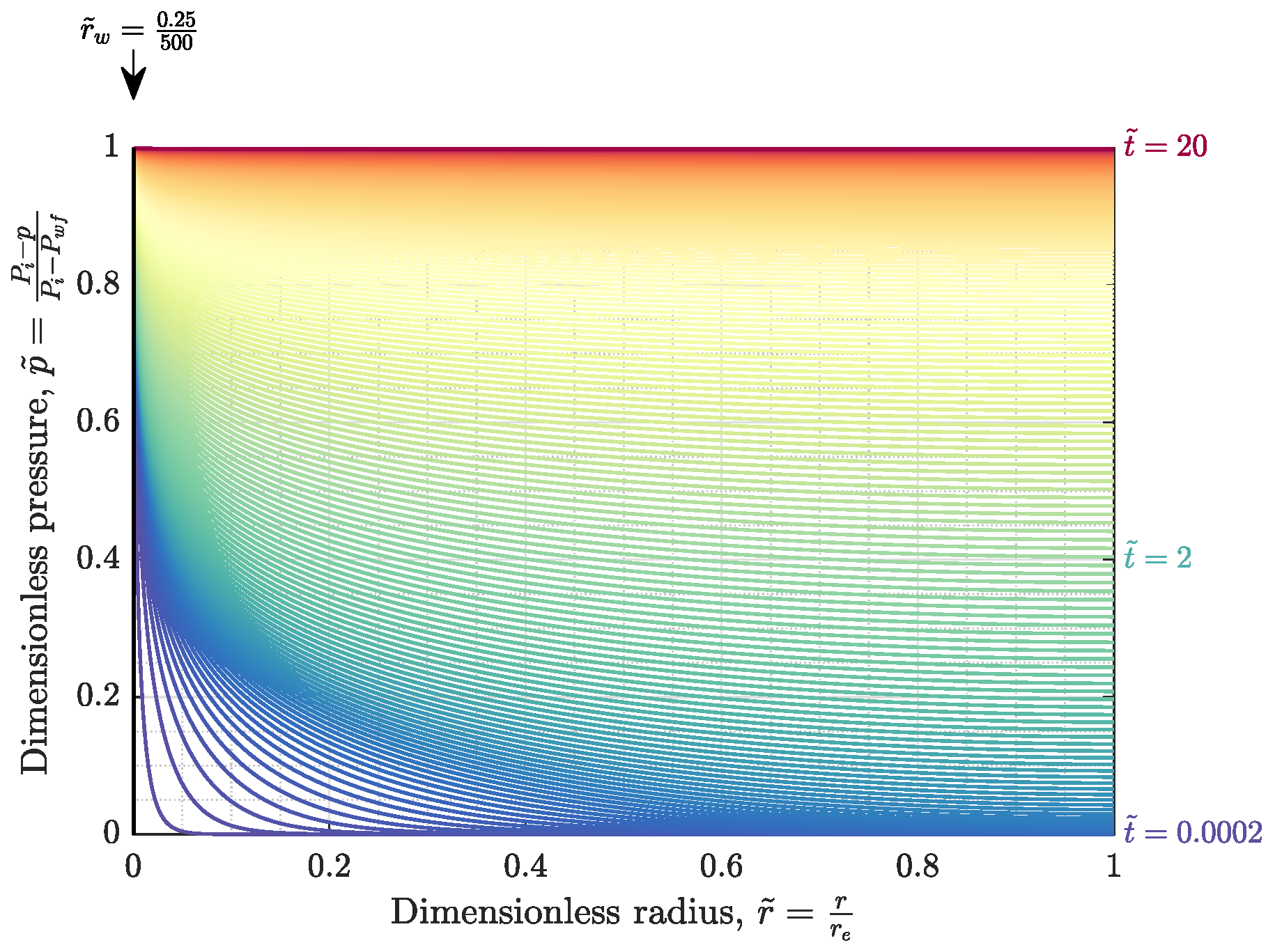
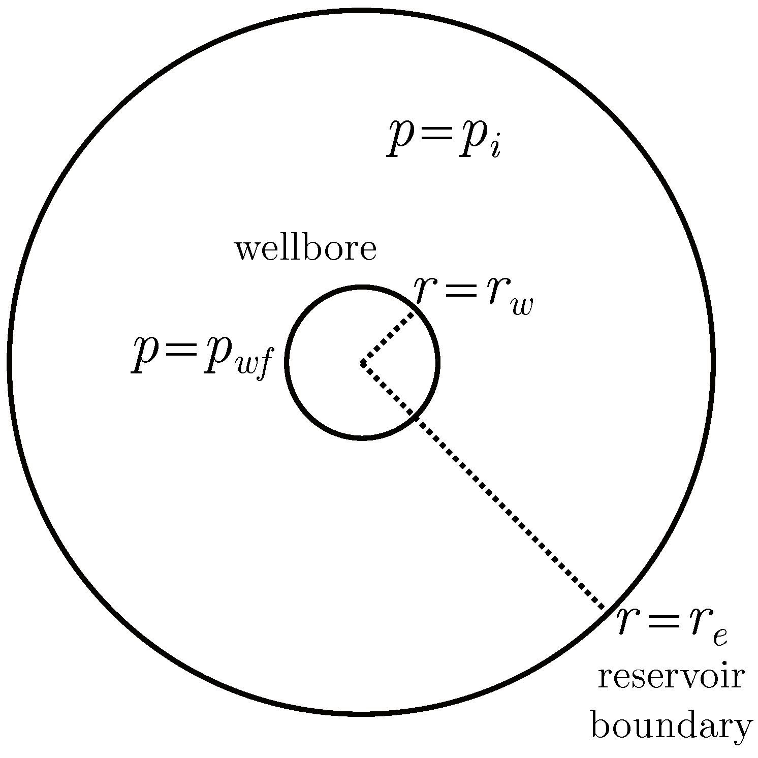
Appendix A.1. One-Dimensional Pressure Diffusion Equation in Radial Coordinates: Constant Pressure—Bounded Reservoir

We begin with a simple model of radial oil flow from a bounded reservoir with radius, r e , towards the wellbore with radius, r w , see Figure A1. The initial reservoir pressure is P i , and the pressure at the wellbore is kept constant at P w f .
Figure A1. A simple model of radial flow—constant pressure—bounded reservoir.
Energies 15 00904 g0a1
For the system described in Figure A1, pressure diffuses radially following a parabolic partial differential equation:
p t = α ( p ) 1 r r r p r
where p is pressure, t is time, r radius, and α ( p ) is the hydraulic diffusivity coefficient:
α ( p ) = k ϕ c t μ o ρ o ρ fluid , i
where, k is the average rock permeability, ϕ is the porosity, c t is the total system (oil and pore space) compressibility, μ o and ρ o are the oil viscosity and density, and the initial bulk fluid density is ρ fluid , i . The initial and boundary conditions for this mathematical problem (IBVP) of uniform initial reservoir pressure and bounded reservoir are listed in Equation (A3):
p ( r , t = 0 ) = P i p ( r = r w , t ) = P w f p r r = r e = 0
To solve the IBVP in Equations (A1)–(A3), we render it dimensionless by introducing the dimensionless pressure, p ˜ , time, t ˜ , and radius, r ˜ :
p ˜ = P i p P i P w f t ˜ = α i r e 2 t r ˜ = r r e
By substituting Equation (A4) into Equations (A1) and (A2), we obtain the following dimensionless pressure diffusion equation:
p ˜ t ˜ = 1 r ˜ r ˜ r ˜ p ˜ r ˜
and the following initial and boundary conditions:
p ˜ ( r ˜ , t ˜ = 0 ) = 0 p ˜ ( r ˜ = r ˜ w , t ˜ ) = 1 p ˜ r ˜ r ˜ = 1 = 0
If a reservoir is infinite-acting (unbounded), one can apply the Boltzmann transformation [30] by substituting η = r ˜ 2 4 t ˜ into Equation (A5). Using this approach, a partial differential diffusion equation, a PDE, can be converted into an ordinary differential equation, an ODE. The solution of this ODE is in the form of exponential integral, E i ( x ) , function.
Unfortunately, this similarity solution of the pressure diffusion equation does not work for a bounded reservoir [31]. To solve the complicated constant-pressure, bounded-reservoir problem in Equations (A5) and (A6), early pioneers [32,33,34] used the Laplace transform approach. However, the solution is a Fourier–Bessel series in the complex domain, and at the end, one must resort to a numerical inversion of the Laplace transform by, e.g., Mellin’s inversion formula.
In this work, we solve the PDE numerically and develop a user-friendly semi-analytical solution of Equations (A5) and (A6) for arbitrary reservoir radii, r e .

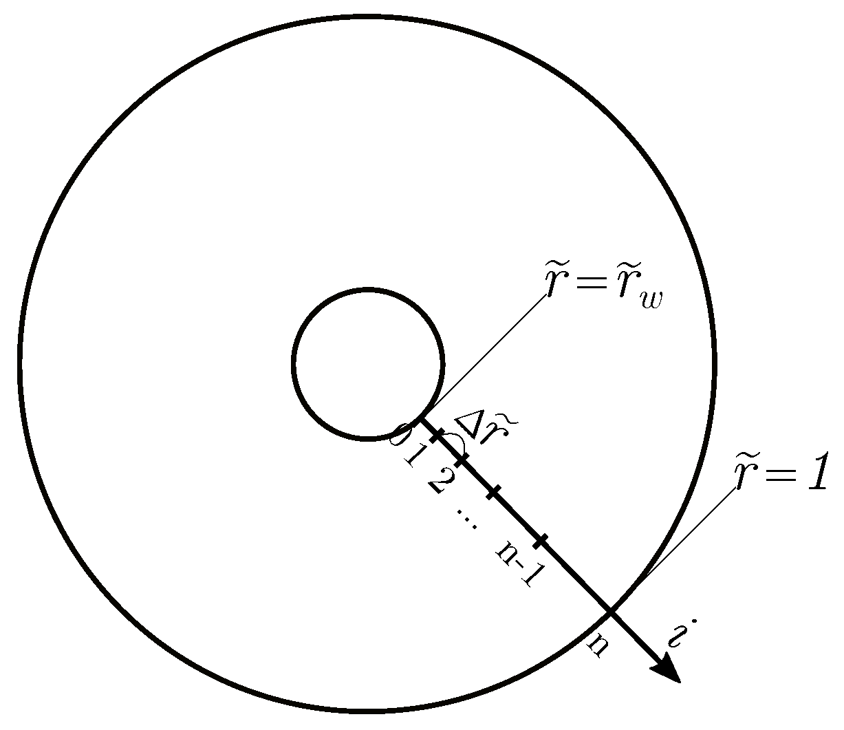
Appendix A.2. Discretization Techniques and Numerical Solutions

A second-order PDE can be solved using a finite difference method, e.g., with a central differencing scheme. However, the PDE in Equation (A5) is highly non-linear and needs to be modified for better numerical stability. Let us define u = ln ( r ˜ ) , therefore:
u = ln ( r ˜ ) r ˜ = e u d u d r ˜ = 1 r ˜ = 1 e u d r ˜ = e u d u
and substitute Equation (A7) into Equation (A5):
p ˜ t ˜ = 1 r ˜ r ˜ r ˜ p ˜ r ˜ p ˜ t ˜ = 1 e u e u u e u p ˜ u d u d r p ˜ t ˜ = 1 e 2 u u e u p ˜ u 1 e u p ˜ t ˜ = e 2 u 2 p ˜ u 2
Figure A2 illustrates a discretization of the radial coordinate. i = 0 is located at the wellbore, r ˜ = r ˜ w , and i = n corresponds to the reservoir outer radius, r ˜ = 1 . Applying an implicit finite central differencing scheme to Equation (A8), we obtain:
p ˜ i t ˜ + 1 p ˜ i t ˜ Δ t ˜ = e 2 u p ˜ i + 1 t ˜ + 1 p ˜ i t ˜ + 1 u i + 1 u i p ˜ i t ˜ + 1 p ˜ i 1 t ˜ + 1 u i u i 1 u i + 1 2 u i 1 2
Substitute back u = ln r ˜ to Equation (A9) to obtain:
p ˜ i t ˜ + 1 p ˜ i t ˜ Δ t ˜ = r ˜ 2 p ˜ i + 1 t ˜ + 1 p ˜ i t ˜ + 1 ln r i + 1 r i ln r i + 1 2 r i 1 2 p ˜ i t ˜ + 1 p ˜ i 1 t ˜ + 1 ln r i r i 1 ln r i + 1 2 r i 1 2
Equation (A10) can be simplified as:
a i p ˜ i 1 t ˜ + 1 + b i p ˜ i t ˜ + 1 + c i p ˜ i + 1 t ˜ + 1 = p ˜ i t ˜
where a i , b i , and c i are calculated as follows:
a i = Δ t ˜ r ˜ i 2 ln r i r i 1 ln r i + 1 2 r i 1 2 b i = 1 Δ t ˜ r ˜ i 2 ln r i r i 1 ln r i + 1 2 r i 1 2 + r ˜ i 2 ln r i + 1 r i ln r i + 1 2 r i 1 2 c i = Δ t ˜ r ˜ i 2 ln r i + 1 r i ln r i + 1 2 r i 1 2
In Equation (A6), the first boundary condition, p ˜ ( r ˜ = r ˜ w , t ˜ ) = 1 , corresponds to a Dirichlet problem. Substitute p ˜ 0 t ˜ + 1 = 1 to Equation (A11):
a 1 ( 1 ) + b 1 p ˜ 1 t ˜ + 1 + c 1 p ˜ 2 t ˜ + 1 = p ˜ 1 t ˜ b 1 p ˜ 1 t ˜ + 1 + c 1 p ˜ 2 t ˜ + 1 = p ˜ 1 t ˜ a 1
The second boundary condition, p ˜ r ˜ r ˜ = 1 = 0 , corresponds to a Neumann problem. Substitute p ˜ n + 1 t ˜ + 1 = p ˜ n t ˜ + 1 to Equation (A11):
a n p ˜ n 1 t ˜ + 1 + b n p ˜ n t ˜ + 1 + c n ( p ˜ n t ˜ + 1 ) = p ˜ n t ˜ a n p ˜ n 1 t ˜ + 1 + ( b n + c n ) p ˜ n t ˜ + 1 = p ˜ n t ˜
Together, Equations (A11)–(A14) can be written in the following matrix and vector notation:
b 1 c 1 a 2 b 2 c 2 a n 1 b n 1 c n 1 a n [ b n + c n ] X p ˜ 1 t ˜ + 1 p ˜ 2 t ˜ + 1 p ˜ n 1 t ˜ + 1 p ˜ n t ˜ + 1 P new = p ˜ 1 t ˜ a 1 p ˜ 2 t ˜ p ˜ n 1 t ˜ p ˜ n t ˜ P old
Inverting this problem, pressure at each time step can be obtained implicitly as follows:
P new = X \ P old
Figure A2. Discretization in radial direction.
Energies 15 00904 g0a2
Figure A3 shows the numerical solution of Equation (A5) with the initial and boundary conditions in Equation (A6).
Figure A3. Numerical solution of the radial pressure diffusion for constant pressure—bounded reservoir ( r e = 500 ft).
Energies 15 00904 g0a3

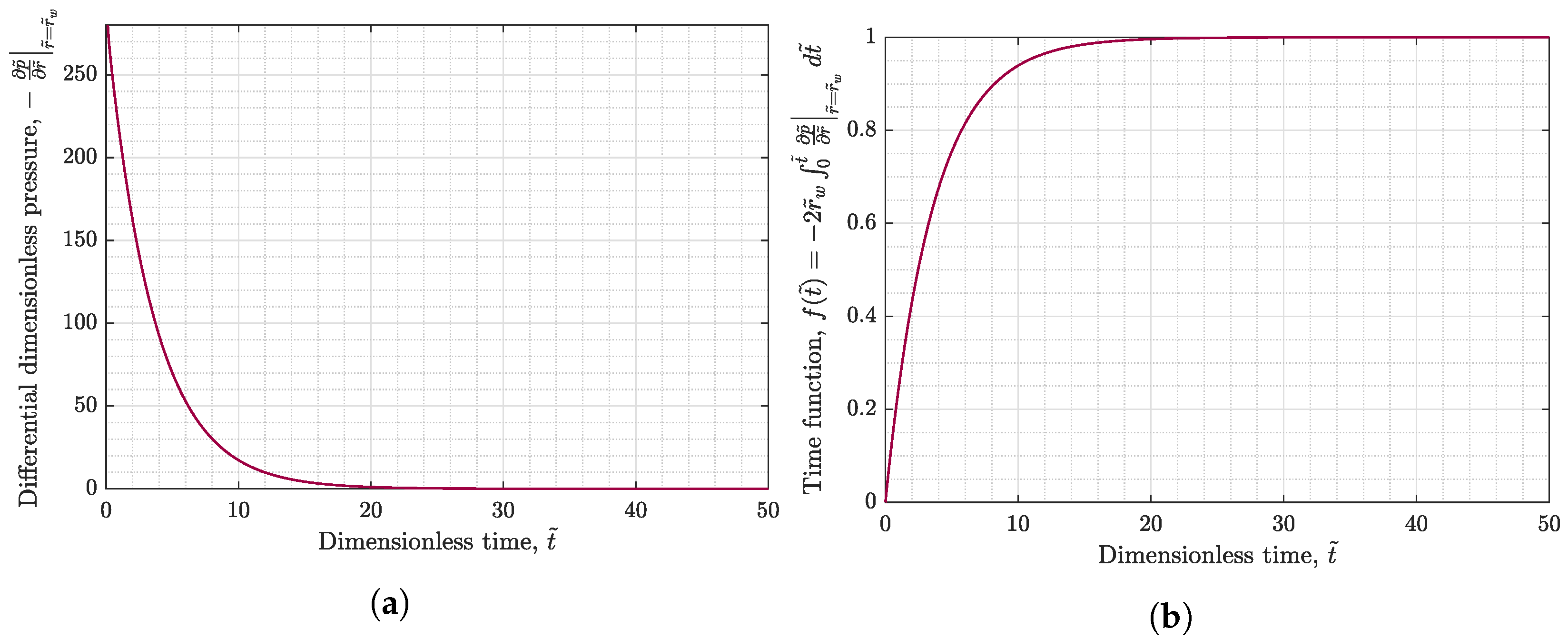
Appendix A.3. Calculating Recovery Factor

Recall Darcy’s equation [35,36] toward a wellbore with the radius, r w , formation thickness, h, and the surface area, 2 π r w h :
q = k 2 π r w h μ p r r = r w
Substitute the dimensionless pressure and radius from Equations (A4)–(A17):
q = k 2 π r w h μ P i P w f r e p ˜ r ˜ r ˜ = r ˜ w q = ( P i P w f ) 2 π k h μ r ˜ w p ˜ r ˜ r ˜ = r ˜ w
We now introduce a characteristic pressure interference time, τ , which is the time needed for the pressure to diffuse to the reservoir boundary, r e :
τ = r e 2 α i = r e 2 ϕ c t μ o , i k ρ fluid , i ρ o , i
We define the initial mass of oil in place, M , as follows:
M = ρ o , i π r e 2 h ϕ S o , i
The mass flow rate of oil, m ˙ , is the volumetric oil rate in Equation (A18) multiplied by the oil density at the wellbore, ρ w f :
m ˙ = ρ w f q = ρ w f ( P i P w f ) 2 π k h μ r ˜ w p ˜ r ˜ r ˜ = r ˜ w
Substitute τ and M from Equations (A19)–(A21):
m ˙ = M τ ρ w f ρ fluid , i ρ o , i 2 1 c t S o i ( P i P w f ) 2 r ˜ w p ˜ r ˜ r ˜ = r ˜ w m ˙ = M τ c t S o i ( P i P w f ) 2 r ˜ w p ˜ r ˜ r ˜ = r ˜ w
Note that we cancel all density terms following an assumption that oil in the reservoir is in single phase flow above the bubble point pressure. Next, comparing Equations (A4) and (A19), we recover the customary relationship for dimensionless time, t ˜ :
t ˜ = t τ
The oil recovery factor, RF ( t ˜ ) , can be obtained by integrating mass flow rate of oil, m ˙ , over the dimensionless time, t ˜ , and division by the initial mass in place, M :
RF ( t ˜ ) = τ M 0 t ˜ m ˙ d t ˜ RF ( t ˜ ) = c t S o , i ( P i P w f ) 0 t ˜ 2 r ˜ w p ˜ r ˜ r ˜ = r ˜ w
Let us abbreviate the integral term inside the square bracket as f ( t ˜ ) :
f ( t ˜ ) = 2 r ˜ w 0 t ˜ p ˜ r ˜ r ˜ = r ˜ w d t ˜
The recovery factor can be rewritten as:
RF ( t ˜ ) = C f ( t ˜ )
where the constant C is a ratio between the total compressibility and initial oil saturation, multiplied by the pressure drawdown:
C = c t S o , i ( P i P w f )
Figure A4 shows the differential dimensionless pressure, p ˜ r ˜ r ˜ = r ˜ w , and the time function, f ( t ˜ ) , for r e = 500 ft. Figure A5 shows all results of oil recovery factor, RF ( t ˜ ) , with different values of reservoir radius, r e . The constant C is chosen as ≈0.0976 for the Permian. Notice that the smaller the reservoir size, the faster the exponential decline of oil production is:
Figure A4. (a) Differential dimensionless pressure at the wellbore; (b) Time function, f ( t ˜ ) , for simulation result in ft Figure A3 ( r e = 500 ).
Energies 15 00904 g0a4
Figure A5. Oil recovery factor for various values of reservoir radius, r e , in (a) the linear scale, (b) the square root of time scale.
Energies 15 00904 g0a5

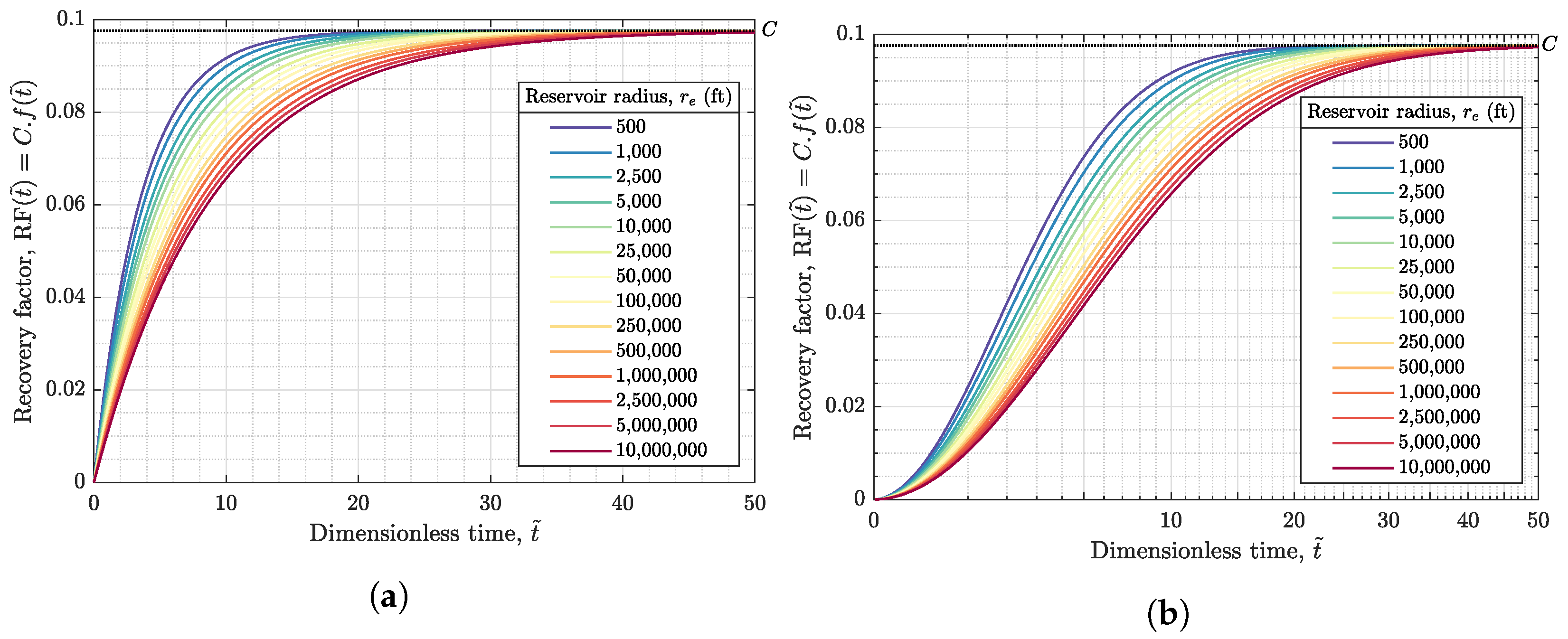
Appendix A.4. Semi-Analytical Solution of Oil Recovery Factor in Radial Flow: Bounded-Reservoir Constant-Pressure
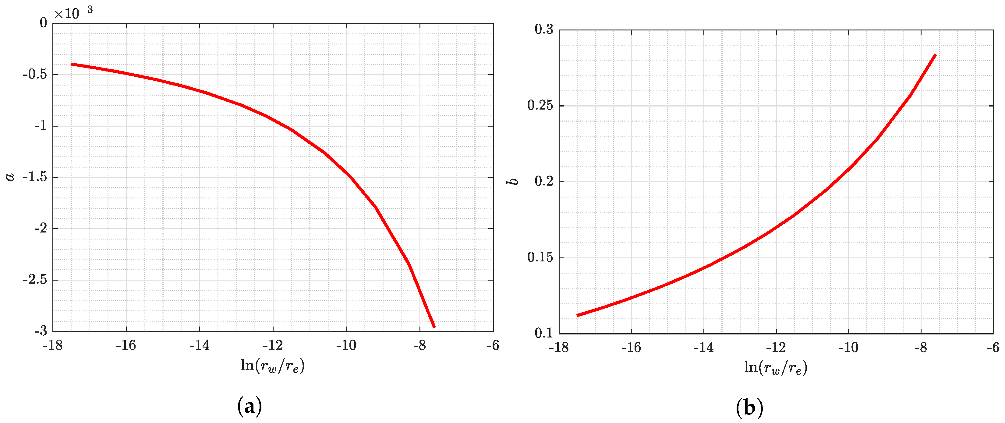
Solving the integral term in Equation (A24) is often impractical. Therefore, we try to obtain a simpler approximation of oil recovery factor. We propose a fitting function in Equation (A28) that uses two unknowns, a and b, to match each of the recovery factor curves in Figure A5:
RF ( t ˜ ) = C [ 1 e ( 1 e a t ˜ ) b / a ]
Figure A6 shows a few remarkable fits of the recovery factor, and it demonstrates that our fitting function in Equation (A28) can replicate the numerical solution for a range of reservoir radii, r e . The values of the fitting parameters a and b are summarized in Table A1.
Figure A6. Comparison between the numerical solutions and the corresponding fits from Equation (A28), for different reservoir radii, r e = (a) 500 ft, (b) 10,000 ft, (c) 250,000 ft, and (d) 10,000,000 ft.
Energies 15 00904 g0a6
Table A1. Summary of fitting parameters a and b.
r e (ft) r w / r e ln ( r w / r e ) ab
5000.00050−7.6−0.002960.284
10000.00025−8.3−0.002350.257
25000.00010−9.2−0.001790.228
50000.000050−9.9−0.001490.210
10,0000.000025−10.6−0.001260.195
25,0000.000010−11.5−0.001030.178
50,0000.0000050−12.2−0.000900.167
100,0000.0000025−12.9−0.000790.157
250,0000.0000010−13.8−0.000680.145
500,0000.00000050−14.5−0.000610.138
1,000,0000.00000025−15.2−0.000550.131
2,500,0000.00000010−16.1−0.000480.123
5,000,0000.000000050−16.8−0.000430.117
10,000,0000.000000025−17.5−0.000400.112
In Figure A7, we plot the values of a and b versus the natural logarithm of r w / r e from Table A1. Interestingly, if we take the logarithm of both axes, we obtain linear relationships shown in Figure A8. Therefore, a and b can be easily modeled as y = m x + c :
ln ( a ) = γ a [ ln ( ln ( r w / r e ) ) ] 1 a = e ( γ a [ ln ( ln ( r w r e ) ) ] 1 )
ln ( b ) = γ b [ ln ( ln ( r w / r e ) ) ] + 1 b = e ( γ b [ ln ( ln ( r w r e ) ) ] + 1 )
From Equations (A29) and (A30), the intercepts of the straight line, c, are exactly at 1 and 1. The slopes, m, are γ a 2.395 and γ b 1.115 .
Figure A7. Fitting parameters (a) a and (b) b versus ln r w / r e .
Energies 15 00904 g0a7
Figure A8. Linear relationship between (a) ln ( a ) and (b) ln ( b ) versus ln ( ln ( r w / r e ) ) .
Energies 15 00904 g0a8
Finally, the recovery factor in Equation (A26) is easy to obtain. For any reservoir radius, r e , and wellbore radius, r w , one can use the relationships in Equations (A29) and (A30) to find the parameters a and b without tedious numerical simulations.

Appendix A.5. Physical Scaling for Conventional Wells and Validations

Similar to the physical scaling approaches for unconventional hydraulically fractured wells [9,10,15,17], we can use the recovery factor in Equation (A26) as a master curve for conventional vertical wells. We first need to convert the annual oil rate, q o , ST , into the cumulative mass of oil produced m in Equation (A31):
m = ( ρ o , ST + R s ρ g , ST ) j = 1 i q o , ST ( t j ) Δ t j i = 1 i = t max
where ρ o , ST and ρ g , ST are density of oil and gas at stock-tank condition, R s is gas oil ratio, and Δ t j is one year duration.
Next, we plot both the master curve in Equation (A28) and the cumulative mass of produced oil in Equation (A31). We then scale this cumulative mass by M along the y-axis and by τ along the x-axis so that it matches the master curve. This matching process can be performed automatically using the following least square optimization problem with two unknown parameters, τ and M :
min F ( τ , M ) = m M RF ( t ˜ ) 2
For late time on production, we may expect additional exterior flow as in [11,17]. We assume that this additional flow is proportional to the square root of time with a slope K E · C :
RF E ( t ˜ ) = K E · C t ˜
The total recovery factor is the summation of interior and exterior recovery factor in Equations (A28) and (A33):
RF T ( t ˜ ) = C [ 1 e ( 1 e a t ˜ ) b / a ] + K E t ˜
The physical scaling with exterior flow has exactly the same form as before, except that now we use the master curve in Equation (A34), and there are three unknown parameters: τ , M , and K E . The corresponding optimization problem can be written as:
min F ( τ , M , K E ) = m M RF T ( t ˜ ) 2
To validate the predictive power of our physical scaling method, we built a single well reservoir model in radial coordinates using a commercial reservoir simulator, CMG. This simple model has a reservoir radius, r e , of 500 ft, initial reservoir pressure, P i , of 5000 psi, bottom-hole pressure, p w f , of 100 psi, permeability, k, of 0.1 md, and porosity, ϕ , of 0.3. Figure A9 shows pressure distribution in the reservoir model after 10 months on production and the superb match between the CMG simulation and our physical scaling method. Note that, in this case, K E = 0 because the model is limited to radial flow inside a cylindrical reservoir.
In Figure A10, we demonstrate that our physical scaling method can account for the late-time exterior flow. The matches are remarkably good with K E = 0.022 and K E = 0.035 , respectively. In addition, the external oil influx ( K E t ˜ ) in our recovery factor function may already be accounting for the unknown to us effects of waterfloods and CO2 floods in some of the Permian reservoirs. Otherwise, if reservoir-specific production data are known, these effects could be taken into account by adjusting the constant C in Equation (A27) and by the method of superposition.
Figure A9. (a) A cylindrical reservoir model using the commercial reservoir simulator, CMG; (b) Comparison between the physical scaling curve (black) and simulation result from CMG (red).
Energies 15 00904 g0a9
Figure A10. Comparison between the master curves in Equation (A34) and field data from Permian Basin: (a) K E = 0.022 and (b) K E = 0.035 .
Energies 15 00904 g0a10

References

  1. Dancy, J.R. From the Drake Well to the Santa Rita# 1: The History of the US Permian Basin: A Miracle of Technological Innovation. ONE J. 2017, 3, 1183. [Google Scholar]
  2. Tang, C.M. Permian Basin. Available online: https://www.britannica.com/place/Permian-Basin (accessed on 19 September 2021).
  3. Vertrees, C.D. Permian Basin. Available online: https://www.tshaonline.org/handbook/entries/permian-basin (accessed on 19 September 2021).
  4. Smith, T. The Permian Basin—A Brief Overview. GEOExpro 2013, 9, 1. [Google Scholar]
  5. Enverus. Permian Basin: Ultimate Guide for Permian News, Information, Facts & Statistics. Available online: https://www.enverus.com/permian-basin/ (accessed on 19 September 2021).
  6. Fed, D. Energy in the Eleventh District: Permian Basin. Available online: https://www.dallasfed.org/research/energy11/permian.aspx (accessed on 19 September 2021).
  7. EIA. Assumptions to the Annual Energy Outlook 2021: Oil and Gas Supply Module. US Energy Information Administration: Annual Energy Outlook. 2021; p. 5. Available online: https://www.eia.gov/outlooks/aeo/ (accessed on 1 December 2021).
  8. Gaswirth, S.B.; French, K.L.; Pitman, J.K.; Marra, K.R.; Mercier, T.J.; Leathers-Miller, H.M.; Schenk, C.J.; Tennyson, M.E.; Woodall, C.A.; Brownfield, M.E.; et al. Assessment of Undiscovered Continuous Oil and Gas Resources in the Wolfcamp Shale and Bone Spring Formation of the Delaware Basin, Permian Basin Province, New Mexico and Texas, 2018; US Geological Survey: Denver, CO, USA, 2018. Available online: https://pubs.er.usgs.gov/publication/fs20183073 (accessed on 1 December 2021). [CrossRef]
  9. Patzek, T.W.; Male, F.; Marder, M. From the Cover: Cozzarelli Prize Winner: Gas production in the Barnett Shale obeys a simple scaling theory. Proc. Natl. Acad. Sci. USA 2013, 110, 19731–19736. [Google Scholar] [CrossRef] [Green Version]
  10. Patzek, T.W.; Male, F.; Marder, M. A simple model of gas production from hydrofractured horizontal wells in shales. AAPG Bull. 2014, 98, 2507–2529. [Google Scholar] [CrossRef]
  11. Eftekhari, B.; Marder, M.; Patzek, T.W. Field data provide estimates of effective permeability, fracture spacing, well drainage area and incremental production in gas shales. J. Nat. Gas Sci. Eng. 2018, 56, 141–151. [Google Scholar] [CrossRef]
  12. Marder, M.; Eftekhari, B.; Patzek, T.W. Solvable Model for Dynamic Mass Transport in Disordered Geophysical Media. Phys. Rev. Lett. 2018, 120, 138302. [Google Scholar] [CrossRef] [PubMed] [Green Version]
  13. Patzek, T.W.; Saputra, W.; Kirati, W.; Marder, M. Generalized Extreme Value Statistics, Physical Scaling, and Forecasts of Gas Production in the Barnett Shale. Energy Fuels 2019, 33, 12154–12169. [Google Scholar] [CrossRef]
  14. Haider, S.; Patzek, T.W. The key physical factors that yield a good horizontal hydrofractured gas well in mudrock. Energies 2020, 13, 2348. [Google Scholar] [CrossRef]
  15. Patzek, T.W.; Saputra, W.; Kirati, W. A Simple Physics-Based Model Predicts Oil Production from Thousands of Horizontal Wells in Shales. In Proceedings of the SPE Annual Technical Conference and Exhibition, San Antonio, TX, USA, 9–11 October 2017. [Google Scholar]
  16. Saputra, W.; Kirati, W.; Patzek, T. Generalized Extreme Value Statistics, Physical Scaling and Forecasts of Oil Production in the Bakken Shale. Energies 2019, 12, 3641. [Google Scholar] [CrossRef] [Green Version]
  17. Saputra, W.; Kirati, W.; Patzek, T. Physical Scaling of Oil Production Rates and Ultimate Recovery from All Horizontal Wells in the Bakken Shale. Energies 2020, 13, 2052. [Google Scholar] [CrossRef] [Green Version]
  18. Male, F.; Islam, A.W.; Patzek, T.W.; Ikonnikova, S.; Browning, J.; Marder, M.P. Analysis of gas production from hydraulically fractured wells in the Haynesville Shale using scaling methods. J. Unconv. Oil Gas Resour. 2015, 10, 11–17. [Google Scholar] [CrossRef]
  19. Saputra, W.; Kirati, W.; Patzek, T.W. Generalized extreme value statistics, physical scaling and forecasts of gas production in the Haynesville shale. J. Nat. Gas Sci. Eng. 2021, 94, 104041. [Google Scholar] [CrossRef]
  20. Marder, M.; Chen, C.H.; Patzek, T. Simple models of the hydrofracture process. Phys. Rev. E 2015, 92, 062408. [Google Scholar] [CrossRef] [Green Version]
  21. Eftekhari, B.; Marder, M.; Patzek, T.W. Estimation of Effective Permeability, Fracture Spacing, Drainage Area, and Incremental Production from Field Data in Gas Shales with Nonnegligible Sorption. SPE Reserv. Eval. Eng. 2020, 23, 664–683. [Google Scholar] [CrossRef]
  22. Saputra, W.; Kirati, W.; Hughes, D.; Patzek, T.W. Forecast of Economic Gas production in the Marcellus. AAPG Bull. 2021. under review. [Google Scholar]
  23. Saputra, W. Physics-Guided Data-Driven Production Forecasting in Shales. Doctoral Dissertation, KAUST Research Repository. 2021. Available online: https://repository.kaust.edu.sa/handle/10754/673816 (accessed on 17 December 2021). [CrossRef]
  24. Fréchet, M. Sur la loi de probabilité de l’écart maximum. Ann. Soc. Math. Polon. 1927, 6, 93–116. [Google Scholar]
  25. Weibull, W. A statistical distribution function of wide applicability. J. Appl. Mech. 1951, 18, 293–297. [Google Scholar] [CrossRef]
  26. Gumbel, E.J. Statistical theory of extreme values and some practical applications. NBS Appl. Math. Ser. 1954, 33, 19–32. [Google Scholar]
  27. Saputra, W.; Albinali, A.A. Validation of the Generalized Scaling Curve Method for EUR Prediction in Fractured Shale Oil Wells. In Proceedings of the SPE Kingdom of Saudi Arabia Annual Technical Symposium and Exhibition, Dammam, Saudi Arabia, 23–26 April 2018. [Google Scholar]
  28. Arps, J. Analysis of Decline Curves. Trans. AIME 1945, 160, 228–247. [Google Scholar] [CrossRef]
  29. Saputra, W.; Kirati, W.; Patzek, T.W. Forecast of economic tight oil and gas production in Permian Basin. AAPG Bull. 2021. submitted. [Google Scholar] [CrossRef]
  30. Boltzmann, L. Zur Integration der Diffusionsgleichung bei variabeln Diffusionscoefficienten. Annalen der Physik 1894, 289, 959–964. [Google Scholar] [CrossRef] [Green Version]
  31. Zimmerman, R.W. Imperial College Lectures in Petroleum Engineering, The-Volume 5: Fluid Flow in Porous Media; World Scientific: Singapore, 2018; pp. 23–122. [Google Scholar]
  32. Muskat, M. The Flow of Compressible Fluids Through Porous Media and Some Problems in Heat Conduction. Physics 1934, 5, 71–94. [Google Scholar] [CrossRef]
  33. Everdingen, A.V.; Hurst, W. The Application of the Laplace Transformation to Flow Problems in Reservoirs. J. Pet. Technol. 1949, 1, 305–324. [Google Scholar] [CrossRef]
  34. Ehlig-Economides, C.A. Well Test Analysis for Wells Produced at a Constant Pressure. Ph.D. Thesis, Stanford University, Stanford, CA, USA, 1979. [Google Scholar]
  35. Darcy, H. Les Fontaines Publiques de la ville de Dijon: Exposition et Application; Victor Dalmont: Paris, France, 1856. [Google Scholar]
  36. Hubbert, M.K. Darcy’s law and the field equations of the flow of underground fluids. Trans. AIME 1956, 207, 222. [Google Scholar] [CrossRef]
Figure 1. (a) Annual oil rate in kbbl/yr and (b) Cumulative oil in kbbl from all 484,759 vertical wells in the Permian Basin.
Energies 15 00904 g001
Figure 2. The map of all 484,759 vertical wells in the Permian Basin, colored by completion date.
Energies 15 00904 g002
Figure 3. The map of all 484,759 vertical wells in the Permian Basin, colored by four different reservoir ages.
Energies 15 00904 g003
Figure 4. The map of all 484,759 vertical wells in the Permian Basin, colored by three classes of maximum daily oil rate.
Energies 15 00904 g004
Figure 5. (a) Number of active wells and (b) total field–daily oil rate colored by sub-play.
Energies 15 00904 g005
Figure 6. (a) Number of active wells and (b) total field–daily oil rate colored by reservoir age.
Energies 15 00904 g006
Figure 7. Procedure of arriving at a historical well prototype using GEV statistics. (Example: Midland Basin—Leonardian [2000–2009]). Each row shows different sampling of annual production after the first, second, …, n-th year on production. The first column is the probability density function (PDF) of annual production fitted with lognormal distribution (blue) and GEV distribution (red). The corresponding ξ , μ , and σ are the fitting parameters for the GEV distribution. The second column shows the maximum likelihood estimate, 95% confidence interval (CI) for μ and σ . The third column displays the cumulative distribution function (CDF), including the lower bound, P 90 , median, P 50 , and upper bound, P 10 , with its confidence interval. The last column shows the resulting historical well prototype, which is constructed by connecting the expected GEV values (means) of each row.
Energies 15 00904 g007
Figure 8. Historical well prototypes (solid lines) and the corresponding physical scaling forecasts (dashed lines) for the 192 well cohorts. The columns represent the four reservoir ages, while the rows denote the eight different completion date intervals. The six different sub-plays are encoded with different colors. The horizontal bar charts show the percentage of each subset sub-play from the total n sample of each reservoir-age × completion-date combination. In addition, the small square at the right boundary of each graph shows the average ultimate recovery for the six sub-play scenarios.
Energies 15 00904 g008
Figure 9. Distribution of fitting parameters for physical scaling: (a) τ , GEV mean = 2.37 years and (b) M , GEV mean = 106.37 ktons.
Energies 15 00904 g009
Figure 10. Survival probability plot for Permian region: (a) Central Basin—Leonardonian and (b) Midland Basin—Wolfcampian. The fitting function is y ( t ) = ( 1 + β ) ( e t β β ) .
Energies 15 00904 g010
Figure 11. (a) Total field rate, (b) Total field cumulative forecasts from existing 484,759 wells in the Permian Basin.
Energies 15 00904 g011
Figure 12. Evolution of completion depth in the Permian Basin. The upper bound, P 10 , the expected value, P 50 , and the lower bound, P 90 are all calculated with GEV statistics.
Energies 15 00904 g012
Table 1. Summary of four reservoir ages and list of reservoir names included. The cross-ticked boxes indicate the existence of each reservoir layer in six different areas (sub-plays).
NoReservoir AgeTime (m.y.)Reservoir NameAreal Extent
Delaware BasinNorthwest ShelfCentral BasinEastern ShelfMidland Basin
1Guadalupian251Bell Canyon
Delaware
Capitan
Tansill
Yates
Seven Rivers
Queen
Grayburg
San Andres
Holt
Brushy Canyon
2Leonardian275Bone Spring
Spraberry
Dean
Glorieta
Paddock
Blinebry
Clear Fork
Tubb
Drinkard
Yeso
Abo
3Wolfcampian290Wolfcamp
4Pre-Permian302–495Pennsylvanian
Cisco
Canyon
Strawn
Atoka
Morrow
Barnett
Mississippian
Devonian
Silurian
Fusselman
Ordovician
Montoya
Simpson
Ellenburger
Table 2. Design of 192 well cohorts = 4 reservoir ages × 6 sub-plays × 8 completion dates.
4 Reservoir Ages6 Sub-Plays8 Completion Dates
GuadalupianCentral Basin1930–1949
LeonardianMidland Basin1950–1959
WolfcampianDelaware Basin1960–1969
Pre-PermianNorthwest Shelf1970–1979
Eastern Shelf1980–1989
Others1990–1999
2000–2009
2010–2021
Table 3. Summary of maximum survival times, t surv , in years for the Permian regions.
GuadalupianLeonardianWolfcampianPre-PermianMean
Delaware Basin7047352043
Northwest Shelf9578473163
Central Basin7887445767
Eastern Shelf5091483957
Midland Basin9477405065
Others4527101925
Mean7268373653
Publisher’s Note: MDPI stays neutral with regard to jurisdictional claims in published maps and institutional affiliations.

