Article

Wind Speed Forecasts of a Mesoscale Ensemble for Large-Scale Wind Farms in Northern China: Downscaling Effect of Global Model Forecasts

1
Key Laboratory for Aerosol-Cloud-Precipition of China Meteorological Administration, Nanjing University of Information Science and Technology, Nanjing 210044, China
2
Precision Regional Earth Modeling and Information Center, Nanjing University of Information Science and Technology, Nanjing 210044, China
3
National Center for Atmospheric Research, Boulder, CO 80307, USA
4
Inner-Mongolia Meteorological Bureau, Huhhot 010051, China
5
Electric Power Dispatch Center, Jibei Electric Power Company, Beijing 100054, China
*
Authors to whom correspondence should be addressed.
Energies 2022, 15(3), 896; https://doi.org/10.3390/en15030896
Submission received: 7 December 2021 / Revised: 14 January 2022 / Accepted: 25 January 2022 / Published: 26 January 2022

Abstract

:
To facilitate wind power integration for the electric power grid operated by the Inner Mongolia Electric Power Corporation—a major electric power grid in China—a high-resolution (of 2.7 km grid intervals) mesoscale ensemble prediction system was developed that forecasts winds for 130 wind farms in the Inner Mongolia Autonomous Region. The ensemble system contains 39 forecasting members that are divided into 3 groups; each group is composed of the NCAR (National Center for Atmospheric Research) real-time four-dimensional data assimilation and forecasting model (RTFDDA) with 13 physical perturbation members, but driven by the forecasts of the GFS (Global Forecast System), GEM (Global Environmental Multiscale Model), and GEOS (Goddard Earth Observing System), respectively. The hub-height wind predictions of these three sub-ensemble groups at selected wind turbines across the region were verified against the hub-height wind measurements. The forecast performance and variations with lead time, wind regimes, and diurnal and regional changes were analyzed. The results show that the GFS group outperformed the other two groups with respect to correlation coefficient and mean absolute error. The GFS group had the most accurate forecasts in ~59% of sites, while the GEOS and GEM groups only performed the best on 34% and 2% of occasions, respectively. The wind forecasts were most accurate for wind speeds ranging from 3 to 12 m/s, but with an overestimation for low speeds and an underestimation for high speeds. The GEOS-driven members obtained the least bias error among the three groups. All members performed rather accurately in daytime, but evidently overestimated the winds during nighttime. The GFS group possessed the fewest diurnal errors, and the bias of the GEM group grew significantly during nighttime. The wind speed forecast errors of all three ensemble members increased with the forecast lead time, with the average absolute error increasing by ~0.3 m/s per day during the first 72 h of forecasts.

1. Introduction

Wind energy, with its vast availability, cleanliness, and renewability, is growing rapidly in the energy share, and plays an increasingly important role in the electric energy sector [1]. However, the intermittent and volatile nature of wind speeds poses a great challenge to the grid-connected transmission of wind power output, threatening the security of the grid system and sometimes leading to massive wind abandonment [2]. Reliable wind power forecasting is urgently needed for timely and accurate dispatch of power resources [3,4]. Wind speed forecasting methods include statistical approaches, machine learning methods [5,6,7,8,9,10,11], and numerical weather prediction [12]. There have been many works on wind prediction reported in the past two decades, especially over the last few years. However, most of these works are on the refinement of statistical and AI approaches [13,14,15,16,17,18]; there have been very few studies examining and analyzing the errors of numerical weather models. As a matter of fact, for wind forecasts beyond ~1 h, numerical weather prediction models become essential and fundamental. Improving the performance and capability of numerical weather prediction models and machine learning post-processing for wind farm weather prediction is therefore critical.
The performance of numerical weather models relies greatly on model resolutions [19] and regional climates [20], topography [21], underlying land-surface and soil properties [20], weather measurements [22] and data assimilation schemes for model initiation [23], as well as the lateral boundary conditions for limited-area models [24]. For these reasons, many studies and energy forecasting firms use an ensemble of global and regional NWP outputs to reduce forecast errors [25,26].
There are three main error sources in numerical weather forecasting: uncertainties in initial values [27], approximation of the dynamical and physical models [28], and the intrinsic unpredictability of atmospheric motions [29]. Ensemble numerical weather prediction methods [30,31] have been used to improve the accuracy and reliability of weather forecasts through probabilistic forecasts. Probabilistic forecasts and uncertainty quantification are beginning to take the place of single numerical forecasts in the wind energy industry. An ensemble forecast system can simulate the impact of the uncertainties of initial and boundary conditions derived from different global model forecasts, atmospheric physical parameterization schemes, and data assimilation modules. Perturbation members of a mesoscale ensemble forecast system include sub-grid energy stochastic perturbation members, physical parameterization perturbation members, initial and boundary value perturbation members, and some others. Analyzing the error characteristics of ensemble forecast members is important for exploring the value of ensemble forecast outputs and improving the ensemble forecast system.
With respect to model forecast verification, several researchers have explored the effects of model physical processes on wind speed forecasting [32,33,34,35,36]. Different physical parameterization schemes often present different forecast capabilities under different meteorological conditions or regimes [24,37,38], different geographical regions [39,40,41,42], and/or different topographic environments [43]. In responding to atmospheric long- and short-wave radiative forcing, model forecast errors often exhibit diurnal and seasonal variations [44,45,46,47]. Some other researchers focused on revising model forecast results through post-processing by using statistical and machine learning methods [48]. However, the errors of the model initial and boundary conditions derived from different global model background fields are often large [49,50], but very little attention has been paid to this issue [51]. In fact, we could not find any report investigating the impact of model initial and boundary conditions of the wind farm wind forecasting based on a 2–4 km grid high-resolution ensemble numerical weather prediction model.
The wind energy density in the Inner Mongolia Autonomous Region, China, is outstanding—over 400 W/m2 in some regions [52]. In 2019, wind power generation in Inner Mongolia was 66.6 billion kWh, accounting for ~16.4% of China’s total wind power generation in the same period (China National Energy Administration). In response to the demand for wind power integration in Inner Mongolia, the Inner Mongolia Electric Power Company (IMEPC) has developed a mesoscale ensemble numerical weather prediction system that is composed of 39 perturbed WRF (Weather Research and Forecasting) forecast members. The system is constructed with multiple global models of forcing, multiple physical parameterization schemes, and stochastic kinetic energy perturbations. The 39 forecast members contain three subgroups of 13 physical perturbation members, driven by the forecasts of the GFS (Global Forecast System), GEM (Global Environmental Multiscale Model), and GEOS (Goddard Earth Observing System), respectively.
This paper evaluates the output of the IMEPC mesoscale ensemble prediction system, focusing on its hub-height wind prediction for the wind farms distributed across the Inner Mongolia Autonomous Region during the spring of 2020. The model performance of three sub-ensemble groups driven by the forecasts of the GFS, GEOS, and GEM global models was studied, and the variations in the forecast errors with forecast lead time, wind speed regimes, diurnal forcing, and regional changes were analyzed. The findings of this study provide guidance for the proper use of the ensemble prediction system at the wind farms, and for the development of model forecast post-processing capabilities by the IMEPC. Our results also support modelers to improve the ensemble model system by adjusting the ensemble members according to the error properties of the ensemble members driven by different global model forecasts.
The remainder of this paper is organized as follows: Section 2 describes the observations in the study area and the setup of the ensemble forecast system used for the numerical experiments. Section 3 presents the results of the wind speed forecast error analysis. Section 4 presents the conclusions from these analyses. Finally, Section 5 discusses the limitations of the present work, and describes the outlook for the future.

2. Data and Meteorology

2.1. Ensemble Numerical Weather Prediction System

The IMEPC’s WRF-based ensemble weather forecasting system produces wind power forecasts over 100 wind farms distributed across the Inner Mongolia Autonomous Region. This system was jointly developed by the Inner Mongolia Meteorological Bureau, the US National Center for Atmospheric Research (NCAR), and Nanjing University of Information Science and Technology (NUIST); it started real-time operational forecasting in late 2019. The system uses the forecasts of the GEOS (USA), GEM (Canada), and GFS (USA) to derive the initial and boundary conditions to drive the WRF forecast members. The system is configured with 10 physical parameterization schemes, including 9 boundary layer schemes and 1 radiation scheme, and 3 stochastic kinetic energy backward feedback dynamical perturbation (SKEP) schemes, making up the 13 perturbation members that are driven by initial and boundary conditions derived from the global model forecasts of the GFS, GEM, and GEOS, respectively. The system constitutes a total of 39 ensemble forecast members.
The details of the 13 WRF members are listed in Table 1. Each member runs with the WRF real-time four-dimensional data assimilation system (WRF-RTFDDA) [23,53,54,55]. The operational ensemble forecast system runs with 3-hour data assimilation and forecast cycles, and each cycle produces 72-hour forecasts at a temporal resolution of 15 min. The system assimilates the observations of the hub-height wind speed (the wind turbine wind speed) and meteorological tower weather observations of the wind farms in the region, along with various conventional weather observations [56,57,58].
The ensemble model contains three forecast domains (Figure 1). Domain 2 and Domain 3 cover the central and western plateau regions of the Inner Mongolia Autonomous Region (40~45° N, 105~120° E), at 2.7 km grid intervals. Domains 2 and 3 are embedded in a coarser grid domain (Domain 1) with a grid size of 13.5 km. Most of the wind farms studied in this paper are located in Domains 2 and 3, featuring complex terrain including stratified high plains, stony hills, terraces, foothills, and inter-hill lowlands. The wind farms are mostly built around four major mountain ranges, including Langshan Mountain (LS), Seertengshan Mountain (SRTS), Ural Mountain (ULS), and Daqingshan Mountain (DQS), along with fan sites located near the Yinshan Mountains (YS), a low plain area to the south of the Hetao Plain (HTPY), and a high plain area near the Xilin Gol League (XLGL) (Figure 1b).

2.2. The Observations and Forecasts

Verification statistics of the ensemble forecasts were calculated based on 411 representative wind turbine sites selected from 130 wind farms, with 1–4 wind turbine sites per wind farm, depending on the wind farm’s size. The wind turbine sites are mainly distributed in central Inner Mongolia (Figure 1b). The analysis period was from 1 March to 15 April 2020. Wind speeds at the hub height of the wind turbines, ~50–80 m high from the ground, were retrieved from the SCADA (Supervisory Control and Data Acquisition System) of the wind turbines and averaged to 15-minute windows. To maintain the data continuity, for periods with less than an hour of missing data, a linear interpolation was used to fill in the gaps. For computing the verification statistics, forecasts of the ensemble numerical weather prediction were interpolated to the location and hub height of the selected turbines through a bilinear interpolation method, forming observation and forecast-matched pairs for direct comparison. With 411 wind turbines, 45 days, 72 h of forecasts per day at 15 min intervals, and 39 ensemble members, there were a total of 207,735,840 data samples processed in the verification computation.
To analyze the regional differences in the model forecasts, the wind farms were divided into seven sub-areas according to the distribution of wind farm clusters and topographic characteristics. These areas are marked in the cyan boxes in Figure 2. The wind farm sites in Area 1 are located on the northern slope of Langshan Mountain. The sites in Area 2 are mostly concentrated between Langshan Mountain and Seertengshan Mountain. Area 3 is over the southern part of the Loop Plain to the north of the mountain. Area 4 is between Seertengshan Mountain and Ural Mountain, and some of the turbine sites are close to the local mountain peaks. Area 5 is in the eastern part of Ural Mountain, with higher elevation. Area 6 is located in the relatively more complex area of Daqingshan Mountain to the west of Ural Mountain, with lower elevation, and the turbine sites are more dispersed. Finally, Area 7 is characterized by a high plain area with a flattering topography near the Xilin Gol League. The numbers of stations in these sub-areas are 22, 61, 13, 131, 72, 72, and 40, respectively.

2.3. Evaluation Metrics

The statistical verification of the ensemble forecasts includes calculation of systematic error (BIAS), mean absolute error (MAE), and correlation coefficient (CC) for all selected wind turbine sites and the wind turbine sites in each sub-area. The ensemble wind speed forecast performance is assessed by examining both individual metrics and their combinations. The three statistical variables are calculated based on the hub-height observed (Xo) and forecast (Xf) 15-minute mean wind speed pairs.

3. Statistical Verification Results

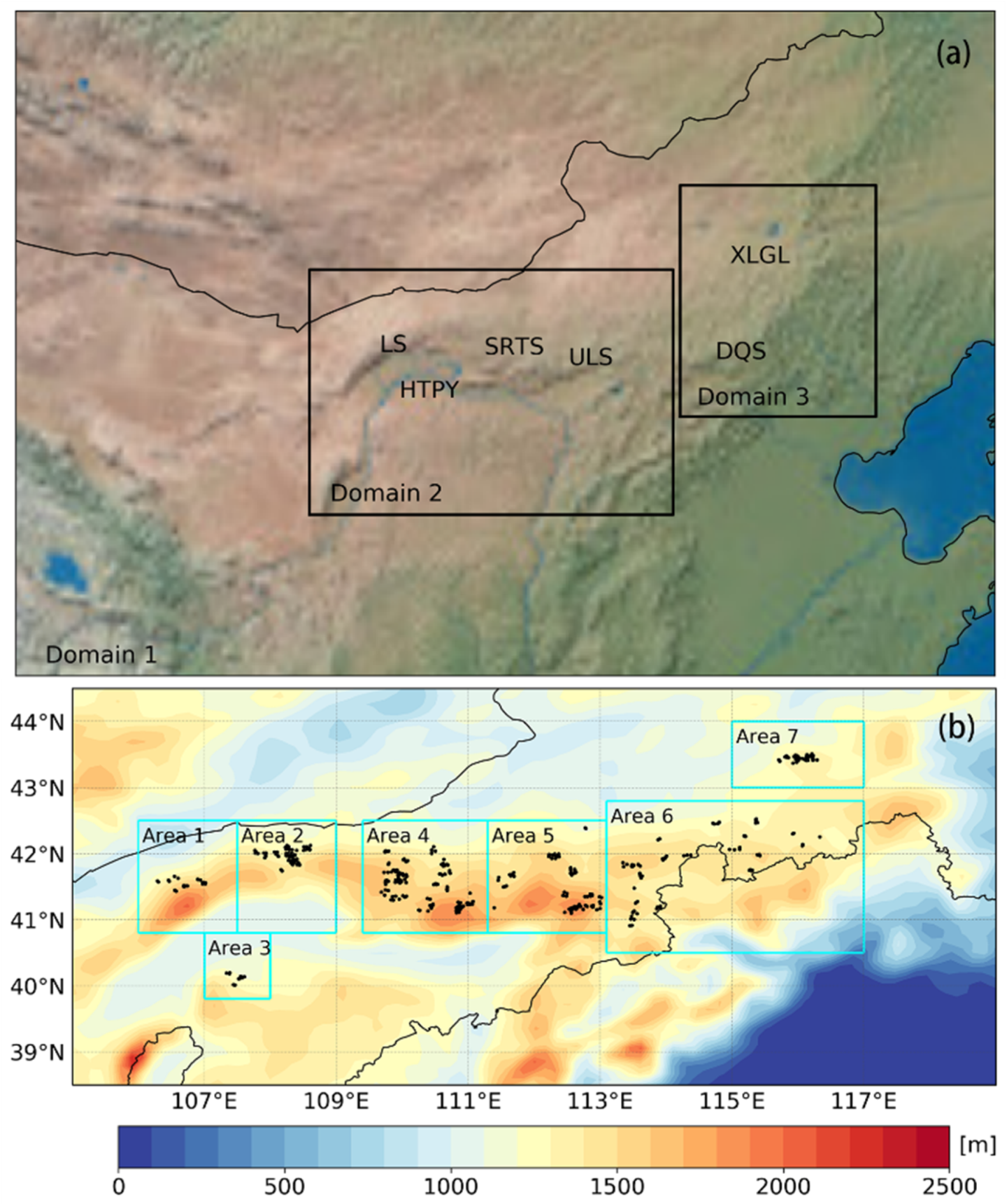
3.1. Characteristics of the Winds in the Region

Figure 2 shows the diurnal variation in wind speed observations averaged at all wind turbine sites over the study area, as well as those in the seven sub-areas given in Figure 1. The wind speed over the whole region (Figure 2) exhibits evident diurnal variations, with errors gradually increasing during daytime (from 00:00 to 09:00 UTC, i.e., 08:00–17:00 LST). The median wind speed maximizes between 09:00 UTC and 10:00 UTC (~6.8 m/s), and then starts to decrease in the nighttime. The 25 and 75% sub-quartile wind speeds are 4.2 and 8.2 m/s, respectively; ~5% of the wind speeds are greater than 12 m/s, and ~5% of the wind speeds are less than 2 m/s.
Although the median wind speeds in all seven sub-areas are close (~6 m/s), the diurnal variations in the wind speeds in these regions are quite large. Area 1 possesses a high peak wind speed at 02:00 UTC and 15:00 UTC, and is also prone to greater wind speeds during the day–night transition. The median wind speed in Area 2 tends to slowly increase during daytime, with two local maxima at 03:00 UTC and 09:00 UTC, respectively. The wind speed in Area 3 is higher at night, with a peak median wind speed at 18:00 UTC.
Wind farms in Areas 4, 5, and 6 are in complex mountainous terrain, where winds increase until 09:00–10:00 UTC during the daytime, and show a decreasing trend at night. Finally, Area 7 is in a high plain region, and the diurnal variation in its wind speed is relatively flat, with a small peak in the afternoon, a small trough in the evening, and then a gradual rebound at night.

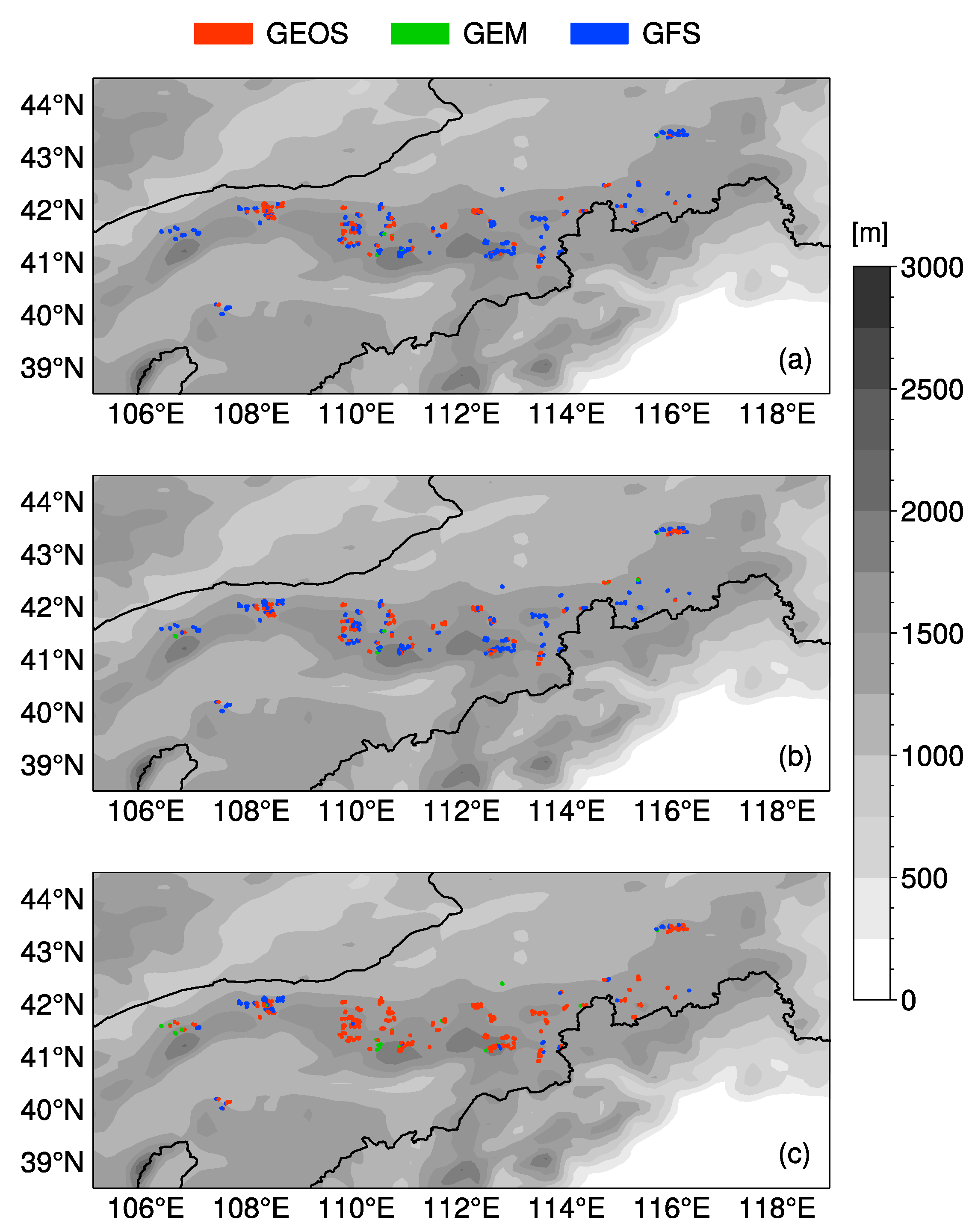
3.2. Overall Performance of the Wind Forecasts

To compare the forecasts of the ensemble members driven by the initial and boundary conditions derived from the three global model forecasts (GFS, GEOS, and GEM), we first calculated the error metrics of each ensemble member, and then averaged the errors of the 13 members within each subgroup. The average error for each sub-group is computed as follows:
x m = 1 13 i = 1 13 x i
where x i (m/s) represents the error metrics of the forecast of the ith ensemble member. With verification done for 0–24 h forecasts for the 45 days for all 411 wind turbines, the total number of data samples used in computing the statistical verification in each cell of the Table 2 was 23,081,760.
The overall performance of the three groups of global model forecast members, along with the CC, BIAS, and MAE of the 0–24-hour wind turbine hub-height wind forecasts of all members of the three groups, are calculated and shown in the ‘mean’ column in Table 2. The CC and MAE of the wind forecasts of the GFS group are better than those of the GEOS group, and both are better than those of the GEM group. In contrast, the BIAS in the GEOS group is smaller than that in the GFS group. The GEM group has the worst scores for all three metrics. The minimum, maximum, and median of correlation coefficients, mean errors, and mean absolute errors of 13 member predictions (13 outcomes for each background field) versus observations are shown in the ‘min’, ‘max’, and ‘median’ columns, respectively, in Table 2. Ensemble average forecasts outperformed the best members. Overall, the GFS group was better than GEOS, and GEM was the worst, which is statistically significant (with all at a confidence level above 98%).
To assess the overall performance of the members driven by the three global model forecasts, the statistical metrics of the three group ensemble forecasts were ranked from the best to the worst for each wind turbine site. The number of stations that performed the best and worst by each ensemble group was counted, as shown in Table 3, along with their proportion to the total turbine sites. The performance of the three ensemble forecast groups varies with the geographic setting of the turbines, as well as the local regional weather and climate characteristics. The statistical verification metrics were calculated separately for each site.
Among the three forecast groups, the GFS groups performed the best at ~59–64% of the total sites in terms of CC and MAE, the GEOS group achieved ~34–37%, and the GEM group performed the best for the remaining ~2%. Conversely, from the perspective of the worst performance of the forecasts, the GEM group underperformed at ~77–86% of sites, the GEOS group at ~11–20%, and the GFS group at only ~2–3%. It is interesting to point out that the GEOS group performed the best (~77% of sites) in terms of BIAS, and had relatively more cases with larger positive and negative deviations.
Figure 3 shows the distribution of the turbine sites colored for the predominant best performing ensemble group in terms of the mean CC, BIAS, and MAE among the three ensemble forecast member groups driven by the GFS, GEOS, and GEM global model forecasts. In general, the sites that achieved the best CC and the best MAE coincide. Nevertheless, for BIAS, the GEOS group performed the best at the most turbine sites.

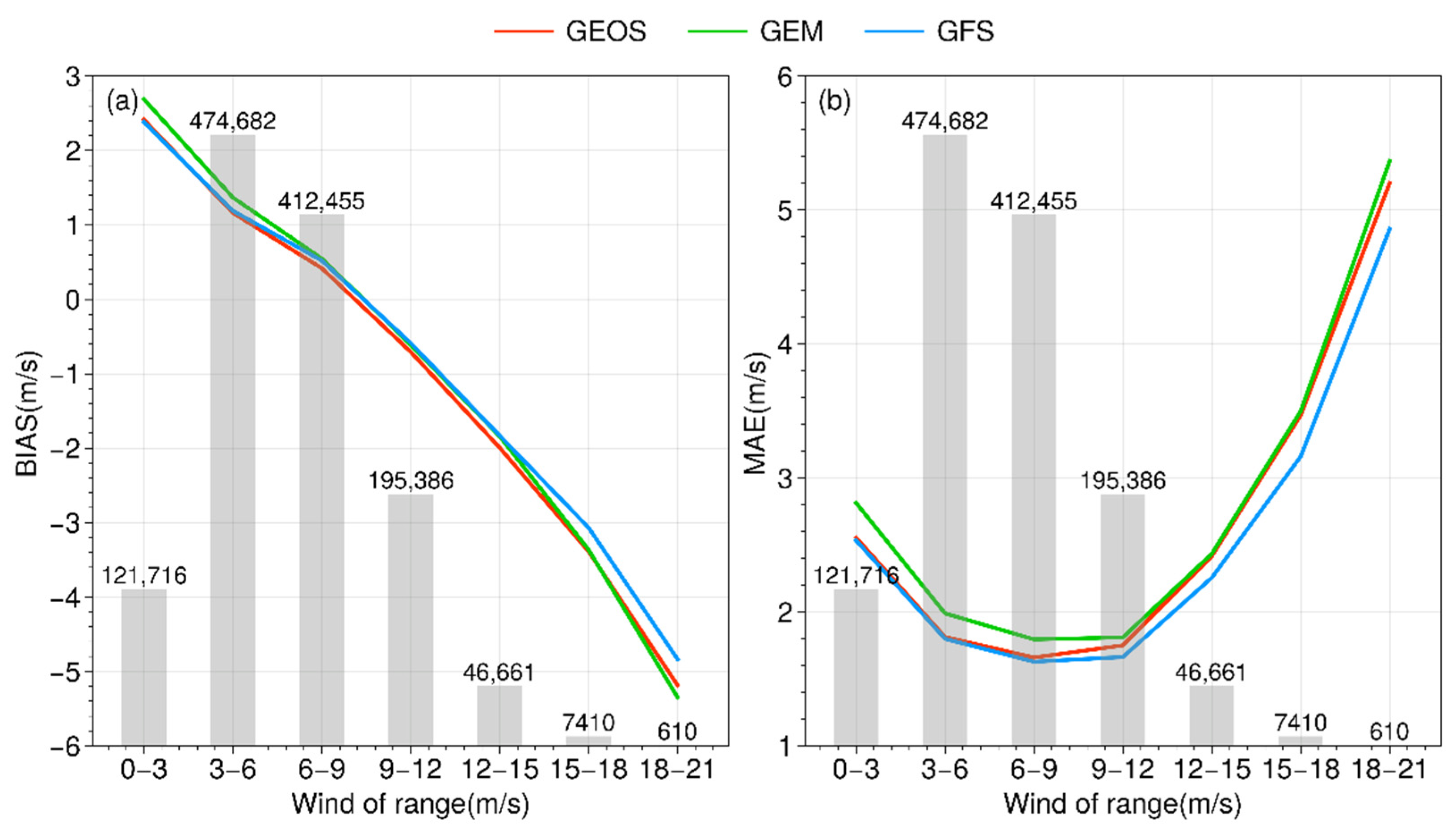
3.3. Variations of Forecast Errors with Wind Regimes

Wind power generation is proportional to the cubic wind speed [68]. Therefore, it is important to evaluate the model performance in different ranges of wind speeds. Herein, the wind speed is divided into bins of 3 m/s from 0 to 21 m/s, and the forecast errors for each wind speed bin are computed and shown in Figure 4.
The winds in the region are mostly 3–12 m/s (Figure 4). The wind forecast bias of all three groups is similar. The wind forecast bias is negatively correlated with the observed wind speeds, with a nearly linear relationship. For the weak wind conditions of 0–3 m/s, the wind speed is overestimated by 2 m/s. In the bin of 3–9 m/s, the bias gradually decreases to 0, and then the negative bias gradually increases with the wind speed. For winds over 15 m/s, the negative bias reaches 4–5 m/s. The MAE of the wind forecast of the three groups is around 2 m/s in the wind speed range of 3–12 m/s. The overestimation of wind speed in the low-wind-speed range (0–3 m/s) and the underestimation of wind speed in the high-wind-speed range lead to larger MAE for the weak and strong wind ranges.
For the winds in the range of 0–6 m/s, the forecast errors of the GFS and GEOS groups are basically the same, and both are better than the GEM group. For strong winds over 12 m/s, the forecast errors of the GEOS and GEM groups are very similar, and worse than the GFS group. The overestimation of wind speeds in the low-wind-speed range and the underestimation of wind speeds in the high-wind-speed range are smaller for the GFS group than for the other two groups.

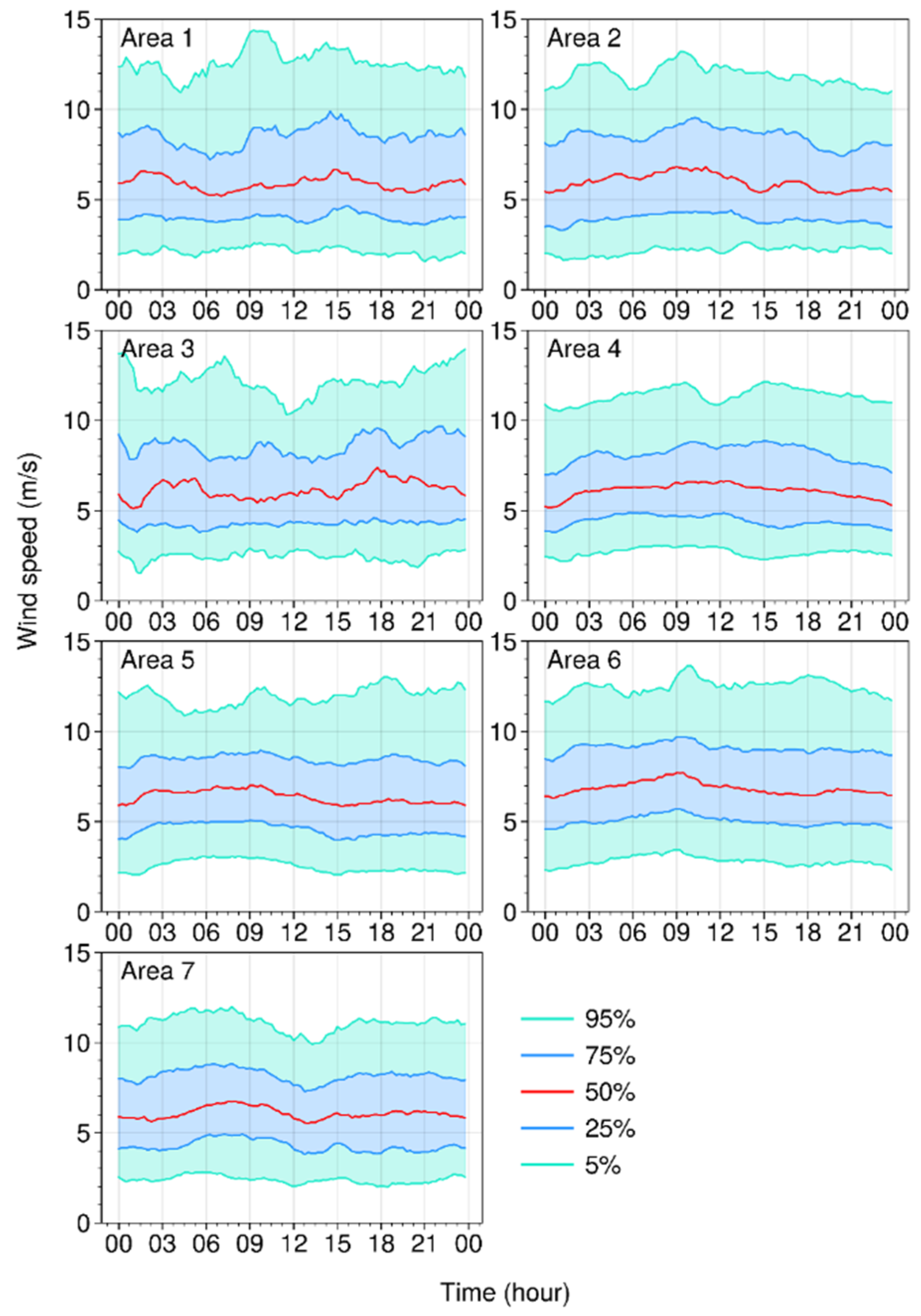
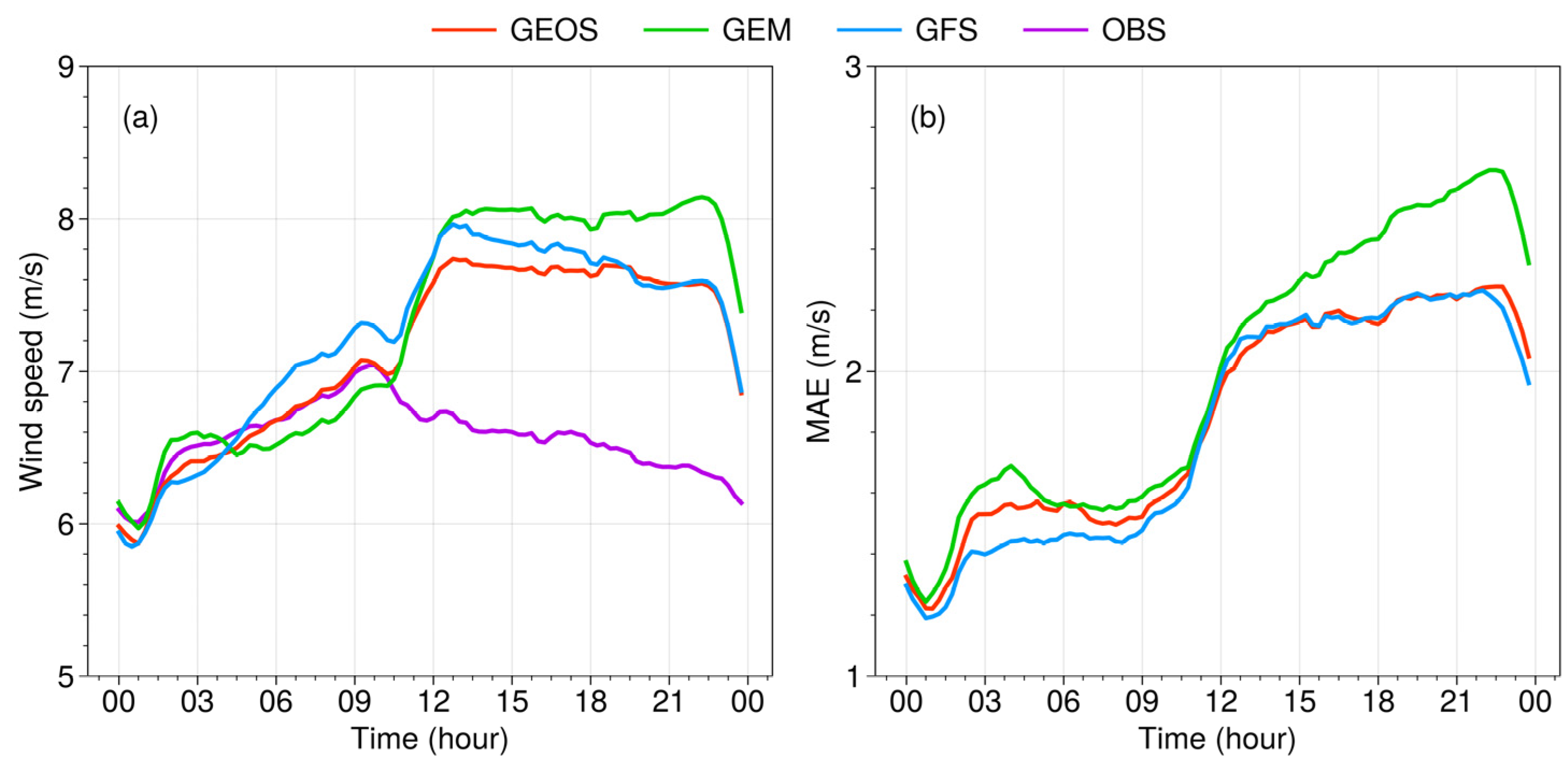
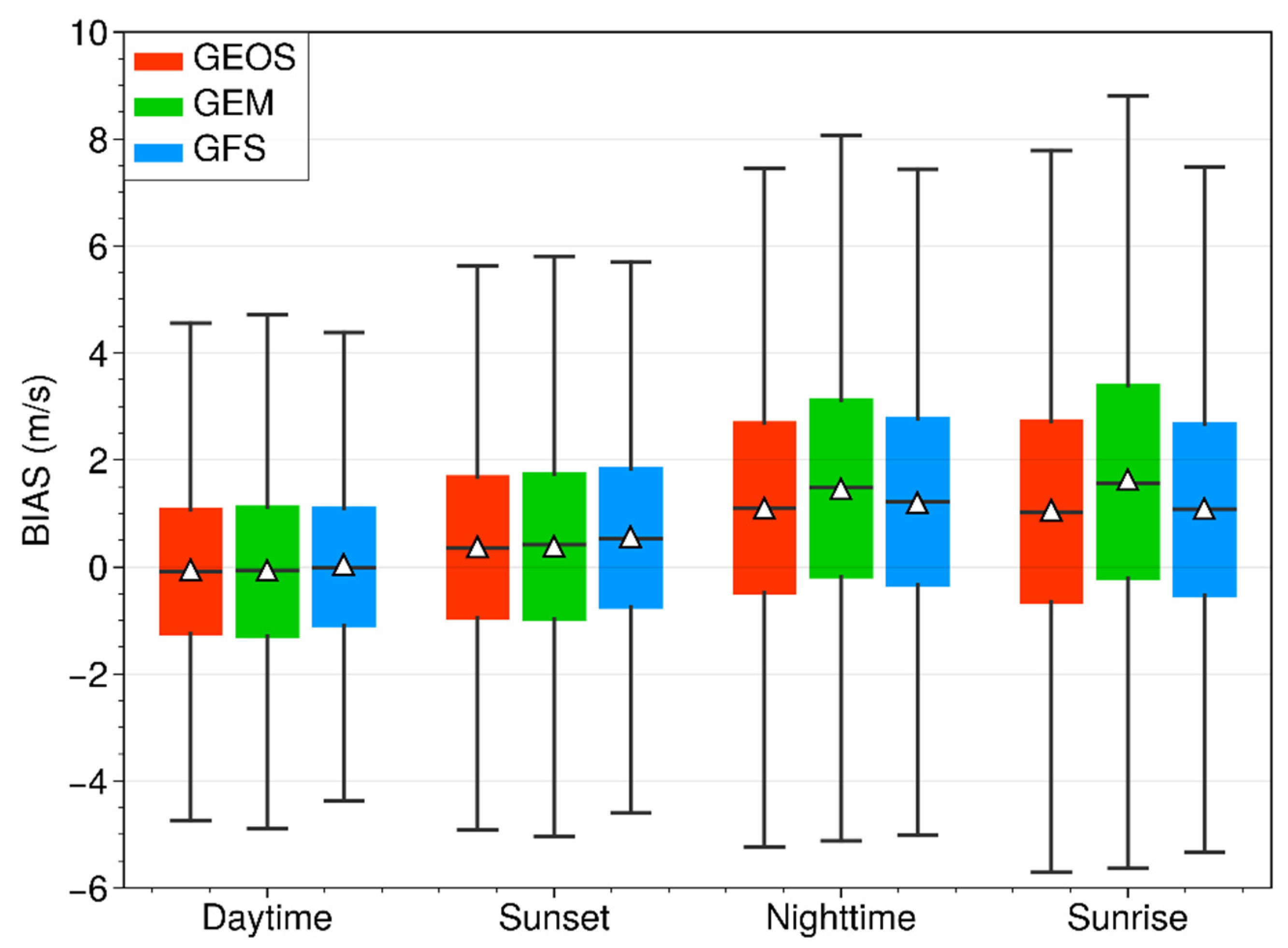
3.4. Diurnal Variation in Wind Forecast Errors

Figure 5 presents the diurnal variation of the mean observations, and the forecasts and MAE of the wind speed for the ensemble groups driven by the GFS, GEOS, and GEM forecasts. During daytime (00:00–09:00 UTC), the mean wind speed increases from 6 m/s to 7 m/s from morning to evening. Overall, the bias of the wind forecasts of all three groups is small. The GEOS group shows a bias close to zero, the GEM group has a weak negative deviation, and the GFS group has a bias that gradually increases from a negative deviation of ~0.1 m/s to a positive deviation of 0.2 m/s.
At ~11:00 UTC, the wind forecasts of all three ensemble groups experience a sharp increase toward a positive deviation. Within half an hour, the bias of the wind forecasts of the GEOS, GFS, and GEM groups increases to ~0.9, 1.1, and 1.3 m/s, respectively. Subsequently, at night, the mean wind speed gradually weakens and the mean bias of the wind speed forecasting of the GFS group remains roughly unchanged, but the mean deviation in the GEOS and GEM groups continues to increase. By 23:00 UTC, the positive wind forecast biases of all three groups decrease rapidly as the boundary layer starts to grow after sunrise.
The GEM ensemble group possesses the largest MAE of the wind forecasts during daytime, followed by the GEOS group, while the MAE of the GFS group is the lowest. After a brief increase, MAE stabilizes at ~1.5 m/s between 03:00 and 11:00 UTC. After sunset (11:00–13:00 UTC), the MAE of all three groups increases to ~2.2 m/s. After nightfall, the MAE of the wind speed forecast of the GEM group continues to increase significantly, to 2.7 m/s, while that of the GEOS and GFS groups only increases to 2.3 m/s. Finally, after sunrise at 22:00 UTC, the MAE of all three groups decreases rapidly. Overall, the MAE of the GFS group was smaller than that of the other two groups, and the MAE of the GEM group was the largest for both nighttime and daytime. The MAE of the GEOS group during nighttime is similar to that of the GFS group.
To further compare the distribution of the wind forecast errors of the three ensemble groups and their diurnal variations, the forecast deviations of each ensemble member were analyzed for four day-periods: daytime (00:00–10:00 UTC), sunset (10:00–12:00 UTC), nighttime (12:00–22:00 UTC), and sunrise (22:00–00:00 UTC); the results are summarized in Figure 6.
The error distributions of the wind forecasts of all three groups are quite wide. The forecast members of the GFS group have relatively smaller variance (i.e., smaller dispersion) than the other two groups. In contrast, the forecast members of the GEM group have relatively larger variance and median bias. During the daytime and sunset periods, the error distributions of the three ensemble groups are relatively similar, and the numbers of samples with positive and negative deviations are close. However, during the night and sunrise phases, most of the model forecasts in all groups overestimate the wind speed, and the positive deviations of the GEM group are significantly larger than those of the GFS and GEOS groups.

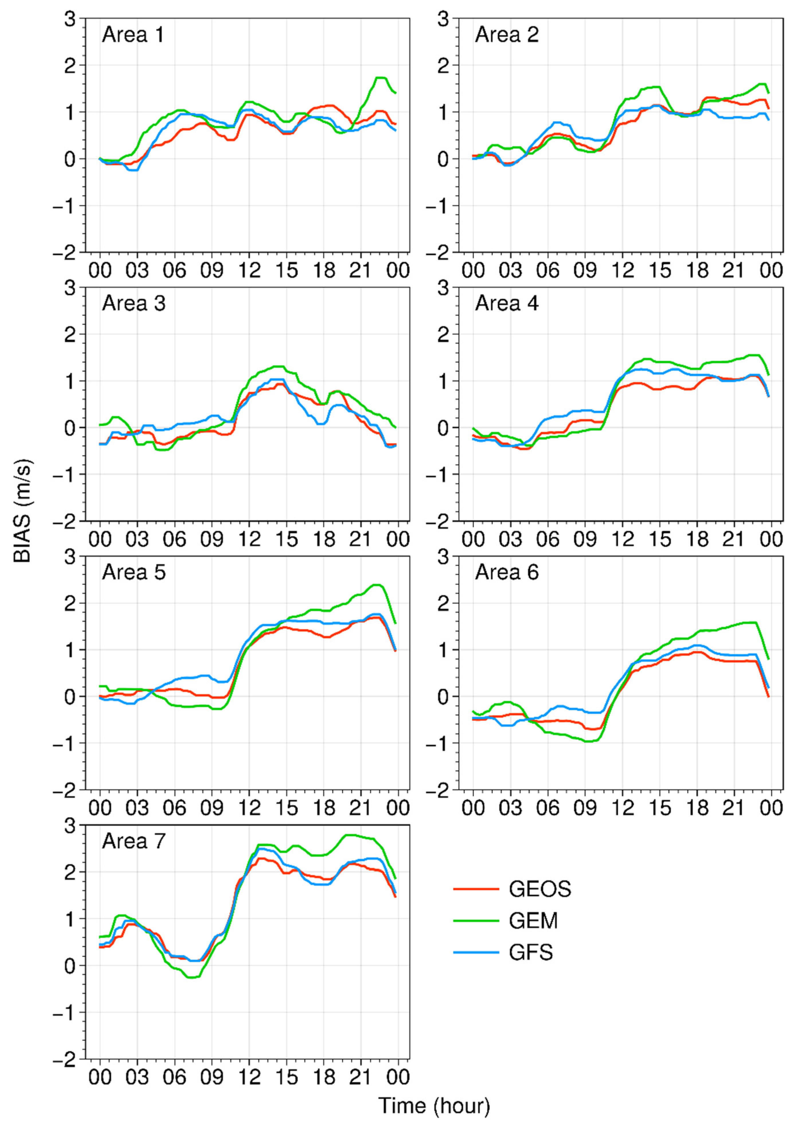
3.5. Forecast Errors in Seven Regions

The previous analysis indicates that the ensemble members driven by the three global model forecasts perform differently at different sites (Figure 3). To further investigate the regional differences in these ensemble groups, the wind farms in the study area were divided into seven sub-areas, according to geographical location, from west to east (see Figure 1). As shown in Figure 1, the wind farms are mainly built along the narrow mountain ridges that span the Inner Mongolia region. Based on the topography and wind farm distribution in the seven areas, they can be divided into four main types:
(a)
The wind farms located on the northern slope of a mountain, with another mountain tens of kilometers to its northwest (Areas 1 and 3);
(b)
The wind farms located on valley passes or leeward slopes of mountains. (Areas 2, 4, and 5);
(c)
The wind farms located over relatively low terrain (Area 6);
(d)
The wind farms located over flat terrain away from significant mountains (Area 7).
Figure 7 demonstrates that (1) the diurnal variation in the average wind speed and the forecast bias of the three ensemble groups in the four representative areas are quite different, (2) the trend of the wind speed forecast bias of the three ensemble groups is consistent, and (3) the average bias of the wind speed forecasting of all three ensemble groups is negatively correlated with the magnitude of the wind speed, i.e., the higher the wind speed, the smaller the bias.
Area 1 (Figure 7) is located on the north slope of a mountain. The wind in this region displays a very complex diurnal evolution, and the bias of the wind forecasts of all three ensemble groups presents similar, negatively correlated evolution of the mean wind speed. Among the three ensemble groups, the GEOS group has the smallest bias in the daytime and the largest late at night. The GEM group possesses the largest bias during most times, except for a 2-hour period around 18:00 UTC.
Area 3 (Figure 7) is on the southern slope of the Hetao Plain, with a relatively low altitude. This area is affected by the prevailing westerly and northwesterly winds. Blocked by the Langshan Mountain tens of kilometers away to the northwest, the wind speed is smaller during the daytime and higher at nighttime compared to other areas, and the area is prone to strong winds. The nighttime wind speeds in this area gradually increase from 6.1 m/s at sunset to 7.1 m/s before sunrise, and a peak occurs at night (18:00 UTC). The bias of the wind speed forecasting of the three ensemble groups is small during daytime, at close to 0 for the GFS group, and with slight negative bias for the GEOS and GEM groups. In the evening, with the adjustment with the atmospheric boundary layer, the wind speed forecasts of the three ensemble groups grow rapidly to positive bias, reaching a maximum at ~13:00 UTC, and then gradually decreasing. The wind forecast biases of the GFS and GEOS groups are close, but the forecast bias of the GEM group has a much larger amplitude of diurnal variations, with a positive bias 0.3–0.4 m/s larger than that of the GFS group at night. It should be noted that the CC of the sites in Areas 1 and 3 is high (0.7~0.85).
The diurnal variations in the average wind speed and the wind forecast verification in Areas 2, 4, 5, and 6 are relatively similar. Unlike Area 3, the wind speed in these areas is characterized by high wind speeds during daytime, gradually strengthening after sunrise, reaching a peak around 9:00 UTC, and then decreasing to a minimum in the early morning. The bias of the wind speed forecasting of the three ensemble groups exhibits a very similar diurnal trend, with very little bias during daytime and a stable positive deviation of ~1.4 m/s at night. The GEOS group has a higher percentage of superior forecasts in Areas 2 and 4, mainly in the middle of the pass and on the northern slopes of the mountains in Area 4. The GFS group dominates better forecasts on the high slopes. The western part of Area 6, which is on the eastern part of the mountain peak, is a leeward slope where the forecast errors—mainly with negative bias—are relatively larger.
Area 7 (Figure 7) is a high plain characterized by flat terrain. The wind speed is characterized by a peak wind speed in the afternoon (08:00 UTC) and a shallow trough in the evening at 13:00 UTC. The wind speed forecasts of the three ensemble groups possess an obvious positive bias, except for the enhanced wind speed period in the afternoon (06:00–09:00 UTC), when the bias is smaller. The biases of the wind speed forecasts of the GFS and GEOS groups in this area are generally close to one another throughout the day, at ~0.5 m/s during daytime and close to 1.5 m/s at night. The GEM group underestimates the wind speed during daytime and overestimates the wind speed during nighttime, both of which errors are significantly larger than those of the GFS and GEOS groups. On average, the GFS group performs the best in this area, with a high CC of ~0.75.

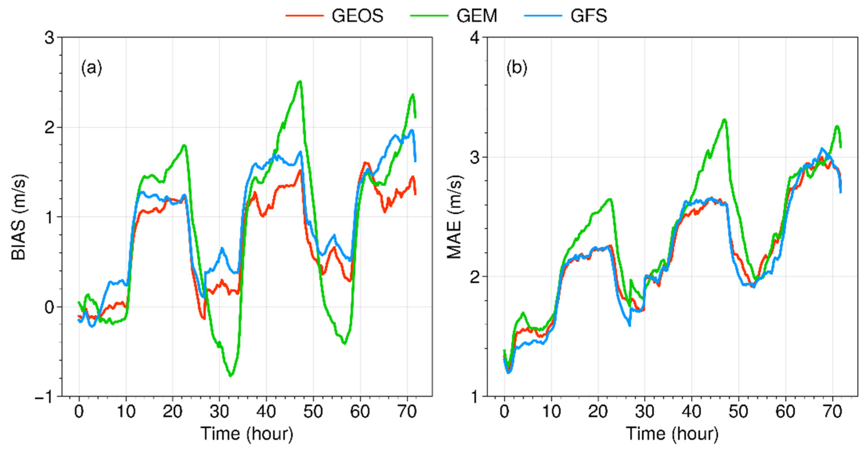
3.6. Growth of Forecast Errors with Lead Time

The 0–72 h forecasts of the ensemble groups driven by the GFS, GEOS, and GEM were examined to analyze the growth of the wind forecast errors with the forecast length (Figure 8). The MAE of the wind speed forecasts of the three ensemble member groups increases with the forecast length at a rate of ~0.4 m/s per day for the 3 days (Figure 8a). The MAEs of the wind speed forecasts of the GFS and GEOS groups are rather close to one another, while the GFS group has a slight advantage. The wind speed errors of the GEM group grow faster at nighttime, resulting in MAE of 0.4 m/s and 0.6 m/s more than the other two groups on the first and second days, respectively.
Comparing Figure 8a,b, we can see that the large MAE of the wind forecasts at night was mainly due to the systematic overestimation of the nighttime wind speeds by the model. It is interesting to note that although the MAE of wind forecasts of the GFS and GEOS groups is relatively close, the bias of the wind speed forecasts of the GEOS group is significantly better than that of the GFS group. Figure 8 shows more clearly that the mean wind forecast error of the GEM group has a large diurnal variation, with a large overestimation of positive wind bias in the nighttime and negative bias in the daytime.

4. Summary and Conclusions

In this paper, statistical verification of a mesoscale ensemble numerical weather prediction system was conducted for hub-height wind prediction at 411 wind turbines representing ~130 wind farms. The ensemble system contains 39 forecast members, and is divided into 3 groups driven by the US GFS and GEOS and the Canadian GEM global weather model forecasts. Each group contains the same set of 13 physical perturbations. The verification period was from 1 March to 15 April 2020. This paper analyzes the error characteristics of the mean wind forecasts of the three ensemble groups and compares their performance. The error statistics (CC, BIAS, and MAE) of the wind forecasts—including the diurnal variability, differences in seven geographical regions, dependence on wind speed regimes, and growth by forecast time—are analyzed. The main conclusions of this study are as follows.
(1)
Among the ensemble groups driven by the GFS, GEOS, and GEM global weather model forecasts, the GFS group significantly outperformed the other two groups with respect to the CC and MAE of the wind forecasts, with 59–64% of the turbines performing best. The GEM group was poorer overall, with only 2% of turbines achieving the best prediction. The wind forecast MAE of the GEOS group was similar to that of the GFS group, but the GEOS group tended to perform better in terms of BIAS. In the GEOS group, there were some larger positive and negative biases that offset one another, resulting in a smaller overall bias;
(2)
All three ensemble groups overestimated the low wind speed (0–3 m/s) and underestimated the high wind speed. All three groups had better forecasts for the wind speeds ranging from 3 to 12 m/s, and the errors of the GFS and GEOS groups were similar. For wind speeds greater than 12 m/s, the GFS group outperformed the GEOS group, and the GEM group had the largest error. The average deviation of the wind forecasts from the observations increased approximately linearly with the magnitude of wind speeds, reaching more than −4 m/s for the cases of strong winds over 15 m/s;
(3)
The wind speed forecasts of all three ensemble groups exhibited similar diurnal variation in each of the seven subregions. The wind forecast bias was generally small during daytime but overestimated by 1–1.5 m/s at night. The GFS group had the best performance, the GEOS group was slightly worse, and the GEM group significantly underestimated the wind speed during daytime. The GEOS group had more accurate wind speed forecasts than the GFS group in nighttime in several complex terrain areas;
(4)
The errors of the wind forecasts of the three ensemble groups increased with forecast lead time, with a growth rate of ~0.3 m/s for the 3-day forecast period. The nighttime MAE was 0.6–0.5 m/s higher than that in the daytime. The MAEs of wind forecasts of the GFS and GEOS groups were relatively close to one another, and the GFS group had a slight advantage. The wind speed forecast errors of the GEM group grew much faster at night, and its biases were ~0.4–0.6 m/s larger than those of the other two groups. The large MAE of the GEM group wind forecast during nighttime was mainly due to the systematic overestimation of wind speed at night;
(5)
Based on the results of this study, the ensemble outputs should first be processed to remove the bias of the three subgroups separately before they are combined for deriving probabilistic wind power forecast products. The model post-processing should be done for each region, as best as possible, for each wind turbine site independently, in order to deal with the unique forecast error properties of the ensembles in different regions. Model developers should devote their attention to mitigating the trend of the wind forecast bias growth with wind speeds.

5. Discussion

It should be noted that the performance of numerical weather models is highly reliant on model resolution [18], regional climate [19], topography [20], underlying land-surface and soil properties [19], weather measurements [21] and data assimilation schemes for model initiation [23], as well as the lateral boundary conditions for limited-area models [24]. The ensemble forecasts overestimate wind speeds. Similar results have also been reported in several previous studies using the WRF model over different global regions [24,36,38]. Although several studies have tried to identify the physical reasons for this, they have not reached a consensus on the issue. From the dynamical point of view, the height and roughness of the subsurface may not be sufficiently considered in the WRF model [69,70], and from the thermodynamic point of view, the WRF model may misestimate the cloudiness, making it difficult to predict the long- and short-wave radiation accurately, and resulting in the misestimation of near-surface wind speed [71,72,73]. Our results show that, driven by different global model forecasts, the BIAS properties of the WRF forecasts differ, but the overall BIAS trends are the same for all subregions in the studied domain.
This study focused on the wind forecast error characteristics of the Inner Mongolia mesoscale ensemble forecasting system with respect to the impact of the ensemble members driven by different global numerical weather prediction model forecasts. Our findings provide a basis for developing a statistical post-processing of the ensemble forecasts to improve wind and power forecasting for the wind farms, and for further improvement of the forecast capability of the WRF models in the future.
However, the present study was based on only 45 days of wind prediction data in the spring of 2020, making it insufficient to describe the year-round forecast error pattern. We are collecting more data to expand this work to a full-year period, and studying the seasonal variation patterns of wind forecast error statistics. Furthermore, this ensemble forecast system contains 10 perturbed members of the varying atmospheric boundary layer parameterization scheme. We are currently analyzing and comparing the error characteristics of the wind forecasts using these different atmospheric boundary layer parameterization schemes; the results will be reported in a separate paper.

Author Contributions

Conceptualization, J.S., Y.L. (Yubao Liu) and X.F.; methodology, Y.L. (Yubao Liu) and Y.L. (Yang Li); software, J.S.; validation, L.S. and X.F.; formal analysis, J.S.; investigation and resources, Y.L. (Yuewei Liu); data curation, J.S., L.S. and G.R.; writing—original draft preparation, J.S.; writing—review and editing, Y.L. (Yubao Liu) and Y.L. (Yang Li); visualization, J.S. and Y.L. (Yang Li); funding acquisition, Y.L. (Yubao Liu) and X.F. All authors have read and agreed to the published version of the manuscript.

Funding

This research was funded by the Jibei Electric Power Company (Grant #520120210003), the Inner Mongolia Electric Power Company, and the Northwest Region Weather Modification Capability Development Program, RQC19081 and RQC-19176.

Institutional Review Board Statement

Not applicable.

Informed Consent Statement

Not applicable.

Data Availability Statement

Not applicable.

Acknowledgments

We give thanks to the Inner Mongolia Meteorological Bureau, the US National Center for Atmospheric Research (NCAR), and Nanjing University of Information Science and Technology (NUIST) for data and computing support.

Conflicts of Interest

The authors declare no conflict of interest.

References

  1. Yu, L.; Zhong, S.; Bian, X.; Heilman, W. Climatology and Trend of Wind Power Resources in China and Its Surrounding Regions: A Revisit Using Climate Forecast System Reanalysis Data. Int. J. Climatol. 2016, 36, 2173–2188. [Google Scholar] [CrossRef]
  2. Makarov, Y.V.; Loutan, C.; Ma, J.; Mello, P.D. Operational impacts of wind generation on California power systems. IEEE Trans. Power Syst. 2009, 24, 1039–1050. [Google Scholar] [CrossRef]
  3. Georgilakis, P.S. Technical challenges associated with the integration of wind power into power systems. Renew. Sustain. Energy Rev. 2008, 12, 852–863. [Google Scholar] [CrossRef] [Green Version]
  4. Smith, J.C.; Milligan, M.R.; DeMeo, E.A.; Parsons, B. Utility wind integration and operating impact state of the art. IEEE Trans. Power Syst. 2007, 22, 900–908. [Google Scholar] [CrossRef]
  5. Shen, X.; Zhou, C.; Fu, X. Study of Time and Meteorological Characteristics of Wind Speed Correlation in Flat Terrains Based on Operation Data. Energies 2018, 11, 219. [Google Scholar] [CrossRef] [Green Version]
  6. Zhang, S.; Liu, Y.; Wang, J.; Wang, C. Research on Combined Model Based on Multi-Objective Optimization and Application in Wind Speed Forecast. Appl. Sci. 2019, 9, 423. [Google Scholar] [CrossRef] [Green Version]
  7. Geng, D.; Zhang, H.; Wu, H. Short-Term Wind Speed Prediction Based on Principal Component Analysis and LSTM. Appl. Sci. 2020, 10, 4416. [Google Scholar] [CrossRef]
  8. Emeksiz, C.; Tan, M. Multi-step wind speed forecasting and Hurst analysis using novel hybrid secondary decomposition approach. Energy 2022, 238, 121764. [Google Scholar] [CrossRef]
  9. Jiang, P.; Liu, Z.; Niu, X.; Zhang, L. A combined forecasting system based on statistical method, artificial neural networks, and deep learning methods for short-term wind speed forecasting. Energy 2021, 217, 119361. [Google Scholar] [CrossRef]
  10. Neshat, M.; Nezhad, M.M.; Abbasnejad, E.; Mirjalili, S.; Tjernberg, L.B.; Garcia, D.A.; Alexander, B.; Wagner, M. A deep learning-based evolutionary model for short-term wind speed forecasting: A case study of the Lillgrund offshore wind farm. Energy Convers. Manag. 2021, 236, 114002. [Google Scholar] [CrossRef]
  11. Li, D.; Jiang, F.; Chen, M.; Qian, T. Multi-step-ahead wind speed forecasting based on a hybrid decomposition method and temporal convolutional networks. Energy 2022, 238, 121981. [Google Scholar] [CrossRef]
  12. Bauer, P.; Thorpe, A.; Brunet, G. The Quiet Revolution of Numerical Weather Prediction. Nature 2015, 525, 47–55. [Google Scholar] [CrossRef] [PubMed]
  13. Alharbi, F.R.; Csala, D. Wind Speed and Solar Irradiance Prediction Using a Bidirectional Long Short-Term Memory Model Based on Neural Networks. Energies 2021, 14, 6501. [Google Scholar] [CrossRef]
  14. Chen, Q.; Chen, Y.; Bai, X. Deterministic and Interval Wind Speed Prediction Method in Offshore Wind Farm Considering the Randomness of Wind. Energies 2020, 13, 5595. [Google Scholar] [CrossRef]
  15. Bai, Y.; Tang, L.; Fan, M.; Ma, X.; Yang, Y. Fuzzy First-Order Transition-Rules-Trained Hybrid Forecasting System for Short-Term Wind Speed Forecasts. Energies 2020, 13, 3332. [Google Scholar] [CrossRef]
  16. Zhao, X.; Wei, H.; Li, C.; Zhang, K. A Hybrid Nonlinear Forecasting Strategy for Short-Term Wind Speed. Energies 2020, 13, 1596. [Google Scholar] [CrossRef] [Green Version]
  17. Brahimi, T. Using Artificial Intelligence to Predict Wind Speed for Energy Application in Saudi Arabia. Energies 2019, 12, 4669. [Google Scholar] [CrossRef] [Green Version]
  18. Ren, Y.; Li, H.; Lin, H.-C. Optimization of Feedforward Neural Networks Using an Improved Flower Pollination Algorithm for Short-Term Wind Speed Prediction. Energies 2019, 12, 4126. [Google Scholar] [CrossRef] [Green Version]
  19. Luo, N.; Guo, Y. Impact of Model Resolution on the Simulation of Precipitation Extremes over China. Sustainability 2022, 14, 25. [Google Scholar] [CrossRef]
  20. Zhang, M.; Tölle, M.H.; Hartmann, E.; Xoplaki, E.; Luterbacher, J. A Sensitivity Assessment of COSMO-CLM to Different Land Cover Schemes in Convection-Permitting Climate Simulations over Europe. Atmosphere 2021, 12, 1595. [Google Scholar] [CrossRef]
  21. Zhang, C.; He, J.; Lai, X.; Liu, Y.; Che, H.; Gong, S. The Impact of the Variation in Weather and Season on WRF Dynamical Downscaling in the Pearl River Delta Region. Atmosphere 2021, 12, 409. [Google Scholar] [CrossRef]
  22. Suh, M.S.; Oh, S.G. Impacts of Boundary Conditions on the Simulation of Atmospheric Fields Using RegCM4 over CORDEX East Asia. Atmosphere 2015, 6, 783–804. [Google Scholar] [CrossRef] [Green Version]
  23. Liu, Y.; Warner, T.T.; Bowers, J.F.; Carson, L.P.; Chen, F.; Clough, C.A.; Davis, C.A.; Egeland, C.H.; Halvorson, S.F.; Huck, T.W., Jr.; et al. The Operational Mesogamma-Scale Analysis and Forecast System of the US Army Test and Evaluation Command. Part I: Overview of the Modeling System, the Forecast Products, and How the Products are Used. J. Appl. Meteorol. Climatol. 2008, 47, 1077–1092. [Google Scholar] [CrossRef] [Green Version]
  24. Draxl, C.; Hahmann, A.N.; Peña, A.; Giebel, G. Evaluating Winds and Vertical Wind Shear from Weather Research and Forecasting Model Forecasts Using Seven Planetary Boundary Layer Schemes. Wind Energy 2014, 17, 39–55. [Google Scholar] [CrossRef]
  25. Li, S.; Wang, Y.; Yuan, H.; Song, J.; Xu, X. Ensemble mean forecast skill and applications with the T213 ensemble prediction system. Adv. Atmos. Sci. 2016, 33, 1297–1305. [Google Scholar] [CrossRef]
  26. Dube, A.; Ashrit, R.; Singh, H.; Arora, K.; Iyengar, G.; Rajagopal, E.N. Evaluating the performance of two global ensemble forecasting systems in predicting rainfall over India during the southwest monsoons. Meteorol. Appl. 2017, 24, 230–238. [Google Scholar] [CrossRef] [Green Version]
  27. Rabier, F.; Klinker, E.; Courtier, P.; Hollingsworth, A. Sensitivity of Forecast Error to Initial Conditions. Q. J. R. Meteorol. Soc. 1996, 122, 121–150. [Google Scholar] [CrossRef]
  28. Buizza, R.; Miller, M.; Palmer, T.N. Stochastic Representation of Model Uncertainties in the ECMWF Ensemble Prediction System. Q. J. R. Meteorol. Soc. 1999, 125, 2887–2908. [Google Scholar] [CrossRef]
  29. Lorenz, E.N. Deterministic Nonperiodic Flow. J. Atmos. Sci. 1963, 20, 130–141. [Google Scholar] [CrossRef] [Green Version]
  30. Leith, C.E. Theoretical skill of Monte Carlo Forecasts. Mon. Weather Rev. 1974, 102, 409–418. [Google Scholar] [CrossRef] [Green Version]
  31. Du, J.; Mullen, S.L.; Sanders, F. Short-Range Ensemble Forecasting of Quantitative Precipitation. Mon. Weather Rev. 1997, 125, 2427–2459. [Google Scholar] [CrossRef]
  32. Baldauf, M.; Seifert, A.; Foerstner, J.; Majewski, D.; Raschendorfer, M.; Reinhardt, T. Operational Convective-Scale Numerical Weather Prediction with the Cosmo Model: Description and Sensitivities. Mon. Weather Rev. 2011, 139, 3887–3905. [Google Scholar] [CrossRef]
  33. Eckel, F.A.; Mass, C.F. Aspects of Effective Mesoscale, Short-Range Ensemble Forecasting. Weather Forecast 2005, 20, 328–350. [Google Scholar] [CrossRef]
  34. Han, J.; Pan, H. Revision of Convection and Vertical Diffusion Schemes in the NCEP Global Forecast System. Weather Forecast 2011, 26, 520–533. [Google Scholar] [CrossRef]
  35. Pinson, P.; Hagedorn, R. Verification of the ECMWF Ensemble Forecasts of Wind Speed against Analyses and Observations. Meteorol. Appl. 2012, 19, 484–500. [Google Scholar] [CrossRef] [Green Version]
  36. Xie, B.; Fung, J.C.H.; Chan, A.; Lau, A. Evaluation of Nonlocal and Local Planetary Boundary Layer Schemes in the WRF Model. J. Geophys. Res. Atmos. 2012, 117, 1–26. [Google Scholar] [CrossRef]
  37. Mass, C.F.; Warner, M.D.; Steed, R. Strong Westerly Wind Events in the Strait of Juan de Fuca. Weather Forecast 2014, 29, 445–465. [Google Scholar] [CrossRef]
  38. Zhang, D.; Zheng, W. Diurnal Cycles of Surface Winds and Temperatures as Simulated by Five Boundary Layer Parameterizations. J. Appl. Meteorol. Climatol. 2004, 43, 157–169. [Google Scholar] [CrossRef] [Green Version]
  39. Ancell, B.C.; Mass, C.F.; Hakim, G.J. Evaluation of Surface Analyses and Forecasts with a Multiscale Ensemble Kalman Filter in Regions of Complex Terrain. Mon. Weather Rev. 2011, 139, 2008–2024. [Google Scholar] [CrossRef]
  40. Carvalho, D.; Rocha, A.; Gómez-Gesteira, M.; Santos, C. A Sensitivity Study of the WRF Model in Wind Simulation for an Area of High Wind Energy. Environ. Model. Softw. 2012, 33, 23–34. [Google Scholar] [CrossRef] [Green Version]
  41. Coniglio, M.C.; Correia, J., Jr.; Marsh, P.T.; Kong, F. Verification of Convection-Allowing WRF Model Forecasts of the Planetary Boundary Layer Using Sounding Observations. Weather Forecast 2013, 28, 842–862. [Google Scholar] [CrossRef]
  42. Serafin, S.; Adler, B.; Cuxart, J.; De Wekker, S.F.J.; Gohm, A.; Grisogono, B.; Kalthoff, N.; Kirshbaum, D.J.; Rotach, M.W.; Schmidli, J.; et al. Exchange Processes in the Atmospheric Boundary Layer over Mountainous Terrain. Atmosphere 2018, 9, 102. [Google Scholar] [CrossRef] [Green Version]
  43. Rife, D.L.; Davis, C.A. Verification of Temporal Variations in Mesoscale Numerical Wind Forecasts. Mon. Weather Rev. 2005, 133, 3368–3381. [Google Scholar] [CrossRef]
  44. Brewer, M.C.; Mass, C.F. Simulation of Summer Diurnal Circulations over the Northwest United States. Weather Forecast 2014, 29, 1208–1228. [Google Scholar] [CrossRef]
  45. Brewer, M.C.; Mass, C.F. Projected Changes in Western U.S. Large-Scale Summer Synoptic Circulations and Variability in CMIP5 Models. J. Clim. 2016, 29, 5965–5978. [Google Scholar] [CrossRef]
  46. Warner, M.D.; Mass, C.F. Changes in the Climatology, Structure, and Seasonality of Northeast Pacific Atmospheric Rivers in CMIP5 Climate Simulations. J. Hydrometeorol. 2017, 18, 2121–2141. [Google Scholar] [CrossRef]
  47. Weber, N.J.; Mass, C.F. Evaluating the Subseasonal to Seasonal CFSv2 Forecast Skill with an Emphasis on Tropical Convection. Mon. Weather Rev. 2017, 146, 3795–3815. [Google Scholar] [CrossRef]
  48. Xu, W.; Ning, L.; Luo, Y. Wind Speed Forecast Based on Post-Processing of Numerical Weather Predictions Using a Gradient Boosting Decision Tree Algorithm. Atmosphere 2020, 11, 738. [Google Scholar] [CrossRef]
  49. Fernández-González, S.; Sastre, M.; Valero, F.; Merino, A.; García-Ortega, E.; Sánchez, J.L.; Lorenzana, J.; Martín, M.L. Characterization of Spread in a Mesoscale Ensemble Prediction System: Multiphysics versus Initial Conditions. Meteorol. Z. 2018, 28, 59–67. [Google Scholar] [CrossRef]
  50. Mass, C.F.; David, O. The Northern California Wildfires of October 8–9, 2017: The Role of a Major Downslope Windstorm Event. Bull. Am. Meteorol. Soc. 2019, 100, 235–256. [Google Scholar] [CrossRef]
  51. Zhang, T.; Zhao, C.; Gong, C.; Pu, Z. Simulation of Wind Speed Based on Different Driving Datasets and Parameterization Schemes Near Dunhuang Wind Farms in Northwest of China. Atmosphere 2020, 11, 647. [Google Scholar] [CrossRef]
  52. Gao, Y.; Ma, S.; Wang, T.; Wang, T.; Gong, Y.; Peng, F.; Tsunekawa, A. Assessing the wind energy potential of China in considering its variability/intermittency. Energy Convers. Manag. 2020, 226, 113580. [Google Scholar] [CrossRef]
  53. Knievel, J.C.; Liu, Y.; Hopson, T.M.; Shaw, J.S.; Halvorson, S.F.; Fisher, H.H.; Roux, G.; Sheu, R.-S.; Pan, L.; Wu, W.; et al. Mesoscale Ensemble Weather Prediction at U.S. Army Dugway Proving Ground, Utah. Weather Forecast 2017, 32, 2195–2216. [Google Scholar] [CrossRef]
  54. Kosovic, B.; Haupt, S.E.; Adriaansen, D.; Alessandrini, S.; Wiener, G.; Delle Monache, L.; Liu, Y.; Linden, S.; Jensen, T.; Cheng, W.; et al. A Comprehensive Wind Power Forecasting System Integrating Artificial Intelligence and Numerical Weather Prediction. Engergies 2020, 13, 1372. [Google Scholar] [CrossRef] [Green Version]
  55. Pan, L.; Liu, Y.; Roux, G.; Cheng, W.; Liu, Y.; Hu, J.; Jin, S.; Feng, S.; Du, J.; Peng, L. Seasonal Variation of the Surface Wind Forcast Performance of the High-Resolution WRF-RTFDDA System over China. Atmos. Res. 2021, 259, 105673. [Google Scholar] [CrossRef]
  56. Mahoney, W.P.; Parks, K.; Wiener, G.; Liu, Y.; Myers, W.; Sun, J.; Monache, L.-D.; Hopson, T.; Johnson, D.; Haupt, S.E. A Wind Power Forecasting System to Optimize Grid Integration. IEEE Trans. Sustain. Energy 2012, 3, 670–682. [Google Scholar] [CrossRef]
  57. Cheng, W.Y.Y.; Liu, Y.; Liu, Y.W.; Zhang, Y.; Mahoney, W.P.; Warner, T.T. The Impact of Model Physics on Numerical Wind Forecasts. Renew. Energy 2013, 55, 347–356. [Google Scholar] [CrossRef]
  58. Cheng, W.Y.Y.; Liu, Y.; Bourgeois, A.; Wu, Y.; Haupt, S.E. Short-Term Wind Forecast of a Data Assimilation/Weather Forecasting System with Wind Turbine Anemometer Measurement Assimilation. Renew. Energy 2017, 107, 340–351. [Google Scholar] [CrossRef]
  59. Hong, S.-Y.; Noh, Y.; Dudhia, J. A New Vertical Diffusion Package with an Explicit Treatment of Entrainment Processes. Mon. Weather Rev. 2006, 134, 2318–2341. [Google Scholar] [CrossRef] [Green Version]
  60. Bougeault, P.; Lacarrere, P. Parameterization of Orography-Induced Turbulence in a Mesobeta—Scale Model. Mon. Weather Rev. 1989, 117, 1872–1890. [Google Scholar] [CrossRef]
  61. Nakanishi, M.; Niino, H. An Improved Mellor-Yamada Level 3 Model: Its Numerical Stability and Application to a Regional. Bound. Layer Meteorol. 2006, 119, 397–407. [Google Scholar] [CrossRef]
  62. Janjić, Z.I. The Step-Mountain Eta Coordinate Model: Further Developments of the Convection, Viscous Sublayer, and Turbulence. Mon. Weather Rev. 1994, 122, 927–945. [Google Scholar] [CrossRef] [Green Version]
  63. Shin, H.H.; Hong, S.Y. Representation of the Subgrid-Scale Turbulent Transport in Convective Boundary Layers at Gray-Zone Resolutions. Mon. Weather Rev. 2015, 143, 250–271. [Google Scholar] [CrossRef]
  64. Angevine, W.M.; Jiang, H.; Mauritsen, T. Performance of an Eddy Diffusivity-Mass Flux Scheme for Shallow Cumulus Boundary Layers. Mon. Weather Rev. 2010, 138, 2895–2912. [Google Scholar] [CrossRef] [Green Version]
  65. Bretherton, C.S.; Park, S. A New Moist Turbulence Parameterization in the Community Atmosphere Model. J. Clim. 2009, 22, 3422–3448. [Google Scholar] [CrossRef]
  66. Grenier, H.; Bretherton, C.S. A Moist PBL Parameterization for Large-Scale Models and Its Application to Subtropical Cloud. Mon. Weather Rev. 2001, 129, 357–377. [Google Scholar] [CrossRef] [Green Version]
  67. Sukoriansky, S.; Perov, V.; Galperin, B. Application of a New Spectral Model of Stratified Turbulence to the Atmospheric Boundary Layer over Sea Ice. Bound. Layer Meteorol. 2005, 117, 231–257. [Google Scholar] [CrossRef]
  68. Sedaghat, A.; Hassanzadeh, A.; Jamali, J.; Mostafaeipour, A.; Chen, W. Determination of rated wind speed for maximum annual energy production of variable speed wind turbines. Appl. Energy 2017, 205, 781–789. [Google Scholar] [CrossRef]
  69. Hahmann, A.N.; Lennard, C.; Badger, J.; Vincent, C.L.; Kelly, M.C.; Volker, P.J.; Argent, B.; Refslund, J. Mesoscale modeling for the Wind Atlas of South Africa (WASA) project. DTU Wind Energy 2014, 50, 80. [Google Scholar]
  70. Floors, R.; Vincent, C.L.; Gryning, S.E.; Peña, A.; Batchvarova, E. The wind profile in the coastal boundary layer: Wind lidar measurements and numerical modelling. Bound.-Layer Meteorol. 2013, 147, 469–491. [Google Scholar] [CrossRef]
  71. Ruiz-Arias, J.A.; Arbizu-Barrena, C.; Santos-Alamillos, F.J.; Tovar-Pescador, J.; Pozo-Vázquez, D. Assessing the surface solar radiation budget in the WRF model: A spatiotemporal analysis of the bias and its causes. Mon. Weather Rev. 2016, 144, 703–711. [Google Scholar] [CrossRef]
  72. Mahrt, L. The early evening boundary layer transition. Q. J. R. Meteorol. Soc. 1981, 107, 329–343. [Google Scholar] [CrossRef]
  73. Varquez, A.C.G.; Nakayoshi, M.; Makabe, T.; Kanda, M. WRF Application of High Resolution Urban Surface Parameters on Some Major Cities of Japan. J. Jpn. Soc. Civil Eng. Ser. B1 Hydraul. Eng. 2014, 170, I_175–I_180. [Google Scholar] [CrossRef] [Green Version]
Figure 1. (a) Schematic diagram of the ensemble prediction domains for wind farms in the Inner Mongolia Autonomous Region. The horizontal resolution of the coarse-grid simulation domain is 13.5 km, and the horizontal resolution of the two-nested fine-grid simulation domain is 2.7 km. The colored background is the terrain. (b) Topography (color filled map) and distribution of test stations (black dots) in the study area. The black line in (b) marks the provincial boundary of the Inner Mongolia Autonomous Region, while Areas 1–7 mark the seven subregions enclosed by cyan-colored rectangles.
Energies 15 00896 g001
Figure 2. Diurnal variation in the observed wind speeds for the seven sub-areas. The red line is the median value, dark blue is 25–75%, and the light blue zone (including dark blue zone) is 5–95%. The x-axis represents the time (UTC).
Energies 15 00896 g002
Figure 3. Distribution of the sites colored for the dominant best performing ensemble groups driven by the GFS, GEOS, and GEM forecasts: (a) correlation coefficients, (b) mean absolute errors, and (c) biases.
Energies 15 00896 g003
Figure 4. (a) BIAS and (b) MAE of the wind forecasts of the ensemble groups driven by the GFS, GEOS, and GEM. The line charts are the error statistics, and the histograms correspond to the number of data samples.
Energies 15 00896 g004
Figure 5. (a) Diurnal variation in wind speed observations and forecasts, and (b) MAE of the ensemble groups driven by the GFS, GEOS, and GEM. The x-axis represents the time (UTC).
Energies 15 00896 g005
Figure 6. Boxplots of the wind forecast bias distributions for the ensemble groups driven by the GFS, GEOS, and GEM forecasts for daytime (00:00–10:00 UTC), sunset (10:00–12:00 UTC), nighttime (12:00–22:00 UTC), and sunrise (22:00–00:00 UTC). The black horizontal line marks the median bias, while the white triangle represents the mean bias.
Energies 15 00896 g006
Figure 7. The BIAS of the wind forecasts of the three ensemble groups in the seven sub-areas. The x-axis represents the time (UTC).
Energies 15 00896 g007
Figure 8. Variation in wind speed forecast errors with forecast time for the ensemble groups driven by the three global model forecasts: (a) BIAS and (b) MAE. The x-axis represents the time (hours).
Energies 15 00896 g008
Table 1. Mesoscale ensemble prediction member names and parameterization scheme configuration.
Member NameMember Perturbations
CTRLYSU PBL [59]
BOUBouLac PBL [60]
MYNN2MYNN 2.5 level TKE scheme [61]
MYJMellor–Yamada–Janjic TKE PBL scheme [62]
SHSShin–Hong ‘scale-aware’ PBL scheme [63]
TEMFTEMF (Total Energy Mass Flux) scheme [64]
UNWUW boundary layer scheme from CAM5 [65]
GBMGrenier–Bretherton–McCaa scheme [66]
QNSEddy-diffusivity mass flux, quasi-normal scale elimination PBL [67]
SKEBAStochastic kinetic energy backscatter scheme A
SKEBBStochastic kinetic energy backscatter scheme B
SKEBCStochastic kinetic energy backscatter scheme C
RRMGMorrison Microphysics + Mellor–Yamada–Janjic PBL scheme
Table 2. Statistical verification of all stations for the GFS, GEOS, and GEM groups (45 days).
GEOS GroupGEM GroupGFS Group
MeanMaxMedianMinMeanMaxMedianMinMeanMaxMedianMin
CC0.680.660.620.580.640.630.580.530.700.670.650.61
BIAS (m/s)+0.56+0.75+0.60−0.05+0.76+0.91+0.79+0.15+0.67+0.91+0.69+0.04
MAE (m/s)1.842.132.061.861.992.322.151.991.812.102.031.80
Table 3. Ranking statistics of wind speed forecast errors for the three ensemble forecast groups driven by the GFS, GEOS, and GEM model forecasts.
GEOS GroupGEM GroupGFS Group
NBPS */R *NWPS */RNBPS/RNWPS/RNBPS/RNWPS/R
CC141/34.3%81/19.7%8/1.9%318/77.4%262/63.7%12/2.9%
BIAS315/76.6%28/6.8%27/6.6%315/76.6%69/16.8%68/16.5%
MAE152/37.0%47/11.4%9/2.2%355/86.4%241/58.6%9/2.2%
* NBPS: # of best performing stations; NWPS: # of worst performing stations; R: ratio with reference to the total.
Publisher’s Note: MDPI stays neutral with regard to jurisdictional claims in published maps and institutional affiliations.

