A Self-Validating Method via the Unification of Multiple Models for Consistent Parameter Identification in PEM Fuel Cells

Abstract

Mathematical models are used for simulating the electrochemical phenomena of proton-exchange-membrane (PEM) fuel cells. They differ in the scale, modeling variables, precision in specific features, and the required parameters. Often, the input parameters are not measurable and need to be estimated by minimizing the error between the model output and experimental data; however, the estimated parameters could differ from one model to another, hence provoking uncertainty about the correct values and the model’s suitability for simulating the real phenomenon. To address these issues, we introduced a self-validating methodology using three different mathematical models: The first set of parameters was estimated with a semi-empirical (SE) model; then, it was used for computing several points of the polarization curve (PC). The SE parameters and points were used to estimate a second set of parameters and to compute a single point of the PC with a macro-homogeneous (MH) model. The parameters and concentration profiles from the MH solution were used to estimate the last set of parameters with the reaction–convection–diffusion (SP-RCD) model, increasing the detail of the simulation. The SP-RCD parameters were returned to the MH model to recover the complete PC. The proposed methodology requires a few data points to consistently recover the same PC from the three models through estimating parameters in one model and validating them in the others. As output, the method provides complete information about several variables and the physical properties of the catalysts. In addition to the consistent simulation, the numerical results are consistent with those reported in the literature, thus validating the proposed method.

1. Introduction

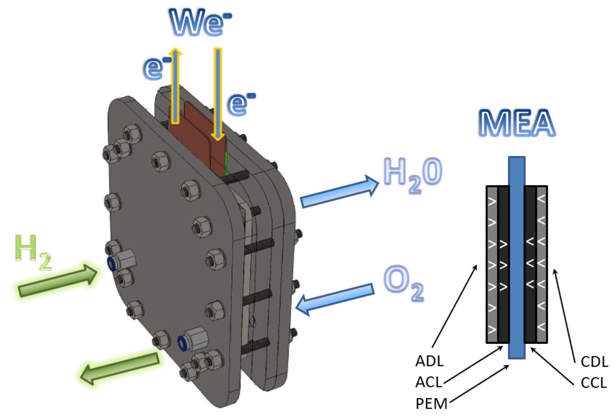
Since the 20th century and the beginning of the 21st century, the generation of alternative clean technologies has been increasing to counteract the increase in pollutants and energy consumption due to the increasing global population [1]. The PEM fuel cells are clean devices that directly generate electrical energy, water, and heat through electrochemical reactions in their cathodic and anodic compartments, as shown in Figure 1. The electrochemical reactions in a PEMFC are represented in Equations (1) to (3) [2,3]:

Anode reaction:

$$H_2\to 2H^{+}+2e^{-},(E_{an}^0=0Vvs.SHE).$$

(1)

Cathode reaction:

$$\frac{1}{2}{O}_2+2H^{+}+2e^{-}\to H_{2}O,(E_{cat}^0=1.23Vvs.SHE).$$

(2)

Global reaction:

$$H_2+\frac{1}{2}{O}_2\to H_{2}O,(E_{cell}^0=1.23Vvs.SHE).$$

(3)

The mathematical modeling of fuel cells allows us to study the energy conversion processes inside of a PEM fuel cell; analyze designs, structures, or material composition; and improve electrical energy generation. Several mathematical models have been implemented and validated through laboratory experimentation in the literature. Among the models, the following stand out: (a) Empirical and semi-empirical models: These models are based on algebraic expressions obtained from physical relations present in the PEMFC. They model the behavior of the polarization curves using a set of empirical or semi-empirical parameters through non-linear regression methods [2,4,5]. (b) Interface models: These models’ diffusion processes occur through the anode, membrane, and cathode using diffusion differential equations, assuming that the catalytic layer is negligible [6,7,8]. (c) Macro-homogeneous models: These consist of a set of non-linear ordinary differential equations based on the assumption that the main reactions occur in the catalytic layer of the cathode and analyze the physical compositions of the materials and their properties [9,10,11,12,13,14]. (d) Agglomerated models: These consist of partial differential equations, model diffusion processes, and involve a description of the physical composition of the cathodic catalytic layer, its porosity, or catalyst conglomerates [15,16,17].

In the modeling and simulation of PEMFC, mathematical models require a set of parameters that are not obtained experimentally, such as diffusion coefficients; hence, they need to be estimated [2,12,13,15]. The parameter estimation problem is an optimization problem with an objective function defined by the error minimization of the fitting experimental data and the model output [5,18,19,20]. Algorithms for solving the parameter estimation problem in PEMFC are particle swarm optimization (PSO) [21,22], the artificial immune system [23], simulated annealing [2,18], the genetic algorithm (GA) [5,24], the RNA-genetic algorithm [19], the differential evolution algorithm [25,26], the artificial bee swarm [27], fuzzy logic control [28], harmonic search in [29], JAYA-NM [30], the Grasshopper Optimization Algorithm (GOA) [31], the Salp Swarm Optimizer (SSO) [32], moth–flame optimization [33], and UMDA${}^G$ [34], among others. In general, most of them report acceptable solutions; nevertheless, they vary in the consistency of their results, that is, in delivering similar estimated parameters for the same conditions in several independent executions. UMDA${}^G$ [34] has shown a reliable balance between the precision of the approximation and the computational cost and consistency. Consequently, it was used in this work for the estimation task.

In this context, the contributions of this article are various. First, we unified three high-performing models to demonstrate how to simulate the same cell with all of them; from our point of view, the main advantage of these multiple simulations is that the models corroborate that the parameters are the correct ones and deliver information about the cell performance, which is not possible to measure but is obtained from the simulation. Second, we estimated parameters in one model using a few experimental data, and then we used the other models to increase the precision of the estimation and to corroborate that the parameters reproduce the cell performance. Third, we reproduced incomplete experimental information. Once the parameters had been estimated, we were able to reproduce the full polarization curves and concentration profiles. Fourth, we presented the assembly of numerical techniques as a complete method for parameter estimation and multimodel simulation of the PEMFC.

The paper is organized as follows: Section 2 presents an overview of the three selected mathematical models; we describe their advantages and disadvantages. In Section 3, we present the parameter estimation problem. Our proposed self-validating methodology is presented in Section 4. In Section 5, we show the numerical and comparative results of our proposal with those reported in the literature. Finally, a conclusion of this work is presented in Section 6.

2. Mathematical Models for PEMFC

In this section, we describe the three mathematical models used: semi-empirical, macro-homogeneous, and SP-RCD models; each of them requires a different set of parameters but shares some of them, and each delivers different kinds of solutions that, according to the methodology introduced in this work, are interrelated for the consistent simulation of the PEMFC and the consistent estimation of parameters.

Table 1. List of important variables of the mathematical models.

Symbol	General Parameters	Symbol	MH and SP-RCD Parameters
$E_{Nernst}$	open circuit voltage (V)	$C_{0,ref}$	Reference oxygen concentration (mol cm${}^{-3}$)
${\eta }_{act}$	activation voltage drop (V)	${\alpha }_c$	Cathodic electron transfer coefficient
${\eta }_{Ohmic}$	Ohmic voltage drop (V)	${\alpha }_a$	Anodic electron transfer coefficient
${\eta }_{con}$	concentration voltage drop (V)	$C_H$	Hydrogen concentration (mol cm${}^{-3}$)
$V_{FC}$	stack voltage (V)	$A_s$	Surface area per unit mass of Pt (cm${}^2$ g${}^{-1}$)
n	number of cells connected in series	$i_{0,ref}$	Reference exchange current density (A cm${}^{-2}$)
	Operational parameters	${ϵ}_c$	Void volume fraction, or CL porosity
T	temperature (K)	${\gamma }_{O_2}$	Order of the oxygen reduction reaction
$P_{H_2}$	partial pressure of hydrogen (atm)	${\kappa }^{eff}$	Effective protonic conductivity (S cm${}^{-1}$)
$P_{O_2}$	partial pressure of oxygen (atm)	$\kappa$	Bulk protonic conductivity (S cm${}^{-1}$)
$R{H}_c$	relative humidity of vapor in the cathode	${\sigma }^{eff}$	Effective solid electronic conductivity (S cm${}^{-1}$)
$R{H}_a$	relative humidity of vapor in the anode	$\sigma$	Solid electronic conductivity (S cm${}^{-1}$)
$P_a$	inlet pressures at the anode (atm)	$L_c$	Thickness of the CL ($\mathsf{\mu }m$)
$P_c$	inlet pressures at the cathode (atm)	$L_{m,c}$	Volume fraction of the ionomer phase
$C_{O_2}$	oxygen concentration (mol cm${}^{-3}$)	$L_s$	Volume fraction of solid portion of the GDL
	Semi-empirical parameters	${ϵ}_g$	GDL porosity
B	parametric coefficient	$D_{O_2-w}^{eff}$	Oxygen effective diffusion coefficient in
${\rho }_M$	specific membrane resistivity ($\Omega$ cm)		The water-flooded void region (cm${}^2$ s${}^{-1}$)
i	cell current (A)	$D_{O_2-m}$	Oxygen diffusion coefficient (cm${}^2$ s${}^{-1}$)
$I_{\delta }$	current density (A cm${}^{-2}$)	${\rho }_C$	Carbon density (g cm${}^{-3}$)
$I_{max}$	maximum current density (A cm${}^{-2}$)	$m_{Pt}$	Mass loading of Pt per unit area (mg cm${}^2$)
A	active cell area (cm${}^2$)	$m_C$	Mass loading of C per unit area (mg cm${}^{-2}$)
$R_M$	equivalent membrane resistance ($\Omega$)	f	Platinum mass fraction in the Pt/C catalyst
$\psi$	parameter related to the water in the PEM	${\rho }_{Pt}$	Platinum density (g cm${}^{-3}$)
$L_c$	membrane thickness (cm)
$R_C$	equivalent contact resistance ($\Omega$)
${\xi }_i$	semi-empirical coefficient ($i=1,..,4$)

shows the nomenclature of the principal parameters for the three models.

2.1. Semi-Empirical Model

The semi-empirical model is described by algebraic expressions as functions of operational parameters that, through the estimation of so-called semi-empirical parameters, allow the fitting of a simulated polarization curve to experimental data [30,32,34]. The model uses operational parameters, such as the pressures of gases in the cell, the active area of the catalyst, or the thickness.

Table 2. Semi-empirical mathematical model; details in [4].

Cell voltage (V)	$$\begin{gathered} V_{FC}=E_{Nernst}-{\eta }_{act}-{\eta }_{Ohmic}-{\eta }_{con} \\ {E}_{Nernst}=1.229-0.85\times {10}^{-3}(\mathrm{T}-298.15) \\ +4.31\times {10}^{-5}\mathrm{T}\left[\ln \left({\mathrm{P}}_{{\mathrm{H}}_2}\right)+1/2ln\left({\mathrm{P}}_{{\mathrm{O}}_2}\right)\right] \end{gathered}$$
Activation overpotential	$$\begin{gathered} {\eta }_{act}=-[{\xi }_1+{\xi }_{2}T+{\xi }_{3}Tln\left(C_{O_2}\right)+{\xi }_{4}Tln\left(i\right)] \\ {C}_{O_2}=\frac{P_{O_2}}{5.08\times {10}^6\times e^{-(498/T)}},C_{H_2}=\frac{P_{H_2}}{1.09\times {10}^6\times e^{-(77/T)}}, \\ {\xi }_2=2.86e^{-3}+2e^{-4}ln\left(A\right)+\left(4.3e^{-5}\right)ln\left(C_{H_2}\right) \end{gathered}$$
Ohmic overpotential	$$\begin{gathered} {\eta }_{Ohmic}=i(R_M+R_C), \\ {R}_M=\frac{{\rho }_M\times L_c}{A}, \\ {\rho }_M=\frac{181.6[1+0.03·(i/A)+0.062·{(T/303)}^2·{(i/A)}^2]}{[\psi -0.634-3·(i/A\left)\right]·exp[4.18·(T-303/T\left)\right]}, \end{gathered}$$
Concentration overpotential	${\eta }_{con}=-B·\left(1-\frac{I_{\delta }}{I_{max}}\right),$

shows the algebraic expressions that can be used to obtain the PEMFC voltage in terms of the Nernst equation and the activation, ohmic and concentration overpotential losses, as shown in Figure 2. Numerical simulations are used to analyze the behavior under different operational conditions, for instance, if the membrane or pressures are changed.

The results of this model show the general characteristics of the PEMFC but may not be able to provide information about microscopic characteristics, such as density and platinum content in the catalytic layers [36,37]. The most commonly estimated set of parameters is $\overrightarrow{\theta }=\{{\xi }_1,{\xi }_2,{\xi }_3,{\xi }_4,R_c,B,\psi \}$ [23,25,30,34].

The advantages of this model are its adaptability to fit different experimental data with adequate parameter estimation, and it is computationally inexpensive. The main disadvantages are: (1) the result varies in its precision with the number of selected parameters to estimate (physical or semi-empirical parameters); (2) the obtained information only concerns the polarization curve and operational parameters, for instance, reactant gas pressures or active area of the catalysts. The common techniques used in the literature to estimate parameters in this type of model are PSO, GA, and JAYA, among others [22,24,30]. This model is suitable to approximate the complete polarization curve, as shown in Figure 2. These results can be used to feed another model that complements the information for a PEMFC.

2.2. Macro-Homogeneous Model

The macro-homogeneous model is defined by a system of non-linear ordinary differential equations that describes the oxygen concentration, overpotential, and current density through the catalyst layer in the cathode (CL), where the most important reaction of a PEM cell occurs, as shown in Figure 3. The model describes the catalyst layer as a one-dimensional problem in steady-state; its principal advantage is including the characteristics or physical properties of the materials in the catalyst layer, such as platinum density, carbon density, and porosities. The peculiarity of this model is its applicability at low or intermediate current densities. It produces unstable numerical results at high current densities, associated with losses due to concentration, generating spurious solutions [10,12,13].

The standard mathematical model is described by the following nonlinear boundary value problem [10,12,13,14]:

$$\frac{d{O}_2}{dz}=\frac{i-I_{\delta }}{4F{D}_{O_2}^{eff}}$$

(4)

$$\frac{d{\eta }_{act}}{dz}=\frac{i}{{\kappa }^{eff}}+\frac{i-I_{\delta }}{{\sigma }^{eff}}.$$

(5)

$$\frac{di}{dz}=a{i}_0\left[exp\left(\frac{{\alpha }_{c}F}{RT}{\eta }_{act}\right)-exp\left(\frac{{\alpha }_{a}F}{RT}{\eta }_{act}\right)\right],$$

(6)

on $\Omega =[0,l_c]$, where $l_c$ is the thickness of the CL, subject to the boundary conditions:

$$\begin{array}{cc}\hfill z=0,& O_2\left(0\right)=O_2^{*},i\left(0\right)=0\hfill \\ \hfill z=l_c,& i\left(l_c\right)=I_{\delta },\hfill \end{array}$$

Numerical instabilities are produced due to large gradients in a small subdomain, causing the system of differential equations to behave similarly to singularly perturbed ordinary equations or systems of differential equations with dominant convection [38,39]. Due to this issue, when it is solved by a numerical method, it is necessary to create a fine mesh to capture the high gradients in the solution profiles, which requires high execution computational times to obtain a solution. Therefore, the main disadvantage is the computational time required to deliver stable solutions.

The numerical methods must include strategies for stabilizing the solution; otherwise, the estimated parameters could be incorrect.

The numerical techniques for solving this model are implicit Runge–Kutta methods for lower current densities and implicit Lobatto techniques for intermediate current densities [10,13]. These types of numerical methods are coupled with adaptive meshes and shooting methods to reach the unfixed boundary conditions [40]. In contrast to the semi-empirical model, the macro-homogeneous model recovers the concentration losses region of the polarization curve—with the limitation of requiring a finer discretization and more operations for solving the ODE system—and has greater computational complexity.

2.3. SP-RCD Model

The SP-RCD mathematical model studied in [41] consists of a system of second-order differential equations. It was derived from the formulation of the macro-homogeneous model using Fick’s law for the oxygen concentration [10,12,13], Ohm’s law for the overpotential [42], and the concept of a second-order formulation for the current density in [43]. These formulations result in the coupled non-linear second-order differential system given in the following:

$$\frac{{\partial }^2{O}_2}{\partial z^2}=\frac{1}{4F{D}_{eff}}\frac{\partial i}{dz}$$

(7)

$$\frac{{\partial }^2\eta }{\partial z^2}=\left(\frac{1}{k^{eff}}+\frac{1}{{\sigma }^{eff}}\right)\frac{\partial i}{dz}$$

(8)

$$\begin{array}{cc}\hfill & \frac{{\partial }^{2}i}{\partial z^2}=\left(\frac{a{i}_0}{C_{o2,ref}}\right)\left(exp\left(\frac{{\alpha }_{c}F}{RT}\eta \right)-exp\left(-\frac{{\alpha }_{a}F}{RT}\eta \right)\right)\frac{\partial O_2}{\partial z}\hfill \\ \hfill & +\left(\frac{a{i}_0}{C_{o2,ref}}\right)O_2\left(\frac{{\alpha }_{c}F}{RT}\right)exp\left(\frac{{\alpha }_{c}F}{RT}\eta \right)\frac{\partial \eta }{\partial z}\hfill \\ \hfill & +\left(\frac{a{i}_0}{C_{o2,ref}}\right)O_2\left(\frac{{\alpha }_{a}F}{RT}\right)exp\left(-\frac{{\alpha }_{a}F}{RT}\eta \right)\frac{\partial \eta }{\partial z}.\hfill \end{array}$$

(9)

subject to the following boundary conditions:

For $z=0$,

$$O_2\left(0\right)=C_1,\eta \left(0\right)={\eta }_1,i\left(0\right)=0.$$

For $z=l_c$,

$$O_2\left(l_c\right)=C_2,\eta \left(l_c\right)={\eta }_2,i\left(l_c\right)=I_{\delta }.$$

In

Table 3. Algebraic expressions of the ordinary differential equations; details in [12,13].

Cell voltage (V)	$$\begin{gathered} V_{FC}=E_{Nernst}{-\eta |}_{z=L_c}-R_{Ohmic}{I}_{\delta } \\ {E}_{Nernst}=1.229-0.85\times {10}^{-3}(\mathrm{T}-298.15) \\ +4.31\times {10}^{-5}\mathrm{T}\left[\ln \left({\mathrm{P}}_{{\mathrm{H}}_2}\right)+1/2ln\left({\mathrm{P}}_{{\mathrm{O}}_2}\right)\right] \end{gathered}$$
Oxygen	$$\begin{gathered} D_{O_2}^{eff}=D_{O_2-m}^{eff}\frac{L_{m,c}}{L_{m,c}+{ϵ}_c+L_s}+D_{O_2-w}^{eff}\frac{{ϵ}_c}{L_{m,c}+{ϵ}_c+L_s} \\ {D}_{O_2-m}^{eff}=L_{m,c}^{3/2}{D}_{O_2-m},D_{O_2-w}^{eff}={ϵ}_c^{3/2}{D}_{O_2-w} \\ {D}_{O_2-m}=1.4276\times {10}^{-11}T-4.2185\times {10}^{-9} \end{gathered}$$
Overpotential	$$\begin{gathered} {\kappa }^{eff}={\left(L_{m,c}\right)}^{3/2}\kappa \\ {\sigma }^{eff}={(1-L_{m,c}-{ϵ}_c)}^{3/2}\sigma \end{gathered}$$
Current density	$$\begin{gathered} a=\frac{m_{Pt}}{l_c}{A}_s,f=\frac{m_{Pt}}{m_{Pt}+m_C} \\ {A}_s=(227.79f^3-158.57f^2-201.53f+159.5)\times {10}^3 \\ {i}_0={10}^{0.03741\mathrm{T}-16.96}\left(\frac{O_2}{C_{O_2,ref}}\right) \end{gathered}$$

, we present the algebraic equations required to define the model. The model describes the physical properties of the cathodic catalyst layer. It was solved by coupling the finite element method and the $\theta$ method or the adaptive Shishkin mesh as a function of the derivative of the current density [41]. This combination of methods showed similar results with a shorter computation time to those obtained by the macro-homogeneous model. The principal advantage of this model is that it reports numerically stable solutions with coarse meshes. The principal disadvantage is that, in its initial formulation, the SP-RCD model requires a priori information for the boundary conditions. To solve the parameter estimation problem, we need information about the oxygen concentration profiles, overpotential, and current density, which are difficult to obtain experimentally. However, these boundary conditions or profiles can be obtained or approximated by the results of the macro-homogeneous model for a given value of current density $I_{\delta }$.

3. Parameter Estimation Problem

In a parameter estimation problem, regardless of the algorithm to be used, it is necessary to define a function that is minimized or maximized. This function is called the objective function. For PEMFC, different researchers apply various objective functions; see [44]. In this work, given a set of unknown parameters $\overrightarrow{\theta }$, we defined the objective function, $SSE:\Theta \to {\mathbb{R}}_{+}$, as the sum of the squared error between the experimental data of the polarization curve and the output of the model:

$$minSSE\left(\theta \right)=\sum _{j=1}^N{\left|V_j^{FC}\left(z_j\right)-V\left(z_j;\overrightarrow{\theta }\right)\right|}^2,$$

(10)

where N is the number of experimental data; $V_j^{FC}$ and $V\left(z_j;\overrightarrow{\theta }\right)$ are the j-th experimental datum and the output of the model, respectively, at point $z_j$. The problem consists of determining the set of parameters $\overrightarrow{\theta }\in \Theta$ that returns a minimum value for $SSE\left(\overrightarrow{\theta }\right)$.

4. Self-Validating Methodology

In Section 2, we explained the benefits of the three selected mathematical models. In this section, we propose a methodology to unify the models using the advantages of each model to solve the disadvantages of the others. An advantage of our proposal is that it works with a few experimental data, since the three models complement and provide information to one another.

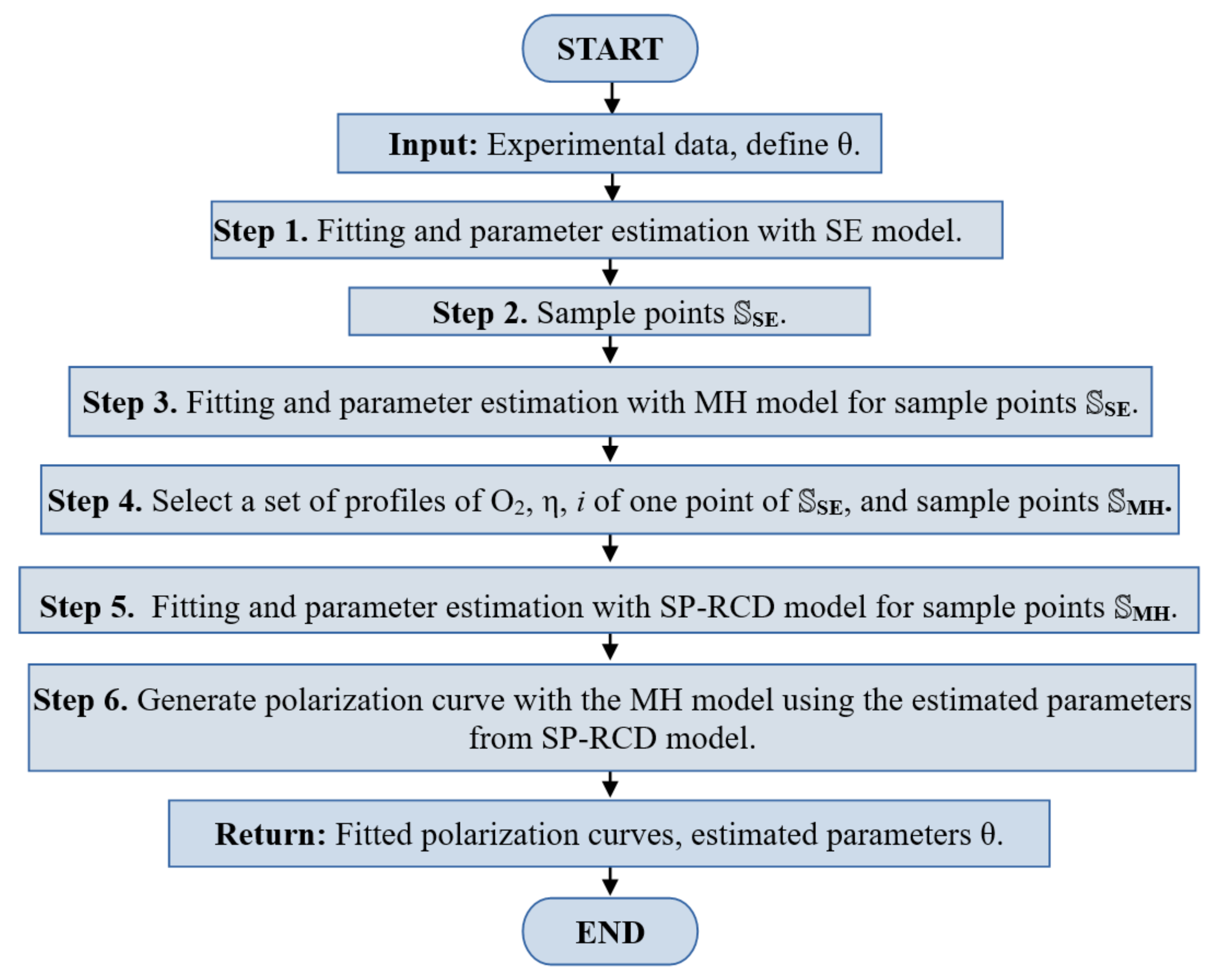
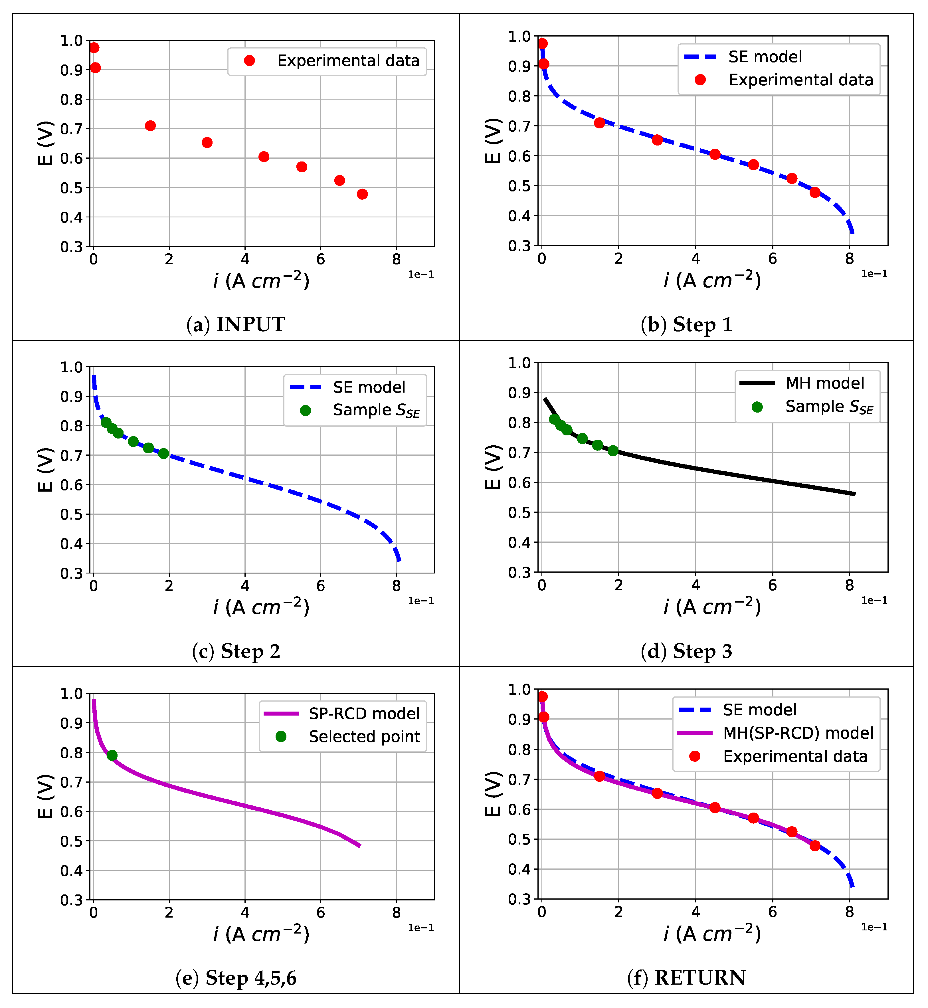
The algorithm begins with an experimental data set of a polarization curve and returns a set of estimated parameters and the fitting of the polarization curve, following steps of the scheme in Figure 4. In this initial step, it is necessary to declare the set of parameters $\overrightarrow{\theta }=\{{\overrightarrow{\theta }}_{SE},{\overrightarrow{\theta }}_{MH},{\overrightarrow{\theta }}_{RCD}\}$ to be estimated. Using the semi-empirical model, we obtained a complete polarization curve, including the concentration losses region. The SE-parameter estimation fitted the model’s output to the experimental data, providing the first set of estimated parameters ${\overrightarrow{\theta }}_{SE}$. As we explain in Section 2.1, this model is incapable of describing the specific physical properties of the catalyst layer.

The macro-homogeneous model describes the missing characteristics that the semi-empiric model is unable to describe; we propose to use a part of the polarization curve simulated by the semi-empiric model, close to the activation losses region, to sample a set of points, called ${\mathbb{S}}_{\mathbb{SE}}$, which was used to estimate a second set of parameters ${\overrightarrow{\theta }}_{MH}$ from the macro-homogeneous model. 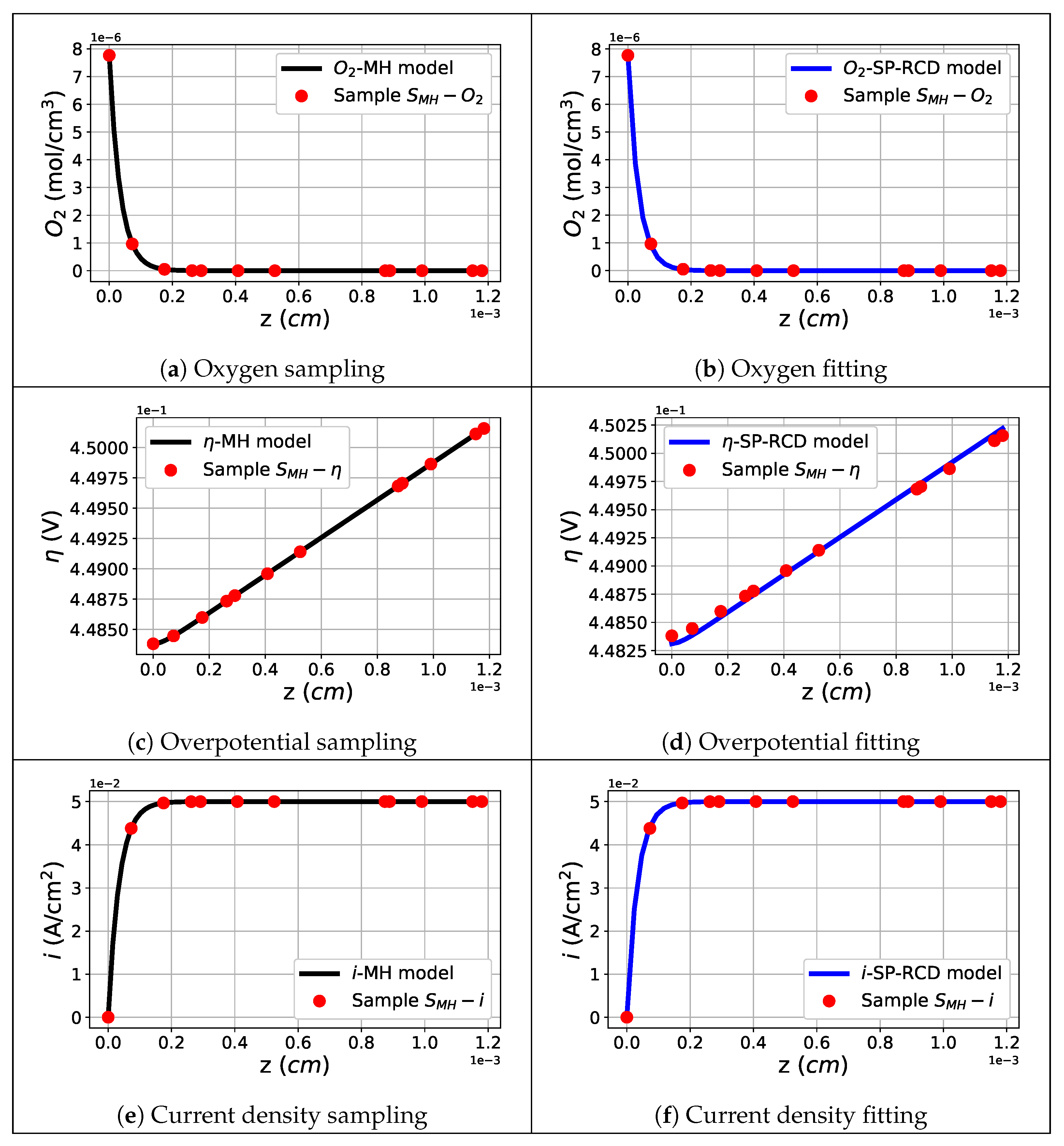It is important to note that in this region, the macro-homogeneous model is well-posed and provides correct solutions, as noted in [13]. With a set of solutions from the macro-homogeneous model corresponding to one point from ${\mathbb{S}}_{\mathbb{SE}}$, the oxygen concentration profiles, overpotentials, and current densities were obtained. It is clear that the estimation of the macro-homogeneous model was correct for the points ${\mathbb{S}}_{\mathbb{SE}}$, but it could not be correct for the complete polarization curve. To improve this, we used the SP-RCD model. Then, we generated a set of sample points named ${\mathbb{S}}_{\mathbb{MH}}$ from the obtained oxygen concentration, overpotential, and current density profiles and used them as data for the parameter estimation with the SP-RCD model. In this step, we re-estimated the previously estimated parameters, ${\overrightarrow{\theta }}_{MH}$, and defined ${\overrightarrow{\theta }}_{RCD}$ as the set of boundary conditions found by the shooting method. Finally, with the new re-estimated parameters ${\overrightarrow{\theta }}_{MH,RCD}=\{{\overrightarrow{\theta }}_{MH},{\overrightarrow{\theta }}_{RCD}\}$, we reproduced the complete polarization curve with the macro-homogeneous model.

This methodology is independent of the parameter estimation problem algorithm and is described as an algorithm that follows the steps below (graphs in Figure 5 and Figure 6), which should be followed in the same way as the methodology steps:

• INPUT: Discrete experimental polarization curve. Define the set of parameters to estimate by each model $\overrightarrow{\theta }=\{{\overrightarrow{\theta }}_{SE},{\overrightarrow{\theta }}_{MH},{\overrightarrow{\theta }}_{RCD}\}$; see Figure 5—INPUT. In this work, we defined the following set of parameters for the estimation: ${\overrightarrow{\theta }}_{SE}=$$\{{\xi }_1$, ${\xi }_3$, ${\xi }_4$, $R_C$, B, $\psi$, A, $L_c$, $J_{max}$}, ${\overrightarrow{\theta }}_{MH}=\{m_{pt},p_{pt},{ϵ}_c\}$, and ${\overrightarrow{\theta }}_{RCD}=\{O_2\left(0\right)$,$\eta \left(0\right)$, $\eta \left(l_c\right)\}$.
• Step 1. We used the semi-empirical model to fit the experimental polarization curve, as shown in Figure 5—Step 1. With this fit, the first set of estimated parameters, ${\overrightarrow{\theta }}_{SE}$, was obtained. More information on the detailed estimation method and its implementation can be found in [34].
• Step 2. We sampled a set of $N_1$ points, named ${\mathbb{S}}_{\mathbb{SE}}$, of the polarization curve fitted by the semi-empirical model in the zone of activation losses, as shown by the green points in Figure 5—Step 2; the example uses $N_1=6$.
• Step 3. We fit the macro-homogeneous model to the sampled points, ${\mathbb{S}}_{\mathbb{SE}}$, as shown by the black line in Figure 5—Step 3; more information on numerical methods to solve the model can be found in [13]. A first approximation of the selected parameters of the MH model ${\overrightarrow{\theta }}_{MH}$ was obtained, as well as the oxygen concentration, overpotential, and current density profiles.
• Step 4. We selected one point (green point in Figure 5—Step 4); used the associated set of profiles obtained by the macro-homogeneous model for oxygen concentration, overpotential, and current density; and sampled $N_2$ points from these profiles, ${\mathbb{S}}_{\mathbb{MH}}$. The sampled points from the profiles are shown in Figure 6a,c,e. In this example, we used $N_2=12$.
• Step 5. We fit the SP-RCD model to the sampled points ${\mathbb{S}}_{\mathbb{MH}}$; then, we obtained estimated parameters ${\overrightarrow{\theta }}_{MH,RCD}=\{{\overrightarrow{\theta }}_{MH},{\overrightarrow{\theta }}_{RCD}\}$. In this process, a second and more precise approximation of the oxygen concentration, overpotential, and current density profiles was obtained, as shown in Figure 6b,d,f. The model was solved using a non-linear finite element formulation with an adaptive Shishkin mesh. Details of the implementation of the SP-RCD model are presented in [41].
• Step 6. We generated the polarization curve by feeding the MH model with the set of estimated parameters ${\overrightarrow{\theta }}_{MH,RCD}=\{{\overrightarrow{\theta }}_{MH},{\overrightarrow{\theta }}_{RCD}\}$ using the SP-RCD, as shown by the magenta continuous line in Figure 5—Step 6.
• RETURN. The estimated set, $\overrightarrow{\theta }$, and the simulated polarization curves were obtained by the semi-empirical and macro-homogeneous models using the estimated parameters from the SP-RCD model.

The proposed methodology is a self-validating strategy as the principal objective of the coupling of the three mathematical models is to generate simulated polarization curves to describe the experimental data of a PEMFC.

5. Results

To validate the proposal, we used two experimental datasets of PEMFC. General information about the reference initial experimental PEMFC can be found in [45]; the authors used Nafion${}^{\circledR }$ 117 with humidified air and prototech-brand electrodes (20 wt. % Pt) onto which they sputtered platinum with an equivalent thickness of 50 nm, corresponding to a total Pt loading of 0.45 mg/cm${}^2$. Complementary base operating conditions used by [12,13] are presented in

Table 4. Parameter values used in the baseline calculation, taken from [12,13].

Base Parameters
Dataset 1 [12]
$N_{cell}=1$	$A_s=112\times {10}^4$ (cm g${}^{-1}$)
R = 8.315 (JK${}^{-1}$ mol${}^{-1}$	${\alpha }_a=0.5$
F = 96485 (C mol${}^{-1}$)	${\alpha }_c=1$
$P_{O_2}=0.21$ (atm)	$\%Pt=0.2$
$T=308$ (K)	$E_{nernst}=1.23$ (V)
$C_{O_2}^{ref}=1.2\times {10}^{-6}$ (mol cm${}^{-3}$)	${ϵ}_g=0.3$
$l_c=1.18\times {10}^{-3}$ (cm)	$L_{g,c}=0$
$R_{ohm}=0.47$ (V)	${\sigma }_S=7.27$ (S cm${}^{-1}$)
$D_{O_2,N}=1.844\times {10}^{-6}$ (cm${}^2$ s${}^{-1}$)	${\sigma }_N=0.17$ (S cm${}^{-1}$)
$D_{O_2,W}=3.032\times {10}^{-5}$ (cm${}^2$ s${}^{-1}$)	${\rho }_C=2.0$ (g cm${}^{-3}$)
$l_{GDL}=200\times {10}^{-4}$ cm	$D_{O_2,GDL}=4.792\times {10}^{-3}$ (cm${}^2$ s${}^{-1}$)
$i_0^{ref}={10}^{3.507-4001/T}$	${ϵ}_c=0.33$
$m_{Pt}=0.332$ (mg cm${}^{-2}$)	${\rho }_{Pt}=21.5$ (g cm${}^{-3}$)
$R{H}_c=R{H}_a=1$	$P_{H_2}=1$ (atm)
$K_{O_2}=\frac{1}{RT}exp\left(-\frac{666}{T}+14.1\right)$	$D_{O_2,gdl}^{eff}=D_{O_2,GDL}{ϵ}_{GDL}^{\frac{3}{2}}$
$O_2\left(0\right)=\frac{1}{K_{O_2}}\left(\frac{P_{O_2}}{RT}-\frac{I_{\delta }{l}_{GDL}}{nF{D}_{O_2,gdl}^{eff}}\right)$
Dataset 2 [13]
$N_{cell}=1$	$R_{ohm}=0.225$ (V)
R = 8.315 (JK${}^{-1}$ mol${}^{-1}$)	${\alpha }_a=0.5$
F = 96485 (C mol${}^{-1}$)	${\alpha }_c=1$
$P=5$ (atm)	${\sigma }_N=0.17$ (S cm${}^{-1}$)
$T=353.15$ (K)	${\sigma }_S=7.27$ (S cm${}^{-1}$)
$C_{O_2}^{ref}=1.2\times {10}^{-6}$ (mol cm${}^{-3}$)	$x_{O_2}=0.21$
$l_c=50$ ($\mu$m)	$L_{g,c}=0.1$
$l_{GDL}=-$	$L_{m,c}=0.4$
$D_{O_2,W}=9.19\times {10}^{-5}$ (cm${}^2$ s${}^{-1}$)	${\rho }_C=1.8$ (g cm${}^{-3}$)
$m_C=4.5$ (mg cm${}^{-2}$)	$E_{nernst}=$ Eq. in ref. [13]
$m_{Pt}=0.35$ (mg cm${}^{-2}$)	${\rho }_{Pt}=21.4$ (g cm${}^{-3}$)
${ϵ}_c=0.4$	$P_{H_2}=5$ (atm)
f = Eq. in Table 3	$A_s$ = Eq. in Table 3
$i_0=$ Eq. in Table 3

.

The optimization algorithm to minimize $SSE\left(\overrightarrow{\theta }\right)$ is an Estimation of the Distribution Algorithm (EDA) named the Univariate Marginal Distribution Algorithm with Gaussian models (UMDA${}^G$) [46,47,48,49,50,51]. It is a stochastic algorithm that computes, in each iteration, the l-dimensional joint probability function, factored as a product of l univariate and independent probability functions. This probability function evolves until a stopping criterion is reached. Details of this algorithm and its implementation are shown in [34,51]. The UMDA${}^G$ uses a population of 200 individuals and 1000 generations with a tolerance of $1\times {10}^{-7}$, for the semi-empirical model. For the macro-homogeneous and the SP-RCD models, it uses a population of 100 individuals and 500 generations with a tolerance of $1\times {10}^{-7}.$ In the context of evolutionary algorithms, the number of individuals in the population is usually considered dependent on the number of parameters to estimate. Thus, for the semi-empirical model, we needed to estimate nine parameters; for the macro-homogeneous model, we needed to estimate three parameters; and for the SP-RCD model, we re-estimated six parameters used in the macro-homogeneous model. Then, the search space for the semi-empirical model should have included more individuals to reach an adequate approximation; meanwhile, the other two models required fewer individuals.

5.1. Dataset 1

We carried out simulations with Dataset 1 (Table 4) and selected 8 points of the polarization curve, which was necessary to obtain the profile of the curvature of the reported polarization curve in [12]. For the semi-empirical model, we selected the set of parameters ${\overrightarrow{\theta }}_{SE}=\{{\xi }_1$, ${\xi }_3$, ${\xi }_4$, $R_C$, B, $\psi$, A, $L_c$, $J_{max}$}. The search space to fit the semi-empirical model with upper and lower bounds is presented in

Table 5. Upper and lower bounds for parameter estimation for the semi-empirical model.

	${\mathit{\xi }}_1$	${\mathit{\xi }}_3$	${\mathit{\xi }}_4$	${\mathit{R}}_{\mathit{C}}$	B	$\mathit{\psi }$	A	${\mathit{L}}_{\mathit{c}}$	${\mathit{I}}_{\mathit{max}}$
${\mathrm{Lim}}_{inf}$	−0.952	7.04 × 10${}^{-5}$	−1.98 × 10${}^{-4}$	0.0001	0.016	14	20	110 × 10${}^{-4}$	0.70
${\mathrm{Lim}}_{sup}$	−0.794	1.50 × 10${}^{-4}$	−0.488 × 10${}^{-4}$	0.0009	0.5	23.5	61.5	190 × 10${}^{-4}$	0.85

. These values are based on previous research [2,23,30,34,37].

With the UMDA${}^G$, we obtained the estimated parameters for the set ${\overrightarrow{\theta }}_{SE}$, as presented in

Table 6. Parameter estimation for the semi-empirical model.

Parameters ${\overrightarrow{\mathit{\theta }}}_{\mathit{SE}}$	Dataset 1	Dataset 2
${\xi }_1$	−0.8928	−0.8973
${\xi }_3$	$8.757\times {10}^{-5}$	$1.147\times {10}^{-4}$
${\xi }_4$	$-1.437\times {10}^{-4}$	$-1.812\times {10}^{-4}$
$R_C$ ( $\Omega$ )	4.0814$\times {10}^{-4}$	6.458$\times {10}^{-4}$
B (V)	4.417$\times {10}^{-2}$	0.2201
$\psi$	21.108	20.866
A (cm${}^2$)	60.489	60.499
$L_c$($\mu$m)	126.5	148.4
$I_{max}$ ($Ac{m}^2$)	0.8088	1.6921
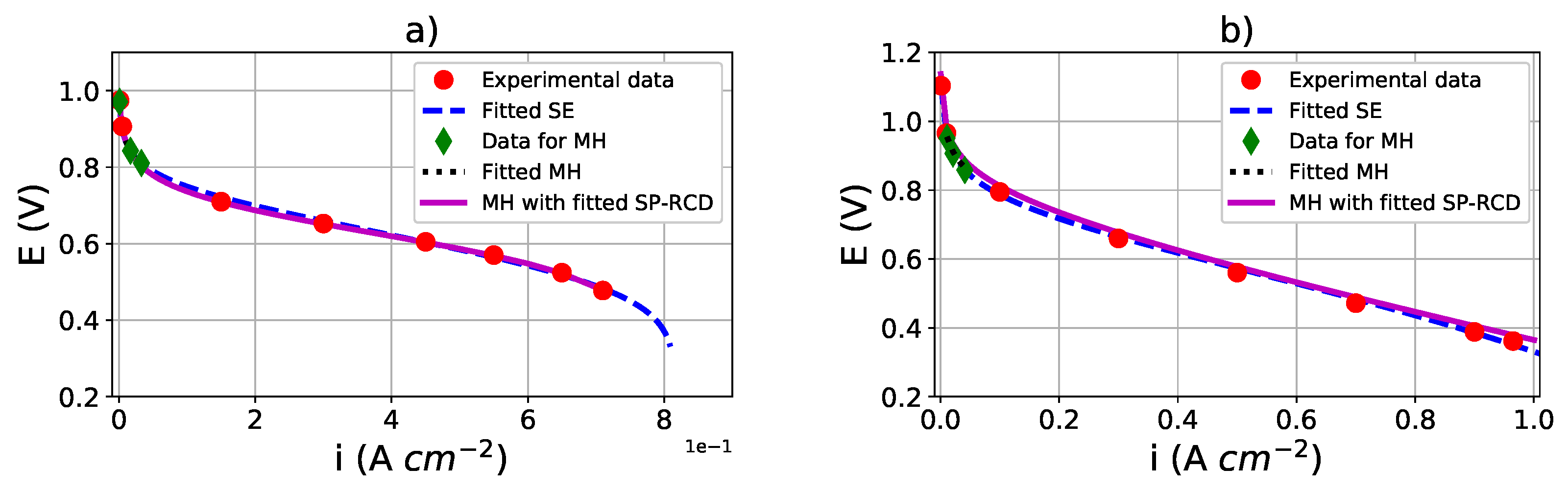
SSE	3.2654$\times {10}^{-4}$	4.941$\times {10}^{-4}$

—Dataset 1, and we generated the simulated initial polarization curve ${\Gamma }_{SE}$, as shown by the dashed blue line in Figure 7a. Next, we sampled three points on ${\Gamma }_{SE}$ to obtain ${\mathbb{S}}_{\mathbb{SE}}$ into the activation losses region, as shown by the green points in Figure 7a, and we used them to obtain the set of estimated parameters ${\overrightarrow{\theta }}_{MH}=\{m_{pt},p_{pt},{ϵ}_c\}$ with the macro-homogeneous model using the search space presented in

Table 7. Upper and lower bounds for parameter estimation for the macro-homogeneous model.

	Dataset 1			Dataset 2
	$m_{pt}$	$p_{pt}$	${ϵ}_c$	$m_{pt}$	$p_{pt}$	${ϵ}_c$
Lim${}_{inf}$	0.2	21	0.31	0.3	18	0.3
Lim${}_{sup}$	0.4	22	0.35	0.4	22	0.5

, based on [12,13,14]; the results are reported in

Table 8. Parameter estimation for the macro-homogeneous and SP-RCD models. ${}^a$ = approximation with the shooting method.

Parameters		Dataset 1			Dataset 2
${\overrightarrow{\theta }}_{MH,RCD}$		Reported [12]	MH	SP-RCD	Reported [13]	MH	SP-RCD
	$m_{Pt}$	0.332	0.3999	0.33063	0.35	0.3009	0.3418
${\overrightarrow{\theta }}_{MH}$	${\rho }_{Pt}$	21.5	21.726	21.8183	21.4	21.997	21.378
	${\epsilon }_g$	0.33	0.3499	0.33354	0.4	0.3000	0.3001
	$O_2\left(0\right)$	-	${}^a$3.9 $\times {10}^{-13}$	7.1 $\times {10}^{-13}$	-	${}^a$2.424 $\times {10}^{-13}$	2.7 $\times {10}^{-13}$
${\overrightarrow{\theta }}_{RCD}$	$\eta \left(0\right)$	-	${}^a$0.44836	0.44838	-	${}^a$0.2997	0.29973
	$\eta \left(l_c\right)$	-	${}^a$0.45016	0.45015	-	${}^a$0.3021	0.30213
SSE	-	-	2.626 $\times {10}^{-4}$	7.156 $\times {10}^{-8}$	-	8.151 $\times {10}^{-5}$	2.434 $\times {10}^{-4}$

—Dataset 1, in which we also present the estimated boundary conditions obtained by a shooting method.

With the results of the macro-homogeneous model, we selected information from the oxygen concentration, overpotential, and current density profiles corresponding to $I_{\delta }=0.05$ Acm${}^{-2}$; we sampled $N_2=10$ uniform points on the profiles and carried out a parameter estimation with the SP-RCD model using the set of parameters ${\overrightarrow{\theta }}_{MH,RCD}$ with ${\overrightarrow{\theta }}_{RCD}=\{O_2\left(0\right),\eta \left(0\right),\eta \left(l_c\right)\}$; the search limits were obtained by perturbing 5% of the estimated values reached with the shooting method in the previous step using the macro-homogeneous model. In Table 8—Dataset 1, we show the estimated values compared to those reported in the literature and to the previously estimated values from the macro-homogeneous model. In Figure 7a, the continuous magenta line represents the simulated polarization curve generated with the macro-homogeneous model using the estimated parameters of the SP-RCD model; the simulated polarization curves are similar and closer together, producing self-validating results.

5.2. Dataset 2

A second dataset was used with the baseline parameters in Table 4—Dataset 2; we selected eight points of the experimental polarization curve, and the reported experimental data are presented in [13]. For the semi-empirical model, we used the same set of parameters and the search space in Table 2, except for $I_{max}$; we increased the interval to $[0.7,1.8]$ following the reported values in [18] to preserve the profile of the experimental polarization curve. The estimations are presented in Table 6—Dataset 2. In Figure 7b, the dashed blue line represents the simulated polarization curve ${\Gamma }_{SE,2}$ obtained from the semi-empirical model. We sampled $N_1=3$ points on ${\Gamma }_{SE,2}$ to obtain ${\mathbb{S}}_{\mathbb{SE}}$, as shown by the green points in Figure 7b. For the macro-homogeneous model, we estimated the set of parameters ${\overrightarrow{\theta }}_{MH}=\{m_{pt},p_{pt},{ϵ}_c\}$, similar to that for Dataset 1. We report the estimated parameters in Table 8—Dataset 2. For parameter estimation with the SP-RCD model, we selected the profiles of oxygen concentration, overpotential, and current density corresponding to $I_{\delta }=0.21$ Acm${}^{-2}$; we sampled $N_2=10$ uniform points on the profiles, overpotential, and current density. In the estimation process, we included ${\overrightarrow{\theta }}_{RCD}=\{O_2\left(0\right)$,$\eta \left(0\right)$, $\eta \left(l_c\right)\}$. We compared the estimated values with those reported in [13], and with estimated values from the macro-homogeneous model in Table 8—Dataset 2. We present the simulated polarization curve generated by the macro-homogeneous model using the estimated values with SP-RCD in Figure 7b, as shown by the continuous magenta line.

The results of the numerical experiments in this work provide us with coherent and similar results to those obtained in previous works [12,13,34] (see Table 6 and Table 8). The simulated polarization curves with the semi-empirical or macro-homogeneous models using the estimated parameters of the SP-RCD are similar and close together, showing that our methodology is adequate to describe PEMFC performances.

6. Conclusions

In this article, we described a proposal of a self-validating methodology using three different mathematical models: semi-empirical (SE), macro-homogeneous (MH), and singularly perturbed reaction–convection–diffusion (SP-RCD). The set of linked parameter estimation problems, solved by the UMDA${}^G$, uses the benefits and advantages of each model to circumvent the disadvantages of the others. With the proposal in this work, it is possible to analyze the performance of a PEMFC, from the operational and construction parameters to the structural and composition parameters in the catalyst layer. The semi-empirical model describes the operational and construction parameters, such as temperature, pressure, and membrane properties; meanwhile, the macro-homogeneous and the SP-RCD models are useful to determine the composition parameters, such as platinum mass loading $m_{Pt}$. The coupling of the models serves to take advantage of the polarization curve region that is better fitted by each one; for instance, the SE model reproduces the catalyst activation region; then, the MH takes the SE output to produce a gross approximation of the boundary conditions of the concentration profiles and a set of parameters. The actual boundary conditions and parameters are re-estimated with the SP-RCD model, producing more precise solutions. This last precise solution is inputted into the MH model to obtain a correction of the polarization curve.

The results are comparable with those reported in the literature; the simulated polarization curves of the semi-empirical and macro-homogeneous models obtained using the estimated parameters of the SP-RCD are similar and close together, validating the approximations between the models. The power of the method is to estimate parameters that are difficult or impossible to measure, starting from experimental information. Nevertheless, once we estimate the parameters that reproduce the experimental data, one can change a few parameters to describe the performance of a different design. Furthermore, one can use the model to optimize the performance of a PEMFC by testing parameters in a physically plausible interval of values. This strategy equips the practitioners with complementary information about parameters that are difficult to measure experimentally in a laboratory and increases the confidence of the estimated parameters that consistently reproduce the experimental data. Future work contemplates the optimization of the parameters. Notice that a first step to optimizing a PEMFC is to have a reliable numerical simulation that reproduces the actual polarization curve and concentration species profiles. Once the adequate parameters for the models have been determined by means of the proposed methodology, it is possible to vary any parameter, not only the estimated ones, to find an optimized value for improving the cell performance or cost. For example, it could be the platinum mass loading $m_{Pt}$, for which optimization could reduce the cost while maintaining the performance of the original design, or the operational parameters to increase the electricity generation with the same design.

References

1. Wang, J.; Wang, H.; Fan, Y. Techno-Economic Challenges of Fuel Cell Commercialization. Engineering 2018, 4, 352–360. [Google Scholar] [CrossRef]
2. Outeiro, M.; Chibante, R.; Carvalho, A.; de Almeida, A. A parameter optimized model of a Proton Exchange Membrane fuel cell including temperature effects. J. Power Sources 2008, 185, 952–960. [Google Scholar] [CrossRef]
3. Sun, S.; Su, Y.; Yin, C.; Jermsittiparsert, K. Optimal parameters estimation of PEMFCs model using Converged Moth Search Algorithm. Energy Rep. 2020, 6, 1501–1509. [Google Scholar] [CrossRef]
4. Zhang, J.; Sanderson, A. JADE: Adaptive differential evolution with optional external archive. IEEE Trans. Evol. Comput. 2009, 13, 945–958. [Google Scholar] [CrossRef]
5. Ohenoja, M.; Leiviskä, K. Validation of genetic algorithm results in a fuel cell model. Int. J. Hydrogen. Energy 2010, 35, 12618–12625. [Google Scholar] [CrossRef]
6. Lu, D.; Djilali, N.; Berning, T. Three-dimensional computational analysis of transport phenomena in a PEM fuel cell. J. Power Sources 2002, 106, 284–294. [Google Scholar]
7. Berning, T.; Djilali, N. A 3D, Multiphase, Multicomponent Model of the Cathode and Anode of a PEM Fuel Cell. J. Electrochem. Soc. 2003, 150, A1589. [Google Scholar] [CrossRef]
8. Berning, T.; Djilali, N. Three-dimensional computational analysis of transport phenomena in a PEM fuel cell a parametric study. J. Power Sources 2003, 124, 440–452. [Google Scholar] [CrossRef]
9. Tiedemann, W.; Newman, J. Maximum Effective Capacity in an Ohmically Limited Porous Electrode. J. Electrochem. Soc. 1975, 122, 1482–1485. [Google Scholar] [CrossRef]
10. Marr, C.; Li, X. Composition and performance modelling of catalyst layer in a proton exchange membrane fuel cell. J. Power Sources 1999, 77, 17–27. [Google Scholar] [CrossRef]
11. You, L.; Liu, H. A parametric study of the cathode catalyst layer of PEM fuel cells using a pseudo-homogeneous model. Int. J. Hydrogen Energy 2001, 26, 991–999. [Google Scholar] [CrossRef]
12. Song, D.; Wang, Q.; Liu, Z.; Navessin, T.; Eikerling, M.; Holdcroft, S. Numerical optimization study of the catalyst layer of PEM fuel cell cathode. J. Power Sources 2004, 126, 104–111. [Google Scholar] [CrossRef]
13. Khajeh-Hosseini-Dalasm, N.; Kermani, M.; Moghaddam, D.G.; Stockie, J. A parametric study of cathode catalyst layer structural parameters on the performance of a PEM fuel cell. Int. J. Hydrogen Energy 2010, 35, 2417–2427. [Google Scholar] [CrossRef]
14. Heidary, H.; Jafar Kermani, M.; Khajeh-Hosseini-Dalasm, N. Performance analysis of PEM fuel cells cathode catalyst layer at various operating conditions. Int. J. Hydrogen Energy 2016, 41, 22274–22284. [Google Scholar] [CrossRef]
15. Secanell, M.; Karan, K.; Suleman, A.; Djilali, N. Multi-variable optimization of PEMFC cathodes using an agglomerate model. Electrochim. Acta 2007, 52, 6318–6337. [Google Scholar] [CrossRef]
16. Shah, A.; Kim, G.S.; Sui, P.; Harvey, D. Transient non-isothermal model of a polymer electrolyte fuel cell. J. Power Sources 2007, 163, 793–806. [Google Scholar] [CrossRef]
17. Wang, G.; Mukherjee, P.P.; Wang, C.Y. Optimization of polymer electrolyte fuel cell cathode catalyst layers via direct numerical simulation modeling. Electrochim. Acta 2007, 52, 6367–6377. [Google Scholar] [CrossRef]
18. Outeiro, M.T.; Chibante, R.; Carvalho, A.S.; de Almeida, A.T. A new parameter extraction method for accurate modeling of PEM fuel cells. Int. J. Od Energy Res. 2009, 33, 978–988. [Google Scholar] [CrossRef]
19. Zhang, L.; Wang, N. An adaptive RNA genetic algorithm for modeling of proton exchange membrane fuel cells. Int. J. Hydrogen. Energy 2013, 38, 219–228. [Google Scholar] [CrossRef]
20. Gong, Z.; Liu, C.; Teo, K.L.; Sun, J. Distributionally robust parameter identification of a time-delay dynamical system with stochastic measurements. Appl. Math. Model. 2019, 69, 685–695. [Google Scholar] [CrossRef]
21. Shen, B.; Liu, C.; Ye, J.; Feng, E.; Xiu, Z. Parameter identification and optimization algorithm in microbial continuous culture. Appl. Math. Model. 2012, 36, 585–595. [Google Scholar] [CrossRef]
22. Ye, M.; Wang, X.; Xu, Y. Parameter identification for proton exchange membrane fuel cell model using particle swarm optimization. Int. J. Hydrogen Energy 2009, 34, 981–989. [Google Scholar] [CrossRef]
23. Askarzadeh, A.; Rezazadeh, A. Artificial immune system-based parameter extraction of proton exchange membrane fuel cell. Int. J. Electr. Power Energy Syst. 2011, 33, 933–938. [Google Scholar] [CrossRef]
24. Mo, Z.J.; Zhu, X.J.; Wei, L.Y.; Cao, G.Y. Parameter optimization for a PEMFC model with a hybrid genetic algorithm. Int. J. Energy Res. 2006, 20, 585–597. [Google Scholar] [CrossRef]
25. Cheng, J.; Zhang, G. Parameter fitting of PEMFC models based on adaptive differential evolution. Int. J. Electr. Power Energy Syst. 2014, 62, 189–198. [Google Scholar] [CrossRef]
26. Turgut, O.E.; Coban, M.T. Optimal proton exchange membrane fuel cell modelling based on hybrid Teaching Learning Based Optimization-Differential Evolution algorithm. Ain Shams Eng. J. 2016, 7, 347–360. [Google Scholar] [CrossRef]
27. Askarzadeh, A.; Rezazadeh, A. Optimization of PEMFC model parameters with a modified particle swarm optimization. Int. J. Energy Res. 2011, 35, 1258–1265. [Google Scholar] [CrossRef]
28. Jayakumar, A.; Ramos, M.; Al-Jumaily, A. A Novel fuzzy schema to control the temperature and humidification of PEM fuel cell system. Int. Conf. Fuel Cell Sci. Eng. Technol. 2015, 56611, V001T06A005. [Google Scholar] [CrossRef]
29. Askarzadeh, A.; Rezazadeh, A. A grouping-based global harmony search algorithm for modeling of proton exchange membrane fuel cell. Int. J. Hydrogen Energy 2011, 36, 5047–5053. [Google Scholar] [CrossRef]
30. Xu, S.; Wang, Y.; Wang, Z. Parameter estimation of proton exchange membrane fuel cells using eagle strategy based on JAYA algorithm and Nelder-Mead simplex method. Energy 2019, 173, 457–467. [Google Scholar] [CrossRef]
31. Saremi, S.; Mirjalili, S.; Lewis, A. Grasshopper Optimisation Algorithm: Theory and application. Adv. Eng. Softw. 2017, 105, 30–47. [Google Scholar] [CrossRef] [Green Version]
32. Mirjalili, S.; Gandomi, A.H.; Mirjalili, S.Z.; Saremi, S.; Faris, H.; Mirjalili, S.M. Salp Swarm Algorithm: A bio-inspired optimizer for engineering design problems. Adv. Eng. Softw. 2017, 114, 163–191. [Google Scholar] [CrossRef]
33. Ben Messaoud, R.; Midouni, A.; Hajji, S. PEM fuel cell model parameters extraction based on moth-flame optimization. Chem. Eng. Sci. 2021, 229, 116100. [Google Scholar] [CrossRef]
34. Blanco-Cocom, L.; Botello-Rionda, S.; Ordoñez, L.; Valdez, S.I. Robust parameter estimation of a PEMFC via optimization based on probabilistic model building. Math. Comput. Simul. 2021, 185, 218–237. [Google Scholar] [CrossRef]
35. Zhang, J. PEM Fuel Cell Electrocatalysts and Catalyst Layers: Fundamentals and Applications; Springer: London, UK, 2008; Volume 1. [Google Scholar] [CrossRef]
36. Berger, C. Handbook of Fuel Cell Technology; Prentice Hall: Engelwood Cliffs, NJ, USA, 1968. [Google Scholar]
37. Mann, R.F.; Amphlett, J.C.; Hooper, M.A.; Jensen, H.M.; Peppley, B.A.; Roberge, P.R. Development and application of a generalised steady-state electrochemical model for a PEM fuel cell. J. Power Sources 2000, 86, 173–180. [Google Scholar] [CrossRef]
38. Farrell, P.; Hegarty, A.; Miller, J.; O’Riordan, E.; Shishkin, G. Robust Computational Techniques for Boundary Layers; CRC Press: Boca Raton, FL, USA, 2000. [Google Scholar]
39. Roos, H.; Stynes, M.; Tobiska, L. Robust Numerical Methods for Singularly Perturbed Differential Equations; Springer: Berlin/Heidelberg, Germany, 2008. [Google Scholar]
40. Kierzenka, J.A.; Shampine, L.F. A BVP solver that controls residual and error. J. Numer. Anal. Ind. Appl. Math. 2008, 3, 27–41. [Google Scholar]
41. Blanco-Cocom, L.; Botello-Rionda, S.; Ordoñez, L.; Valdez, S.I. A reaction–convection–diffusion model for PEM fuel cells. Finite Elem. Anal. Des. 2022, 201, 103703. [Google Scholar] [CrossRef]
42. Carnes, B.; Djilali, N. Systematic parameter estimation for PEM fuel cell models. J. Power Sources 2005, 144, 83–93. [Google Scholar] [CrossRef]
43. Scott, K.; Argyropoulos, P. A one dimensional model of a methanol fuel cell anode. J. Power Sources 2004, 137, 228–238. [Google Scholar] [CrossRef]
44. Yang, B.; Wang, J.; Yu, L.; Shu, H.; Yu, T.; Zhang, X.; Yao, W.; Sun, L. A critical survey on proton exchange membrane fuel cell parameter estimation using meta-heuristic algorithms. J. Clean. Prod. 2020, 265, 121660. [Google Scholar] [CrossRef]
45. Ticianelli, E.A. Methods to Advance Technology of Proton Exchange Membrane Fuel Cells. J. Electrochem. Soc. 1988, 135, 2209. [Google Scholar] [CrossRef]
46. Larrañaga, P.; Lozano, J.A. Estimation of Distribution Algorithms: A New Tool for Evolutionary Computation; Kluwer Academic Publishers: Philip Drive Norwell, MA, USA, 2002; Volume 1. [Google Scholar]
47. Mühlenbein, H. The equation for response to selection and its use for prediction. Evol. Comput. 1998, 5, 303–346. [Google Scholar] [CrossRef]
48. Syswerda, G. Simulated crossover in genetic algorithms. Found. Genet. Algorithms 1993, 2, 239–255. [Google Scholar]
49. Eshelman, L.J.; Schaffer, J.D. Productive recombination and propagating and preserving schemata. Found. Genet. Algorithms 1993, 3, 299–314. [Google Scholar]
50. Mühlenbein, H.; Voigt, H.M. Gene Pool Recombination in Genetic Algorithms; Springer: Boston, MA, USA, 1996; pp. 53–62. [Google Scholar]
51. Valdez Peña, S.; Hernández-Aguirre, A.; Botello, S. Approximating the search distribution to the selection distribution in EDAs. In Proceedings of the 11th Annual Conference on Genetic and Evolutionary Computation, Montreal, QC, Canada, 8–12 July 2009; pp. 461–468. [Google Scholar] [CrossRef]
Figure 1. Basic structure of a proton exchange membrane fuel cell.
Energies 15 00885 g001
Figure 2. Polarization curve of a PEM fuel cell; additional information in [35]. V * = Voltage loss caused by mixed potential and crossover.
Energies 15 00885 g002
Figure 3. Schematic diagram of the Membrane Electrode Assembly (MEA) in a PEMFC.
Energies 15 00885 g003
Figure 4. Flowchart of the proposed self-validating methodology. This diagram is complemented by Figure 5 and Figure 6.
Energies 15 00885 g004
Figure 5. General steps of the proposed self-validating methodology: (a) INPUT: obtain the set of experimental data and define the corresponding set θ = { θ S E , θ M H , θ R C D } of parameters to estimate in the process; (b) fit the SE model to the experimental data; we obtained θ S E ; (c) sample some points from the SE solution to generate the set, S SE ; (d) use the MH model to fit the points S SE ; we obtained θ M H ; (e) select one point from S SE with its macro-homogeneous solutions to sample point S MH and fit it to the SP-RCD model (in this example, I δ = 0.05 Acm 2 ); we obtained θ M H , R C D , as expanded in Figure 6; (f) RETURN: final polarization curves with the SE and the MH models using the estimated parameters θ M H , R C D .
Energies 15 00885 g005
Figure 6. Steps 4 and 5 of the proposed self-validating methodology: sample points, S MH , from solutions of the MH model for I δ = 0.05 Acm 2 (step 4) and fit them with the SP-RCD model (step 5); in this step, we obtained θ M H , R C D .
Energies 15 00885 g006
Figure 7. Numerical experiments: (a) Dataset 1 [12]; (b) Dataset 2 [13].
Energies 15 00885 g007