Soil State Testing Using Heavy Vehicle Vibrations

Abstract

Changes in the elastic characteristics of the railway subgrade have been determined using nonstop long-term (more than 50 days) train passage seismic observations. We examined the records of the broadband sensitive seismometer TC-120s in the low-frequency band (below 0.1 Hz) to obtain the subgrade response to various train passages and its relaxation after unloading. Analytical models of subgrade deformation by the train are proposed. When comparing models in the experiment, we showed that a lowpass filter (below 0.1 Hz) provides waveforms with parameters determined by the deformation properties of the soil. We carried out statistical processing of 1600 train seismic records and determined parameters characterizing the subgrade reaction to the vibration effects created by trains in the ultra-low-frequency range. Therefore, we can use these parameters to monitor after daily averaging and weekly smoothing. When observing the spring thawing of the soil, we considered the sensitivity of seismic monitoring using heavy vehicle vibrations, particularly changes in the soil state properties under a rise in ambient temperature. The presented observations can be used for seismic monitoring technology at an early stage of hazardous processes in the subgrade.

1. Introduction

Climatic changes and increases in technogenic transport load (e.g., the volume of cargo transportation, train weight, and its speed increase, etc.) lead to the degradation subgrade of the bearing capacity in difficult soil conditions such as permafrost and its thawing, swampy areas, subsidence soils, etc. [1,2].

The operation of the subgrade stability requires constant monitoring of their condition including the base soils. Now, there is a wide range of instrumental survey methods to control the subgrade state [3,4,5,6,7,8,9] including seismic ones (e.g., [10,11,12,13,14,15]), but all of them have three main features that are the main gaps in soil state monitoring:

• Episodic testing (according to the schedule or in emergency situations), continuous observations (monitoring) are not carried out;
• Changes in the subgrade state are detected at stages close to emergency, i.e., not at an early stage of the dangerous phenomenon development; and
• The survey requires a visit to the site and does not practice the subgrade state remote monitoring via cloud platforms, for example, presented in [16,17].

Creating technology that can eliminate these limitations could be the basis of a new phase in security.

The main research questions are:

(i)

to obtain analytical models of soil deformation near the track when exposed to a moving train and coinciding with the experiment;

(ii)

to find the parameters of the seismic record obtained near the railway, by which it is possible to determine the change in the soil state, not critical to the weight of the vehicle, and its speed and suitability for automated processing; and

(iii)

on an experimental example of seasonal changes in soil state, show the sensitivity of the selected parameters for monitoring.

The main goal is to create the basis of new vibro seismic monitoring technology using the moving heavy vehicle influence as a ground probing load.

In this paper, we considered the first results of this technology, which we developed based on the example of assessing the railway subgrade state. The basis of the idea is the use of a modern hardware and methodological complex with a broadband seismometer while using the moving train vibration as a ground probing load. Additionally, we investigated the soil response to vibration loads (soil dynamics) created by passing trains, which cause a deformation and decrease in the soil stress.

The average weight of a cargo train is 6000–8000 tons, the speed is 70–90 km/h, and about a hundred trains pass along the track per day, which characterizes a significant size and constant technogenic load on the soils. It is important that a moving train has a combined effect on the track base: a relatively high-frequency vibrational (above 1–5 Hz, e.g., [18,19,20,21,22,23,24]) and deformation similar to a moving stamp (frequencies below 1 Hz up to periods of 100 s [25,26]). High-frequency oscillations are created by the interaction of wheels and track, and have been studied quite completely (e.g., [27,28,29]) and are the basis for several technologies for surveying the subgrade state (e.g., [23,30,31,32,33]). Low-frequency, and especially ultra-low-frequency (up to periods 100 s), oscillations have been studied only on soil samples and for the vertical component [34,35,36,37] because there were no corresponding observing facilities. Nowadays, appropriate instruments include the broadband seismometers usually used in seismology. Moreover, vibro impact on soils have been studied at the micro level (i.e., when the structural connections between soil particles change). In in situ experiments, the absorption of vibrations of different intensities up to nonlinear phenomena in strong earthquakes was studied [38,39,40].

The subgrade response to low-frequency vibrations generated by the train is determined by its elastic properties. Considering that the additional deformation at the observation site is proportional to the amplitude of vibrations [41], by analyzing the amplitude variations of low-frequency impacts during continuous monitoring, it is possible to determine the change in the subgrade state.

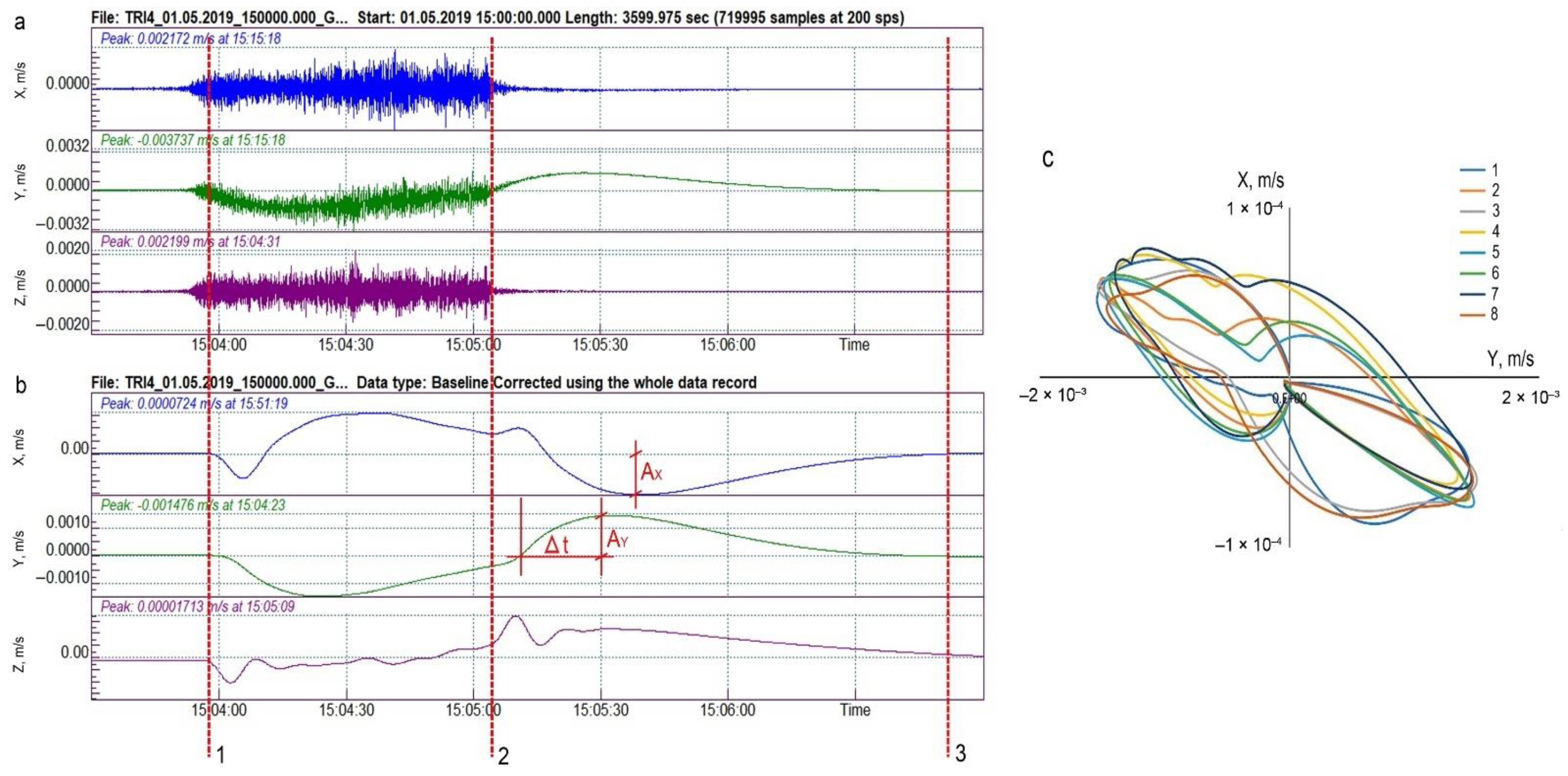
The observation of long-period oscillations created by passing trains was first performed by us in previous studies [25,26,42]. Figure 1 shows the train passage records obtained near the embankment on three orthogonal components $X,Y, Z$ (where X, $Y$ are horizontal components directed along and across the track, respectively, $Z$ is the vertical component). Waveforms are shown in a wide frequency band and after filtering by a lowpass filter below 0.1 Hz. Vertical lines limit the time interval for a train to pass by the sensor. One can see that there is a subgrade reaction to the deforming train load on all components both during its movement and after removing the load (i.e., after train passing (subgrade relaxation)). The waveforms differ for the components. There was a distinct surge of oscillations at the beginning of the train passage on the $Z$-component. On horizontal components, low-frequency waveforms showed a pattern of medium deforming as the load increased, and then when the load was removed, the original subgrade state was restored. This can also be seen in the diagrams of the subgrade site movement (in seismometer installation site) in the horizontal plane during the train passage (Figure 1c), where a kind of hysteresis can be observed. Note that the oscillation amplitude on component $Y$ is an order of magnitude greater than one on X. This fact reflects a greater fixation of the embankment along the path compared to the mobility across the path.

The similarity of long-period waveforms in the horizontal plane, as opposed to that on the $Z$-component, indicates different laws of deformation of the medium. Essentially, we are dealing with a moving heavy stamp and need to understand how deformations change over time at the sensor installation site, which is away from the line of stamp motion. Numerical medium deformation simulation usually involves a quasi-static load and a static picture of the spatial deformation distribution [26], but does not give the desired waveforms. Another possibility is the theoretical consideration of the problem and obtaining analytical solutions. We made such attempts to explain the features of the waveforms of the $Z$-component. We considered the problem of the elastic half-space deformation by a moving load and obtained results corresponding to our experiment [25]. However, no explanation of the features experimentally observed on the horizontal components has been obtained, which is one of the subjects of this article.

Another issue that needs to be studied for continuous monitoring is the problem of the repetitiveness of the impact. When analyzing the waveforms obtained during seismic monitoring, one must be sure that the subgrade state has changed, and not the impact. Given that the weight and speed of the train and quality of the clutch to the tracks differ for trains, it is difficult to expect a good repeatability of the impact on the subgrade for each train in the set. We had an idea to use the stability of the statistical advantage for the impact parameter ensemble of trains for a day, a week or more—this is already hundreds of impacts. Evaluating these statistics and finding the characteristic parameters of waveforms is the second issue discussed in the article.

Finally, another topic discussed in the article is the search for seismic waveform parameters that are informative for detecting changes in the subgrade and are available for automated record processing in the observation point. Then, these parameters can be transmitted during remote continuous monitoring.

The possibility of detecting hazardous processes in soils at an early stage during seismic monitoring using trains was partially discussed by us in a number of works in which the resolution of the technology was assessed and the possibility of detecting non-hazardous flooding [25,26] was experimentally shown. Here, we will touch upon a question for the continuous monitoring problem such as seasonal changes in soils.

2. Materials and Methods

The basis of this work was experimental seismic data to explain the features of which we have attracted the problems known in theoretical mechanics and seismology for the deformation of the medium—the Boussinesq solution [25,43] and the Elsasser model [44].

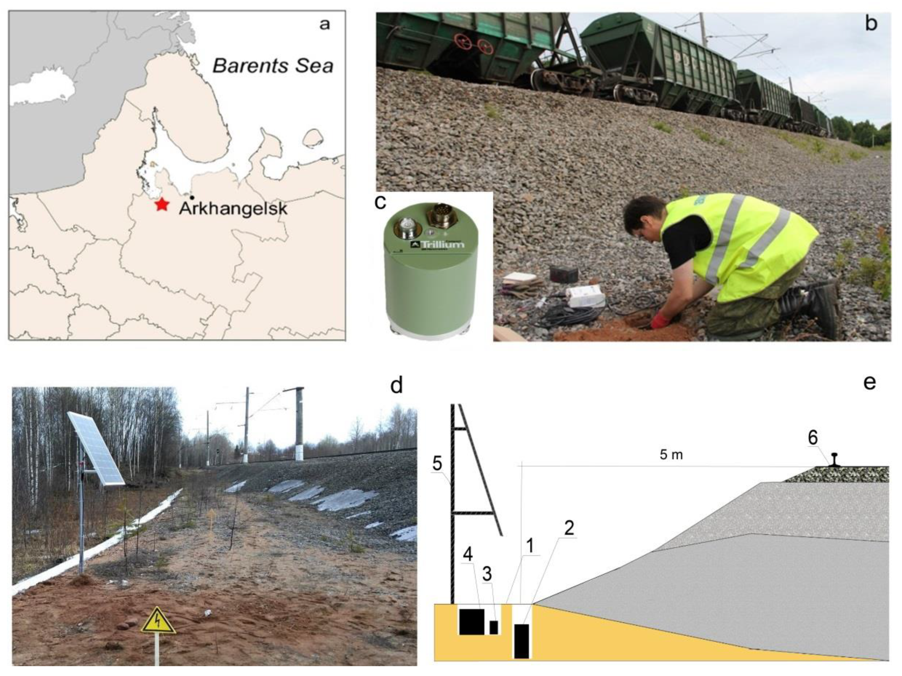
Seismic observations were conducted on the section of the Northern Railway in the Arkhangelsk region, northern Russia (see map Figure 2) in 2017 and 2019. We carried out shallow seismic prospecting to obtain seismic sections and direct observations of oscillations during the train passage. For this purpose, we tested sensors of different types [26], as a result, we selected a seismometer-velocimeter TC-120s (Nanometrics, Ottawa, Canada), which allows for oscillations to be recorded with periods up to 120 s. The sensor was installed at about 5 m from the track at a depth of 80 cm, the power supply was from solar panels, and the data were recorded on the flash memory built into the datalogger (Figure 2). In 2017, we made relatively short-term observations for several days. We registered cargo and passenger trains and single locomotives. The different train types on seismic records are clearly separated by the time duration and by the oscillation amplitude values. This problem is discussed later (Figure 3). The lowest values were single locomotives, the largest were cargo trains, since they are the heaviest, and have about 70 cars on average. In 2019, continuous registration was about 50 days, and signals from 1600 trains were recorded. From 30 to 40 trains were registered daily with the predominant number (almost 90%) being cargo trains. It is significant that observations in 2017 were in dry and hot weather (August), and in 2019 in rainy weather, with melting snow and thawing of soils. We considered this experiment as a full-scale model of changes in the state of the roadbed soils.

When record processing, the seismic vibrations associated with the train passage were picked, first manually, and then by applying the STA/LTA algorithm [45], which is used in seismology to detect events. Then, we performed filtering in the frequency ranges of bandpass filter 2–8 Hz; lowpass filter 0.1 Hz; and bandpass filter 0.1–0.5 Hz, which we used to obtain maximum amplitudes at the beginning of train movement recording. This operation, similar to the previous one, was automated. Below are the results of using a lowpass filter; ones for bandpass filter 2–8 Hz are discussed in the work by [46]. As record parameters, these were adopted that met the requirements:

• Can indicate the medium deformation process;
• Are well repeated for different trains; and
• Simple and univocal identifiable for automated processing.

Requirements 1 and 2 were partially discussed in our previous works [25,26], here, we summarize the experience to understand the soil deformation mechanisms caused by a moving train.

As a result, after applying the lowpass filter, the following parameters for displacement velocity recording were adopted: the amplitude of the first extremum on the vertical component (A_Z), the amplitudes of A_X, A_Y of the subgrade relaxation of the recording after the train passed, the first after crossing the zero line, and Δt—the time from crossing the zero line to the maximum A_Y (see Figure 2).

3. Results

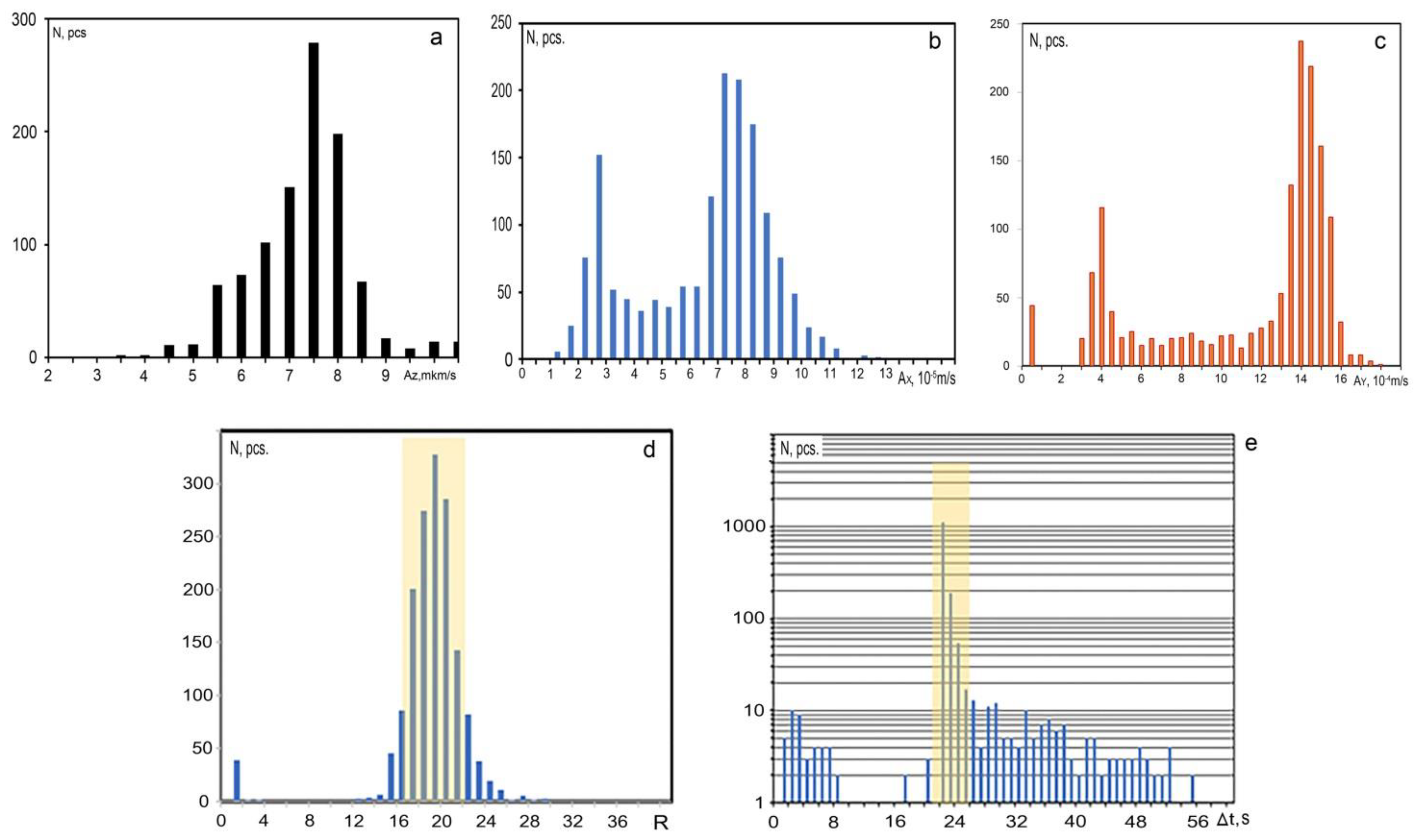
As a result of automated processing, we obtained data arrays of parameters A_Z, A_X, A_Y, and Δt. Given that the trains are different (passenger and cargo) and have different speeds, etc., we conducted descriptive statistics and built histograms of parameter values to identify representative values (Figure 3). In each distribution, there were distinct maxima. Note that there are two maximums on the distributions for A_X and A_Y, which, as we noticed in the process of visual observation, corresponds to different types of trains—lighter passenger and cargo. To exclude the influence of the weight of the train and possibly its speed, we used the parameter R = |A_Y/A_X|. The resulting histogram of R values has one distinct maximum, which reduces the influence of train parameters. To reduce the impact of the train’s characteristics, we excluded the data outside the single-sigma corridor relative to the median value. Note that the calculation of descriptive statistics is a stage of setting up processing, is performed at the beginning of observations, and is not included in the automation algorithm. The resulting arrays of record parameter values are accepted for further analysis. Therefore, we obtained the following statistical values for some of the parameters, as presented in

Table 1. Statistical values for selected parameters characterizing the subgrade reaction to the vibration effects created by trains in the ultra-low-frequency range.

Parameter	Median Value	Single-Sigma Corridor Value
R	18.4	3.7
Δt, s	21.8	8.1
AZ, μm/s	7.5	1.3

.

Analytical models have been proposed to explain the above-mentioned features of the experimental records and to enable the transition from a set of parameters to the assessment of soil dynamics in the ultra-low-frequency range [35,36,37]. Model 1 is the problem of the elastic half-space deformation by a moving load in three directions ($X, Y, Z$). Model 2 is the problem of the elastic layer over a viscous half-space and describes the space–temporal distribution of medium stress in the horizontal plane. We considered direction away from the rails.

Model 1. The experimental data obtained by us constitute the subject of theoretical consideration, which is the basis of the proposed technology. The theoretical problems under consideration are dynamic. However, if we take into account the characteristic size, the rate of load increase, and the speed of propagation of elastic waves, then a good approximation would be a process that passes through many equilibrium states. In other words, theoretical research uses static problems in which time plays the role of a parameter.

In the half-space, there is a subgrade that has the shape of a trapezoid in cross-section; it is essentially a thick plate with beveled edges. The load is applied to the upper plane of the subgrade, and the subgrade in this sense is the object of transferring the load to the surface of the half-space. As a result, we obtained the problem of deformation of the half-space under the action of a system of forces applied to the surface. The half-space is considered linear-elastic, and is accepted to be isotropic, homogeneous, and the loads are vertical. It is important to note that the task was only examined for a sensor located outside the real load application area. The load on the rails was further carried out by the wheelsets. Therefore, the load element is the load from one wheelset. The action of several elementary loads including those distributed over the area is calculated according to the principle of superposition.

To this approximation, deformation of the subgrade is reduced to solving the Boussinesq solution for a homogeneous elastic half-space with a train as a moving force that creates displacements at a given point [25]. Previously, we obtained an analytical solution for the vertical component of the vibration velocity when the train is moving [25]:

$$\frac{dw}{dt}=-\frac{P{V}^{2}t}{4\pi \mu }\left(\frac{3z^2}{R^5}+\frac{2\left(1-\nu \right)}{R^3}\right),$$

(1)

where P is the vertical force; V is the velocity; μ is the shear modulus; ν is the Poisson coefficient; ($x,y,z$) are the coordinates of the sensor point; ($X, Y$) is the point of force load, $X=Vt,$ $Y$ = 0, and

$$R=\sqrt{{(x-X)}^2+{(y-Y)}^2+z^2}.$$

(2)

In Equation (1), the moment t = 0 corresponds to the position when the force is opposite the sensor. If we substitute Vt–l instead of Vt, we obtain a force moving one meter later than the force with Vt. This technique can be used to obtain the result from the simultaneous action of numerous forces, for example, wagons. This was discussed in [25] and it was shown that the wave forms of the first arrivals were determined by the first wheel pair.

Similarly, we obtain:

Vibration velocity, X-component:

$$\begin{gathered} \frac{\partial u}{\partial t}=-\frac{1}{4}\frac{1}{Pi\mu }\left(PV\left(\frac{1}{{\left(V^2{t}^2+50\right)}^{\frac{3}{2}}}-\frac{1-2\nu }{\sqrt{V^2{t}^2+50}\left(\sqrt{V^2{t}^2+50}+1\right)}\right)\right) \\ -\frac{1}{4}\frac{1}{Pi\mu }\left(PVt\left(-\frac{3V^{2}t}{{\left(V^2{t}^2+50\right)}^{\frac{5}{2}}}+\frac{\left(1-2\nu \right)V^{2}t}{{\left(V^2{t}^2+50\right)}^{\frac{3}{2}}\left(\sqrt{V^2{t}^2+50}+1\right)} \\ +\frac{\left(1-2\nu \right)V^{2}t}{\left(V^2{t}^2+50\right){\left(\sqrt{V^2{t}^2+50}+1\right)}^2}\right)\right) \end{gathered}$$

(3)

Vibration velocity, $Y$-component:

$$\frac{\partial \nu }{\partial t}=\frac{7}{4}\frac{1}{Pi\mu }\left(P\left(-\frac{3V^{2}t}{{\left(V^2{t}^2+50\right)}^{\frac{5}{2}}}+\frac{\left(1-2\nu \right)V^{2}t}{{\left(V^2{t}^2+50\right)}^{\frac{3}{2}}\left(\sqrt{V^2{t}^2+50}+1\right)}+\frac{\left(1-2\nu \right)V^{2}t}{\left(V^2{t}^2+50\right){\left(\sqrt{V^2{t}^2+50}+1\right)}^2}\right)\right)$$

(4)

Parameters: $\nu =0.2$; $\mu$ differ for axes: $Z$ and $Y-{10}^8$ Pa, for $X-{10}^9$ Pa, which correspond to greater rigidity along the $X$ (sleepers, ramming, etc.). We chose these values according to the simulation results that coincided with the experimental records as much as possible. For trains [11]: $P=25$ tons of force per wheel pair, V = 20 m/s (72 km/h). For the calculations, we used formulas for one concentrated force because calculations for different types of plane distributions provided comparable results with a difference of no more than 3%, which was less than the accuracy of the other parameters [25].

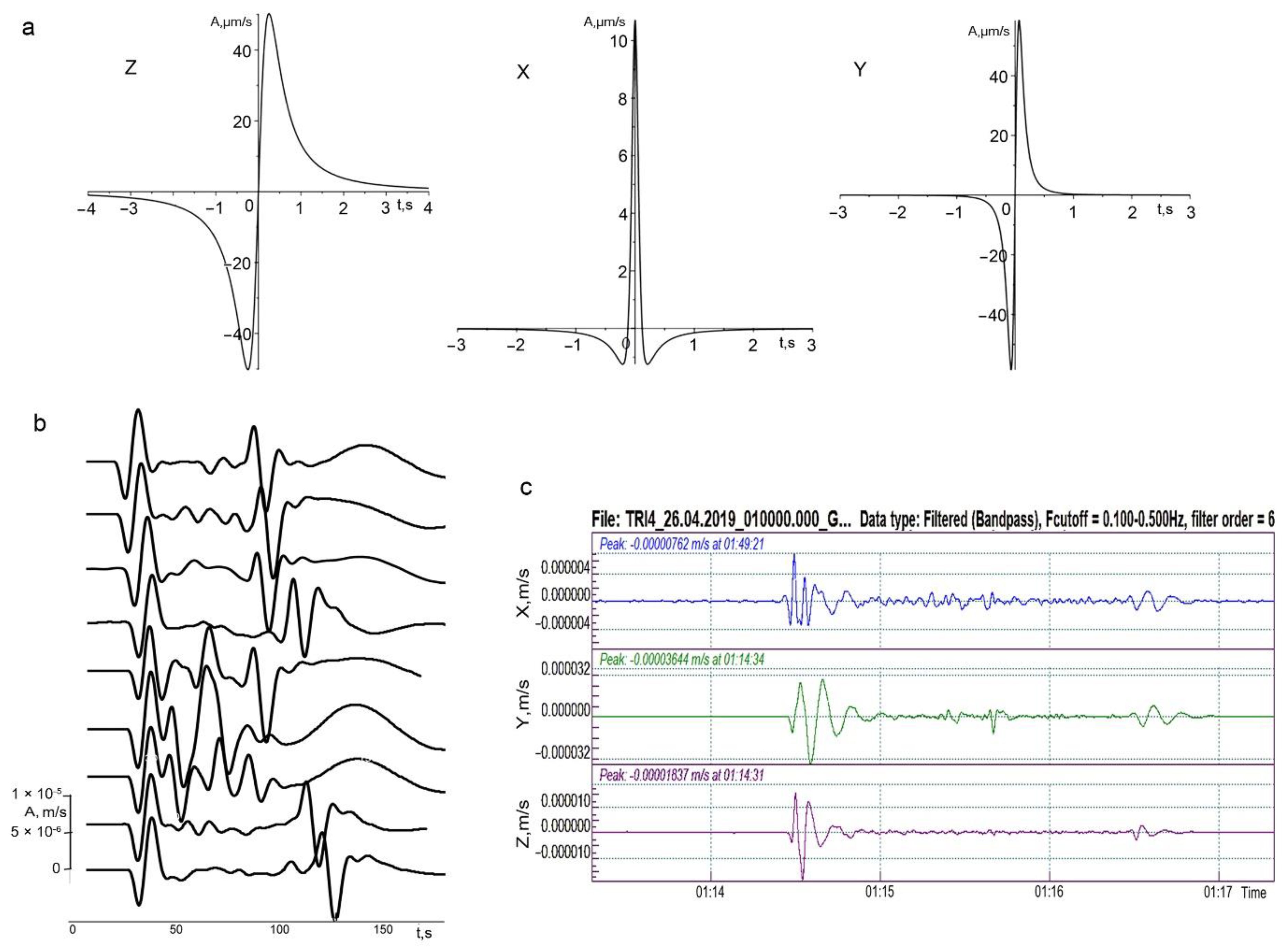
The vibration velocity amplitude of the first arrivals on component $Z$ (A_Z) is inversely proportional to the shear modulus (1) and for real seismograms A_Z is quite simple to measure, so this parameter was adopted to monitor the soil state. In [25], we did not consider the results for horizontal components. Figure 4 shows the calculated waveforms for all vibration velocity components.

For the vertical component, the experimental and calculated waveforms were similar, and the amplitude values corresponded to the observations of 2017 in dry August A_Z ~ 10–70 μm/s (Figure 4b). In 2019, the median value was <A_Z> = 7.5 μm/s and according to (1), indicates a higher value of the μ. This result is realistic, given the difference between heated and frozen soil [47]. For horizontal components, the oscillations were a higher frequency compared to $Z$, based on the waveform visual assessment. Comparison with experimental waveforms, obtained by bandpass filter 0.1–0.5 Hz, agreed with the theory on the prevailing frequencies of the component waveforms, but did not have good agreement with the experiment on signal levels, especially for the $Y$-component.

Thus, Boussinesq’s model describes well the observed experimental features of the first arrival waveforms of the $Z$-components, but does not give an explanation for the lower-frequency horizontal oscillations.

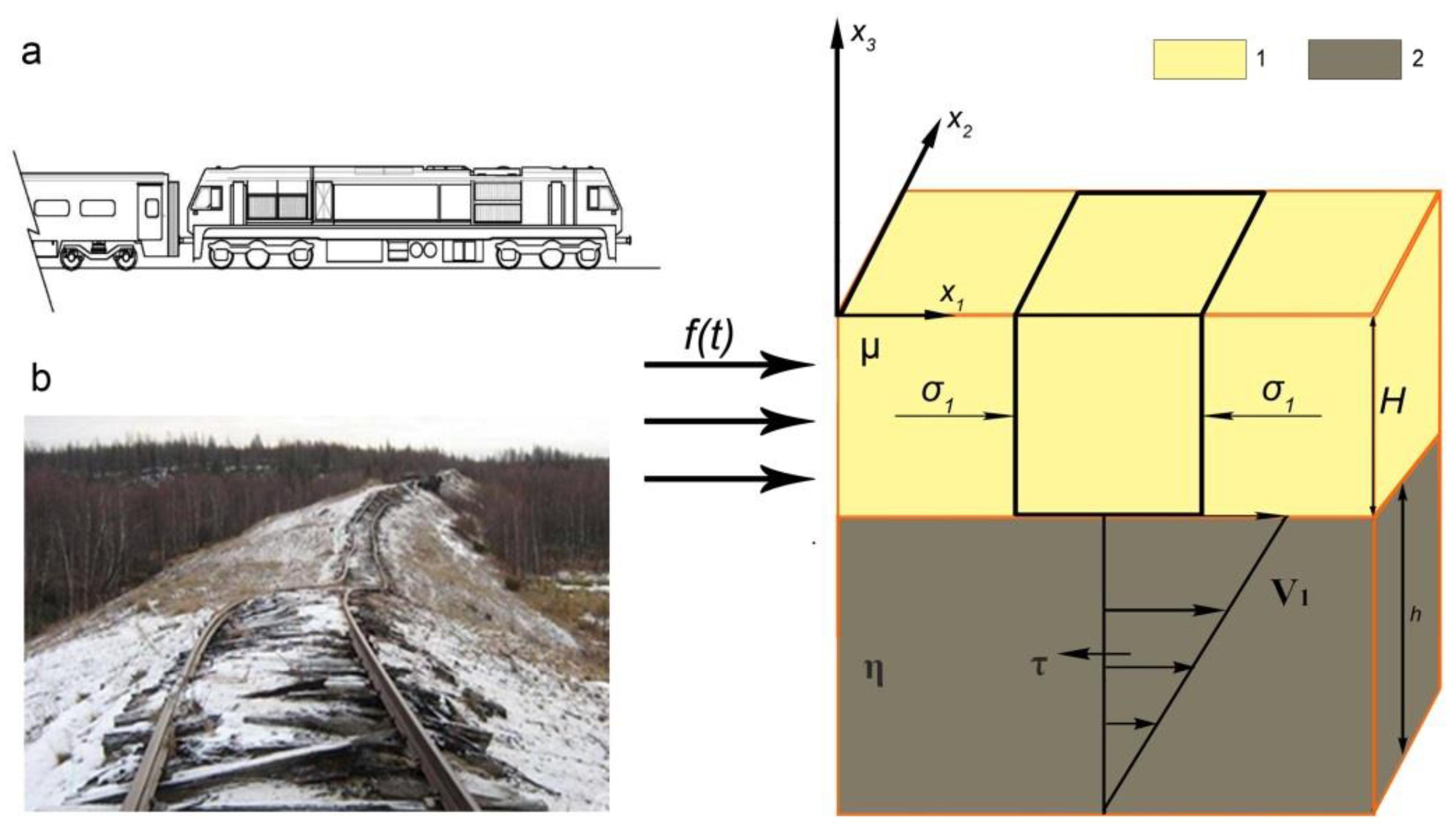
Model 2. Elsasser’s model examines the elastic layer over a viscous half-space and describes the space–temporal distribution of medium stress [48]. In this work, the model is proposed to describe the propagation of stress according to diffusion laws in a horizontal direction from the mid-ocean ridge; the lithosphere consists of an elastic crust and viscous asthenosphere. The model made it possible to explain the delay in platform seismicity relative to the push created by the ridge as well as to estimate the viscosity of the lithosphere. We used the solution obtained in [48], but at a different scale level where the initiating push is created by the train, so the viscous medium can correspond to the low velocity zone, and the upper elastic layer is the overlying soil (Figure 5a). Confirmation of the reality of the model in our case showed typical pictures of path deformation (Figure 5b).

In [48], the response to the push was estimated by the change in time of seismicity, so we used the change in time of the amplitude of oscillations at the observation point as a parameter indicating the “arrival” of the impact. This is possible because the amplitude of the vibration velocity is proportional to the additional deformation [41] and thus, for an elastic medium, to the additional stress.

In the model, we used the following parameter values: H = 2.5 m, h = 4.5 m in accordance with the scheme of the subgrade and the results obtained from the shallow seismic survey [42]. As is well-known, the shear modulus is related to the speed of transverse waves by the following ratio:

$$\mu ={V_s}^2·\rho .$$

(5)

If the density of the gravel-sand mound is 2 g/cm³, $V_s=150$ m/s, then $\mu$ = 0.5 × 10⁸ Pa. We used the well-known formula to calculate the Poisson coefficient:

$$V_P=\sqrt{\frac{2\mu \left(1-\nu \right)}{\rho \left(1-2\nu \right)}},$$

(6)

then $\nu =0.4$ according to the results of shallow seismic prospecting, where the average P-wave velocities vary $V_P=$ 330−440 m/s. The average duration of the train load is T = 80 s.

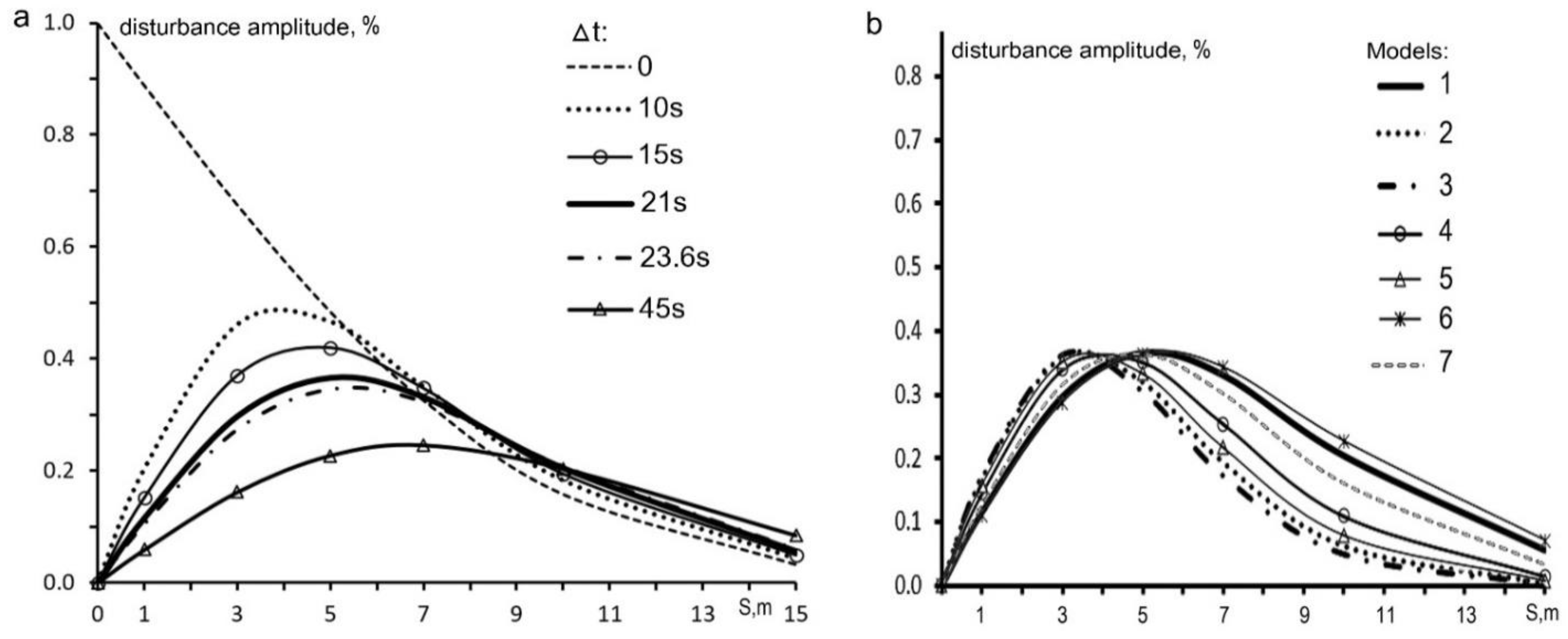
The disturbance amplitude value and the position of its curve maximum depend on the shear modulus of the upper layer and the viscosity of the lower layer. Figure 6 shows the results of calculations of the disturbance amplitudes depending on the distance from the railway, therefore, the movement of the curve maximum with distance from the railway is clearly visible. Different curves correspond to the times when the amplitude reached the maximum after the train passage, in our case, this was parameter $\Delta t$. The disturbance amplitude reached a maximum at about 21 s (Figure 6a) after the train passing at a distance of 5 m (the sensor installation site); the maximum experimental velocity maximum occurred at 23.6 s. The calculation coincided well with the experiment (see Table 1). At the same time, the greater the value of $\Delta t$, the smaller the disturbance amplitude.

Table 2. Different sets of parameters of the railway soil elastic–viscous model.

Models	µ, 108 Pa	η, 109 Pa·s
1	0.4	2
2	0.2	2
3	0.18	2
4	0.2	1.5
5	0.2	1.8
6	0.4	1.8
7	0.3	1.8

contains the values of the soil parameters that we set for modeling, and Figure 6b shows the results. Thus, when the properties of the soils (shear modulus or viscosity coefficient) change, changes in the maximum values of disturbance amplitudes are observed.

4. Discussion

The results of the analytical modeling allowed us to correlate $\Delta t$ and amplitude variations with changes in the shear modulus and/or viscosity coefficient. At this investigation stage, we showed that soil state parameters are not directly measured but can be defined using soil deformation models and measured $\Delta t$ and amplitude values. Of course, we will obtain widespread values of observed parameters for different soil types, which is a separate scientific task and was not considered in this paper.

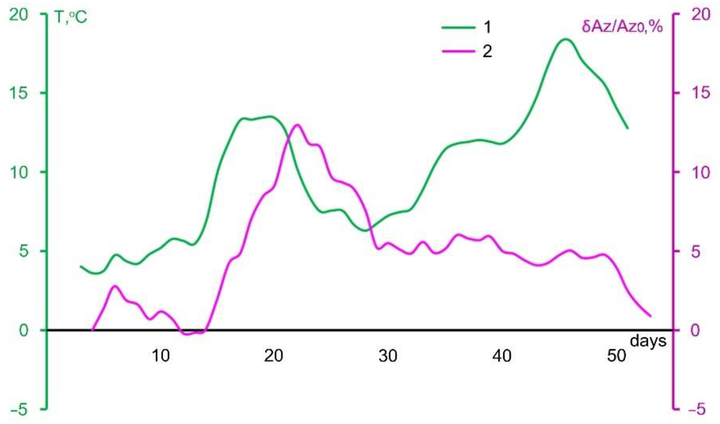
Let us consider the possibility of seasonal changes in the soil state recognition based on the analysis of the seismic records with long-term observations at one site from 23 April to 15 June 2019. Essentially, the ability to detect seasonal changes that are not dangerous processes determines the sensitivity of the selected parameters and the monitoring methodology as a whole.

Figure 7 shows a comparison of the temporal variations for two values: average daily value air temperature and fluctuations from the initial value A_Z0 of the vibration velocity amplitude (in %) on the Z-component (δA/A_Z0). To obtain a comprehensive estimate of the A_Z parameter, we averaged for the day the A_Z values for about 20–30 trains and then for the resulting array, we smoothed with a moving average of seven points (weekly move). Thus, we reduced the dispersion of the A_Z estimate (relative to one obtained by the statistical processing of the data array) by about 10 times (i.e., the accuracy of determining this parameter became, based on Table 1, less than 2%). Note that such accuracy was achieved due to the averaging of parameters for many trains. This result indicates the possibility of replacement when monitoring a signal with good repeatability with statistical processing of a large data array for signals with worse repeatability.

We understand that the observation period was not long enough to make firm conclusions, but we will present a hypothesis for the interpretation of the results shown in Figure 7.

Curve analysis in Figure 7 shows that at low air temperatures at the beginning of the observations (with the ground still frozen), A_Z fluctuations changed little (i.e., the soil was still stiffer than in subsequent days). Seasonal soil freezing is estimated from existing regulatory standards for various regions of Russia. With a sharp rise in temperature, we also observed a rise in δA_Z/A_Z0 to the maximum, where thawing and moisture saturation began, which reduced the shear modulus, which is generally consistent with the data presented in [47]. We noted a characteristic delay in the process by ~5 days relative to the temperature variation. Then, the process in this soil layer ended, even with an increase in temperature, and then, most likely, thawing of the lower layers of the roadbed section occurs. According to the model, we obtained variations in the properties in the upper soil layer to depths of ~1 m, determined by the sensor location.

The largest changes of A_Z in 2019 were about 15%, which, according to Equation (1), occurs when the shear modulus changes by about 15%, or the transverse wave velocity according to (5) by about 7%, which is quite difficult to detect with shallow seismicity.

Thus, through theoretical calculations and field observations, we showed the efficiency of using the first arrival amplitude on the $Z$-component velocity records for soil state monitoring of the railway subgrade. The selected A_Z parameter is quite simply determined during automated processing and is one of the parameters set for subgrade state remote monitoring via cloud platforms.

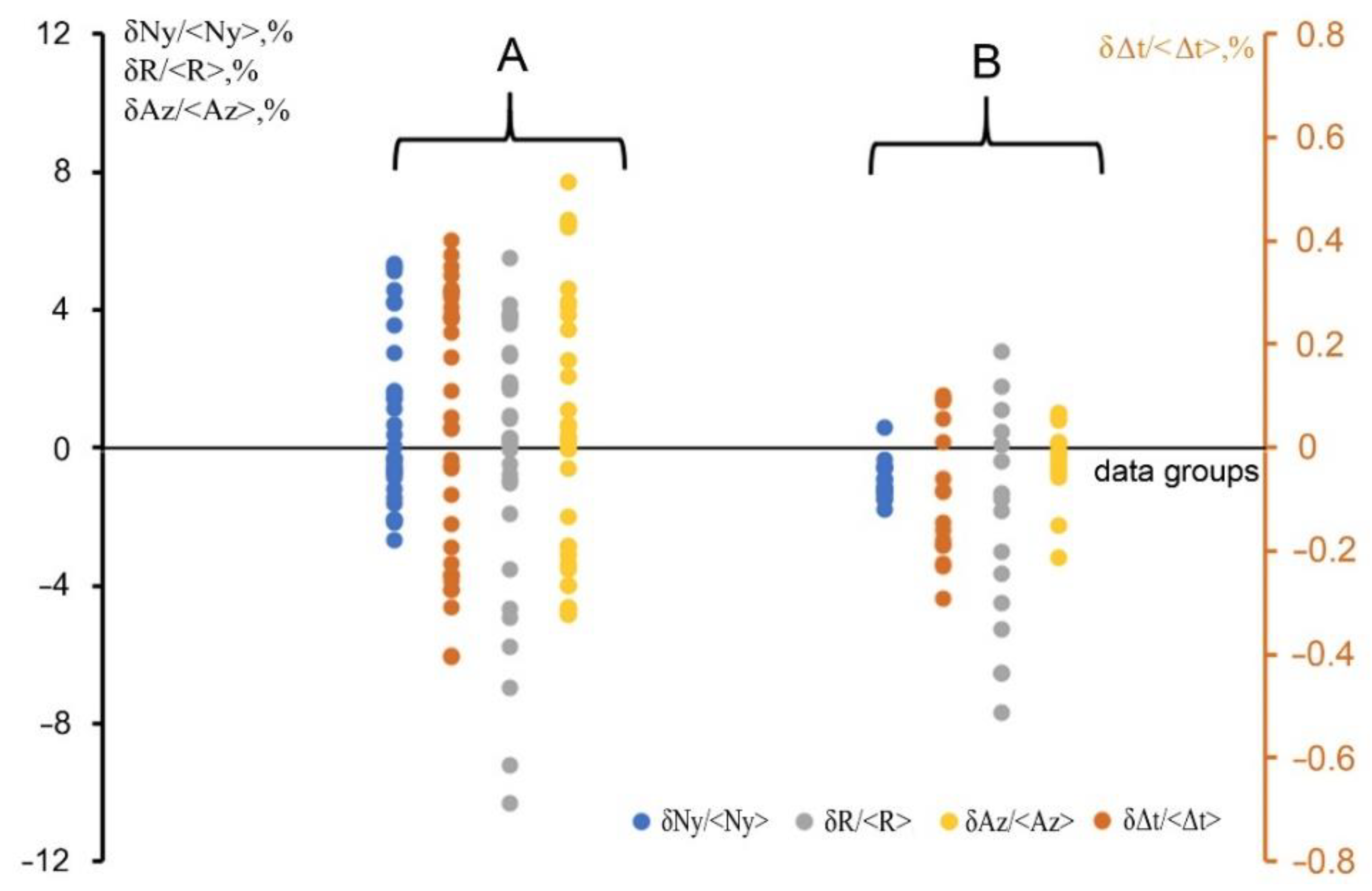
Let us consider parameters R and $\Delta t$. They depend not only on the shear modulus, but also on the underlying medium viscosity [47]. These parameters change in opposite directions during thawing, so it is difficult to make a direct comparison of their time variation and temperature. In accordance with the temperature increase and the A_Z curve in Figure 7, let us assume that after 30 days of observations, thawing in the upper layer is over. For the experimentally obtained arrays, A_Z, R, $\Delta t$ in the low-frequency band and the earlier estimation of the oscillation power ratio in the frequency band 5–8 Hz such as

$$N_Y=(\frac{1}{K}){\sum }_i^K{A}_{Y,i}^2/A_{Z,i}^2$$

fluctuations from the mean value for the entire monitoring interval were calculated using daily averaging and weekly smoothing ($\delta N_y /<N_y>, \delta R/\langle R\rangle , \delta A_Z/\langle A_Z\rangle , \mathsf{\delta }\Delta t/\langle \Delta t\rangle$ in percent) [46]. The resulting fluctuation arrays were divided into two groups—before and after 30 days (Figure 8). Comparison of the variation of parameters for these groups shows that for $\delta N_y /<N_y>, \delta A_Z/\langle A_Z\rangle , \mathsf{\delta }\Delta t/\langle \Delta t\rangle$, the scatter after thawing was much smaller than before it (i.e., when active changes occurred in the medium (thawing, watering, etc.)). Thus, these parameters are suitable for soil condition monitoring. Fluctuations $\delta R/\langle R\rangle$ for the two groups were comparable, however, to understand its sensitivity and suitability for automated monitoring, longer observations are required.

5. Conclusions

The increase in axle loads and the heavy train lengths intensifies the dynamic response of subgrade bed layers, thus bringing new challenges to the serviceability of existing railways. Similar situations were observed in other countries besides Russia. For example, in Canada, the axle loads and traffic volume are continuing to increase. The Canadian National Railway plans to increase the allowable carloads to 130 tons, lengthen trains up to 90 cars, and run up to ten trains per day. However, there still remains the problem of subgrade degradation, location on soft soils, and timely finding of these places. Evaluations made for China showed that the upper limit of a train axle load was approximately 27 t for the currently existing railway lines. Increasing the axle load requires optimizing the design of the subgrade considering its dynamic performances.

Heavy vehicles, based on the example of railway trains, are sources of mechanical vibrations in a wide frequency band range up to long-periods of about 100 s. These oscillations are currently available for seismic observations at distance points of several meters from the track, in our case, we used the broadband sensitive seismometers TC-120s (Nanometrics, Ottawa, Canada). The observed records are suitable for the reliable selection of a useful signal and automated processing of its parameters.

In the band from units of Hz and below, oscillations are the response to the soil deforming impact of vehicles. The vibration parameters in different frequency bands correspond to deformation: in the upper elastic layer up to a depth of about 1 m (highpass filter from 0.1 Hz and higher), and in the deeper parts of the section, as represented by the elastic layer in the elastic-viscous half-space (lowpass filter 0.1 Hz).

When processing seismic records from vehicles, a set of parameters characterizing the soil state of the path is proposed. These are the amplitudes of the extremes in the first arrivals and the amplitudes on characteristic times after the train passage. These parameters depend little on the train characteristics but are determined by the soil deformation properties. We selected an appropriate analytical model that, in our opinion, best describes the dynamic subgrade behavior in the low-frequency range when exposed to a passing train and the simulation results coincided with the experimental results.

The first results of the experimental monitoring of the railway subgrade state in the low-frequency range allow us to assume that the proposed parameters are sensitive to seasonal changes in soils, particularly to the processes of thawing. These changes are an assessment of the sensitivity of the monitoring methodology, which gives hope for the possibility of identifying hazardous processes in the soils at an early stage.

The main limitations of the study at this stage are that we observed changes in the subgrade state in a relatively short time period and did not consider various types of seasonal changes. We did not analyze the reaction of the subgrade located on different soils. The next limitation is that we did not investigate the placement step of seismometers along the railway track. These questions are left for future research.

Currently, we have installed identical seismic monitoring systems on two sections of the Northern Railway in the Arkhangelsk region for a long period (minimum one year). We coordinated these railway sections with our colleagues from the Russian University of Transport (MIIT). One railway site is stable, and the second one is unstable, with a length around 90 m, and there is peat at the base. The distance between them is 120 m. Long-term observations will allow us to record the processes of seasonal freezing and thawing of the subgrade. We will be able to obtain variations in the parameters we found and compare them for two sections. This will allow us to obtain limit values, the extremes of which will indicate the development of negative processes. To evaluate the placement step of seismometers in an unstable area, we will conduct an experiment in which we will change the distance between the sensors and compare the values of various parameters, characterizing the subgrade reaction to the vibration effects created by trains in the ultra-low-frequency range.

Additionally, we will try to use cheaper broadband seismometers but with less stable characteristics. This is because it is necessary to observe different vehicle types (such as planes, heavy cars, etc.). Now we are only at the beginning of research into this technology, so it is difficult to conduct an economic analysis, but such technology is much cheaper than troubleshooting.