Voltage Stabilisation of a Drive System Including a Power Transformer and Asynchronous and Synchronous Motors of Susceptible Motion Transmission

Abstract

A mathematical model is developed of the master circuit of an electric driver system including a power transformer and susceptible motion transmission of asynchronous and synchronous drives. Electric motors drive water pumps by means of motion transmission that comprises two elastic couplings of lumped mechanical parameters and a long shaft of distributed mechanical parameters. Differential equations for oscillatory processes for the long shaft and the elastic couplings are different. The shaft is described with partial derivative Euler–Poisson equations, which, combined with the boundary conditions, form mixed problems from the mathematical point of view. The elastic couplings, on the other hand, are described with the ordinary second type Lagrange equations. Based on the theory of electromagnetic field, the partial differential equations describe the skin effects across the rotor age bars. Vertical pumps are presented by means of a loading torque waveform as a function of the input shaft’s angular velocity. The complex mathematical model serves to analyse electromechanical transient processes across the integrated drive system. Starting from there, conditions of stabilisation of the drive system voltage are determined. Electromechanical state equations are presented in the normal Cauchy form and integrated using the fourth-order Runge–Kutta method. Results of computer simulations are shown with graphics, which are interpreted and described.

1. Introduction

The process of water supply plays an important part in contemporary society. There is a global trend towards high-quality centralised water supply for increasing numbers of consumers. High-power pumping systems operate in the metallurgic, steelmaking, chemical, and electric power industries, for instance. Virtually every large plant has dedicated water and sewage divisions tasked with providing water for production processes [1,2,3,4,5]. Asynchronous drives are normally used to power-pumping systems that use susceptible motion transmissions to drive pump rotors. Asynchronous motors have a range of advantages over other electric motors, although they suffer from the fundamental drawback of consuming high magnetising currents that can reach values of several times the rated currents in transient processes [6,7,8]. Motors in pumping systems are supplied from power transformer secondary windings. The way the power supply grid will respond to drive system processes and quality of electricity needs to be analysed and described, in particular, to what value supply voltage of pump drives will reduce, especially in transient states [9,10,11].

A variety of methods are employed to stabilise voltage. One consists in reducing the power transformer turns ratio, which will in turn increase the supply voltage of motors by way of raising voltage across a power transformer’s secondary winding. In other words, depending on a dynamic state of a drive system, voltage supplied to motors can be adjusted by modifying the turn’s ratio. This approach can be applied to rigid grids. Where grids are not rigid, particularly given many medium and high-power drives, currents across power transformers will grow a lot and, consequently, a plant’s electric power grid will sustain a greater loading.

Another approach is based on a completely different idea—not of changing energetic properties of a system but introducing additional stabilising elements directly to the power supply of a drive system. From the perspective of applied physics, currents flow across these extra elements which, in the steady state, are in counterphase to currents of the power supply system. According to the first Kirchhoff law, total current across an electric unit will fall while voltage will rise. This is the so-called passive power compensation in a drive system in the steady state. Static capacitor batteries are commonly used as compensation devices. The method gets more complicated in the case of high-power drive systems supplied from medium-voltage grids, which requires application of rather costly compensation equipment [12,13,14,15].

There is also a third approach to stabilising voltage in a drive system, which is essentially different to the two described above. If practicable, part of asynchronous drive motors should be replaced with synchronous motors as early as the stage of a drive system design [9,16,17,18,19,20]. In static states, the angle between the vector of a drive system supply voltage and the vector of synchronous machine phase current can be controlled with the well-known V-characteristics (Mordey curves). In transient states, varying excitation currents of synchronous machines lead to regulation effects and consequently to stabilisation of a drive system voltage.

Each of these three methods has its advantages and disadvantages. It is not our intention to analyse them in detail here. A final decision to select a method of, and a solution to, voltage stabilisation of a drive system should evidently address both economic and energetic analyses. We are presenting an energetic analysis of a drive system’s voltage stabilisation by replacing some asynchronous motors with their equivalent synchronous motors. The fact that a variety of oscillation processes arise in electric drives including susceptible motion transmission which impair operations of drive systems in resonant and near-resonant (vibration rumble) states is an important argument in the general analysis [21,22,23,24,25].

The aim of this work is mathematical modelling of transient processes in an electric load assembly. The elements of the assembly are a power transformer and asynchronous and synchronous pump drives with flexible transmission of motion with distributed parameters. Additional goals are:

• Analysis of the power system depending on the value of the excitation current of synchronous motors, taking into account the oscillating mechanical processes in the transmission of motion;
• Simulation test of load assembly states depending on electrical and mechanical parameters.

We analyse pump systems of susceptible motion transmission and lumped and distributed mechanical parameters in drive systems. Thus, the purpose of this study is to analyse transient processes in a drive system including a power transformer, asynchronous and synchronous pump systems of susceptible motion transmission, and long torsional elements of lumped and distributed mechanical parameters.

In order to achieve the above-mentioned goal, mathematical models of all components of the electric load assembly were developed. The main approach of formulating the model is to use the concept of electromechanical energy conversion: electrical components of devices are described by electromagnetic equations taking into account the phenomenon of current displacement in deep-bar cage induction motors. The mechanical components of the electromechanical system are described by the theory of analytical mechanics as components with distributed parameters. On this basis, one comprehensive model of the electric load assembly was developed, with the help of which simulation tests were carried out.

The paper presents the results of the computer simulation, which are analysed and interpreted. The accuracy of the above-mentioned results was verified on the basis of a comparison with the real waveforms occurring in the components of the electric load assembly and included in our articles [11,23,24,26,27].

2. Mathematical Model of an Electromechanical System

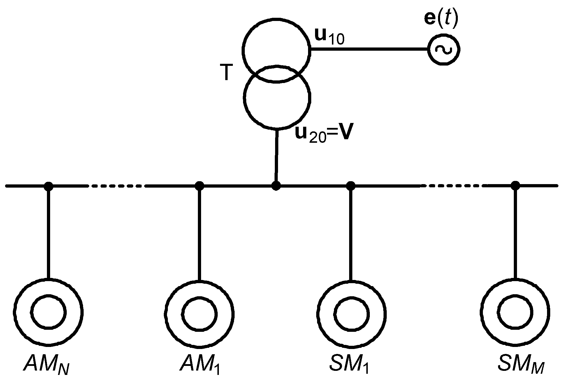
The symbols in Figure 1 stand for: e(t)—columnar vector of phase electromotive forces of a rigid electric power grid, T—power transformer, u₁₀—columnar vector of phase voltages supplied to the power transformer’s primary winding, u₂₀—columnar vector of phase voltages supplied to the power transformer’s secondary winding, V = u₂₀—columnar vector of phase drive system voltages, AM—asynchronous drives, SM—synchronous drives, N—number of asynchronous drives in the drive system, and M—number of synchronous drives in the drive system.

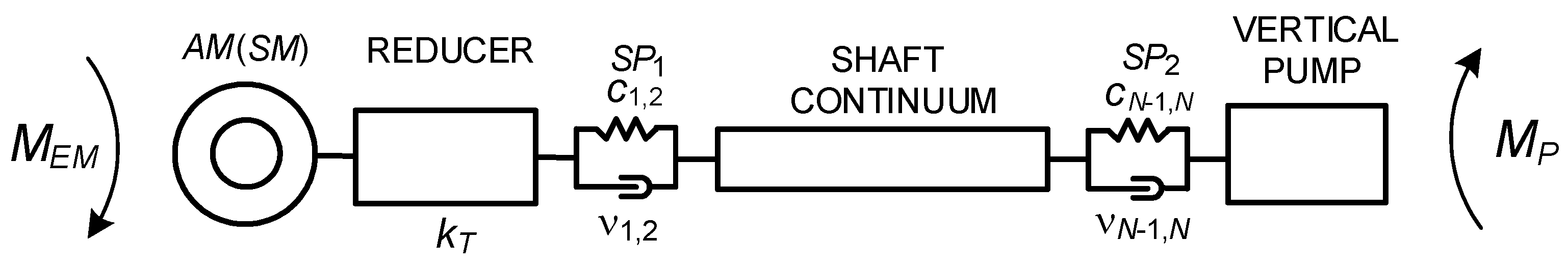
Motion transmission of pumping systems of both the drive types is depicted in Figure 2.

Figure 2 contains the following nomenclature: M_EM—electromagnetic torque of the drive motor, M_P—pump’s hydraulic torque, SP₁—flexible coupling between the rotor and motion transmission long shaft (the first coupling), SP₂—flexible coupling between the motion transmission long shaft and the vertical pump’s input rotor (the second coupling), C_1,2, ν_1,2—rigidity and leakage coefficients of the first coupling, C_N−1,N, ν_N−1,N—rigidity and leakage coefficients of the second coupling, k_T—value of the reducer’s gear.

Mathematical models of the drive system elements will be presented on the basis of Figure 1 and Figure 2 and of [9,10,21,28,29,30,31,32]. A general interdisciplinary theory modifies the Hamilton–Ostrogradsky principle by expanding the Lagrangian with two components: energy of internal and external dissipation and energy of external non-potential forces is applied to mathematical modelling of the drive system’s electric elements. The method is described in [9]. As distinct from the well-known methods, discussed, e.g., in [22,23,29], it enables analysis of both lumped and distributed parameter systems addressing non-linear dependencies between the vectoral functions of the scalar argument. Thus, drive system elements are modelled using the modified interdisciplinary Hamilton–Ostrogradsky principle.

Use of the first Kirchhoff law allows to ignore three-phase equation elements in the model. We assume, therefore, the electromechanical system in Figure 1 works in a symmetrical state and uncompensated associated fluxes in the non-magnetic zone of the power transformer can be ignored [9,11].

When the power transformer is described with equations, parameters of the primary transformer winding are reduced to those of the secondary winding including the transformer voltage ratio [11].

$$\frac{d{i}_{10}}{dt}=A_{11,0}(u_{10}-r_{10}{i}_{10})+A_{12,0}(V-r_{20}{i}_{20})$$

(1)

$$\frac{d{i}_{20}}{dt}=A_{21,0}(u_{10}-r_{10}{i}_{10})+A_{22,0}(V-r_{20}{i}_{20}),\hspace{0.17em}\hspace{0.17em}\hspace{0.17em}\hspace{0.17em}\hspace{0.17em}\hspace{0.17em}\hspace{0.17em}\hspace{0.17em}V\equiv u_{20}$$

(2)

$$A_{11}={\alpha }_{\mathsf{\sigma }1}(1-{\alpha }_{\mathsf{\sigma }1}G)\hspace{0.17em},\hspace{0.17em}\hspace{0.17em}\hspace{0.17em}{A}_{12}=A_{21}=-{\alpha }_{\mathsf{\sigma }1}{\alpha }_{\mathsf{\sigma }2}G\hspace{0.17em},\hspace{0.17em}\hspace{0.17em}\hspace{0.17em}\hspace{0.17em}{A}_{22}={\alpha }_{\mathsf{\sigma }2}(1-{\alpha }_{\mathsf{\sigma }2}G)$$

(3)

$$G\equiv \boxed{\begin{array}{cc}{({\mathsf{\alpha }}_{\mathsf{\sigma }1A}+{\mathsf{\alpha }}_{\mathsf{\sigma }2A}+{\mathsf{\rho }}_A)}^{-1}& \\ & {({\mathsf{\alpha }}_{\mathsf{\sigma }1B}+{\mathsf{\alpha }}_{\mathsf{\sigma }2B}+{\mathsf{\rho }}_B)}^{-1}\end{array}}$$

(4)

$$i_{mA}+i_{mB}+i_{mC}=0\hspace{0.17em},\hspace{0.17em}\hspace{0.17em}\hspace{0.17em}\hspace{0.17em}\hspace{0.17em}{\mathsf{\psi }}_{mA}+{\mathsf{\psi }}_{mB}+{\mathsf{\psi }}_{mC}=0$$

(5)

$$i_m\equiv {\boxed{\begin{array}{cc}{i}_{mA}& i_{mB}\end{array}}}^{\mathrm{T}}={\boxed{\begin{array}{cc}{i}_{1A}+i_{2A}& i_{1B}+i_{2B}\end{array}}}^{\mathrm{T}}$$

(6)

$$\tau \equiv \boxed{\begin{array}{cc}{\mathsf{\tau }}_A& \\ & {\mathsf{\tau }}_B\end{array}}\hspace{0.17em}=\mathrm{diag}({\mathsf{\tau }}_A;\hspace{0.17em}{\mathsf{\tau }}_B)\hspace{0.17em},\hspace{0.17em}\hspace{0.17em}\hspace{0.17em}\hspace{0.17em}{\mathsf{\tau }}_j={\left(\frac{{\mathsf{\psi }}_{m,j}}{i_{m,j}}\right)}^{-1}$$

(7)

$$\rho \equiv {\tau }^{\partial }\equiv \boxed{\begin{array}{cc}{\mathsf{\rho }}_A& \\ & {\mathsf{\rho }}_B\end{array}}\hspace{0.17em}=\mathrm{diag}({\mathsf{\rho }}_A\hspace{0.17em};\hspace{0.17em}{\mathsf{\rho }}_B)\hspace{0.17em},\hspace{0.17em}\hspace{0.17em}\hspace{0.17em}\hspace{0.17em}{\mathsf{\rho }}_j\equiv {\mathsf{\tau }}_j^{\partial }={\left(\frac{\partial {\mathsf{\psi }}_{m,j}}{\partial i_{m,j}}\right)}^{-1},\hspace{0.17em}\hspace{0.17em}\hspace{0.17em}j=A\hspace{0.17em},\hspace{0.17em}B$$

(8)

where i₁₀, i₂₀—columnar vectors of phase currents of the transformer’s primary and secondary windings, respectively, r₀—matrix of winding resistances, α_σ1, α_σ2—matrices of reverse transformer leakage inductances, A₀—matrix of reverse transformer inductances, i_m—columnar vector of transformer magnetising currents, ψ_m,j—working associated transformer fluxes, to be determined by means of the power transformer magnetising curve, τ—matrix of reverse magnetising inductances, ρ—matrix of reverse differential magnetising inductances, and j = A,B—indices of three-phase system phases.

When modelling the asynchronous motor, parameters of rotor winding (virtual equivalent three-phase system) are reduced to the stator winding parameters considering the current and voltage gear k_i, k_u. Deep bar cage asynchronous motors are adopted for the purposes of analysis, where current displacement across the rotor cage bars is addressed [9,30] based on the electromagnetic field theory, which helps to calculate the voltage across the rotor cage bars with ordinary and partial differential equations:

$$\frac{d{i}_{S,k}}{dt}=A_{S,k}(V-r_{S,k}{i}_{S,k})+A_{SR,k}(-u_{R,k}-{\Omega }_k{\Psi }_{R,k}-r_{RL,k}{i}_{R,k})$$

(9)

$$\frac{d{i}_{R,k}}{dt}=A_{RS,k}(V-r_{S,k}{i}_{S,k})+A_{R,k}(-u_{R,k}-{\Omega }_k{\Psi }_{R,k}-r_{RL,k}{i}_{R,k})+{\Omega }_k{i}_{R,k},\hspace{0.17em}\hspace{0.17em}\hspace{0.17em}\hspace{0.17em}\hspace{0.17em}V\equiv u_{20}$$

(10)

$$A_S={\alpha }_{\mathsf{\sigma }S}(1-{\alpha }_{\mathsf{\sigma }S}G)\hspace{0.17em},\hspace{0.17em}\hspace{0.17em}\hspace{0.17em}\hspace{0.17em}\hspace{0.17em}\hspace{0.17em}{A}_{SR}=-{\alpha }_{\mathsf{\sigma }S}{\alpha }_{\mathsf{\sigma }RL}G{\Pi }_1\hspace{0.17em},\hspace{0.17em}\hspace{0.17em}\hspace{0.17em}\hspace{0.17em}\hspace{0.17em}\hspace{0.17em}{A}_{RS}=-{\Pi }_1^{-1}{\alpha }_{\mathsf{\sigma }S}{\alpha }_{\mathsf{\sigma }RL}G\hspace{0.17em},\hspace{0.17em}\hspace{0.17em}\hspace{0.17em}\hspace{0.17em}\hspace{0.17em}\hspace{0.17em}\hspace{0.17em}{A}_R={\Pi }_1^{-1}{\alpha }_{\mathsf{\sigma }RL}(1-{\alpha }_{\mathsf{\sigma }RL}G){\Pi }_1$$

(11)

$$G_S={\alpha }_{\mathsf{\sigma }S}G\hspace{0.17em},\hspace{0.17em}\hspace{0.17em}\hspace{0.17em}\hspace{0.17em}\hspace{0.17em}{G}_R={\alpha }_{\mathsf{\sigma }RL}G\hspace{0.17em},\hspace{0.17em}\hspace{0.17em}\hspace{0.17em}\hspace{0.17em}\hspace{0.17em}\hspace{0.17em}G=\boxed{\begin{array}{cc}B+b_A{i}_A& b_B{i}_A\\ b_A{i}_B& B+b_B{i}_B\end{array}}$$

(12)

$${\Pi }_1=\frac{2}{\sqrt{3}}\boxed{\begin{array}{cc}\sin (k_T{p}_0\mathsf{\gamma }+120°)& -\sin (k_T{p}_0\mathsf{\gamma })\\ \sin (k_T{p}_0\mathsf{\gamma })& -\sin (k_T{p}_0\mathsf{\gamma }-120°)\end{array}}\hspace{0.17em},\hspace{0.17em}\hspace{0.17em}\hspace{0.17em}\hspace{0.17em}{\Pi }_1^{-1}=\frac{2}{\sqrt{3}}\boxed{\begin{array}{cc}-\sin (k_T{p}_0\mathsf{\gamma }-120°)& \sin (k_T{p}_0\mathsf{\gamma })\\ -\sin (k_T{p}_0\mathsf{\gamma })& \sin (k_T{p}_0\mathsf{\gamma }+120°)\end{array}}$$

(13)

$$B=1/({\mathsf{\alpha }}_{\mathsf{\sigma }S}+{\mathsf{\alpha }}_{\mathsf{\sigma }RL}+\mathsf{\tau })\hspace{0.17em},\hspace{0.17em}\hspace{0.17em}\hspace{0.17em}R=1/({\mathsf{\alpha }}_{\mathsf{\sigma }S}+{\mathsf{\alpha }}_{\mathsf{\sigma }RL}+\mathsf{\rho })\hspace{0.17em},\hspace{0.17em}\hspace{0.17em}\hspace{0.17em}\hspace{0.17em}b=\frac{2}{3}\frac{R-B}{i_m^2}\hspace{0.17em},\hspace{0.17em}\hspace{0.17em}\hspace{0.17em}\hspace{0.17em}{b}_A=b(2i_A+i_B)\hspace{0.17em},\hspace{0.17em}\hspace{0.17em}\hspace{0.17em}\hspace{0.17em}{b}_B=b(2i_B+i_A)$$

(14)

$$i_m=\hspace{0.17em}2\sqrt{(i_A^2+i_A{i}_B+i_B^2)/3}\hspace{0.17em},\hspace{0.17em}\hspace{0.17em}\hspace{0.17em}\hspace{0.17em}\hspace{0.17em}\mathsf{\tau }=\frac{1}{L_m}={\left(\frac{{\mathsf{\psi }}_m}{i_m}\right)}^{-1},\hspace{0.17em}\hspace{0.17em}\hspace{0.17em}\hspace{0.17em}\mathsf{\rho }={\left(\frac{\partial {\mathsf{\psi }}_m}{\partial i_m}\right)}^{-1},\hspace{0.17em}\hspace{0.17em}\hspace{0.17em}\hspace{0.17em}{\Omega }_1=\frac{k_T{p}_0\mathsf{\omega }}{\sqrt{3}}\boxed{\begin{array}{cc}1& 2\\ -1& -2\end{array}}$$

(15)

$$i\equiv {\boxed{\begin{array}{cc}{i}_A& i_B\end{array}}}^{\mathrm{T}}={\boxed{\begin{array}{cc}{i}_{SA}& i_{SB}\end{array}}}^{\mathrm{T}}+{\Pi }_1{\boxed{\begin{array}{cc}{i}_{RA}& i_{RB}\end{array}}}^{\mathrm{T}}={\boxed{\begin{array}{cc}{i}_{SA}& i_{SB}\end{array}}}^{\mathrm{T}}+{\boxed{\begin{array}{cc}{i}_{RA}^{{\mathsf{\Pi }}_1}& i_{RB}^{{\mathsf{\Pi }}_1}\end{array}}}^{\mathrm{T}}\hspace{0.17em}\hspace{0.17em},\hspace{0.17em}\hspace{0.17em}\hspace{0.17em}\hspace{0.17em}{\Psi }_R=\frac{1}{{\mathsf{\alpha }}_{\mathsf{\sigma }RL}}{i}_R+\frac{1}{\mathsf{\tau }}i$$

(16)

where Ψ_R—columnar vector of main associated fluxes of the rotor, Π₁—matrix of angle transformations, Ω₁—matrix of angular rotational speeds of asynchronous motor in angle coordinates, u_R—columnar vector of voltages across the rotor cage bars, p₀—number of machine pole pairs, γ—angle of rotor rotation, ω—angular velocity of the rotor, i_m—spatial vector of motor magnetisation, ψ_m (i_m)—working flux of machine magnetisation, L_m—inductance of machine magnetisation, and k = N—number of asynchronous motors in the drive system.

Voltages across the rotor cage bars will be determined according to the theorem of voltage on the deep bar wire surface [9]:

$$u_R=E(0)l$$

(17)

where E(0)—electric intensity on the deep bar surface, and l—length of a deep bar.

E(0) will be derived from Maxwell’s theory [9]:

$$\frac{\partial H}{\partial t}=-\frac{\mathsf{\nu }}{\mathsf{\gamma }}\nabla \times \nabla \times H\hspace{0.17em},\hspace{0.17em}\hspace{0.17em}\hspace{0.17em}\hspace{0.17em}E=\frac{1}{\mathsf{\gamma }}\nabla \times H\hspace{0.17em},\hspace{0.17em}\hspace{0.17em}\hspace{0.17em}\hspace{0.17em}\mathsf{\nu }=\frac{1}{\mathsf{\mu }}$$

(18)

where H, E—vectors of the magnetic and electric field intensity, respectively, γ—specific electric conductance of a wire in a rotor deep bar; μ—magnetic permeability of conductor material in a rotor deep bar.

In a cylindrical system of coordinates, (18) will be expressed as [9]:

$$\frac{\partial H_j}{\partial t}=\frac{\mathsf{\nu }}{\mathsf{\gamma }}\frac{{\partial }^2{H}_j}{\partial z^2}\hspace{0.17em}\hspace{0.17em},\hspace{0.17em}\hspace{0.17em}\hspace{0.17em}{E}_n=-\frac{k_u{k}_i}{\mathsf{\gamma }}\frac{\partial H_j}{\partial z}\hspace{0.17em},\hspace{0.17em}\hspace{0.17em}\hspace{0.17em}\hspace{0.17em}\hspace{0.17em}\hspace{0.17em}j=A\hspace{0.17em},B$$

(19)

where k_u, k_i—voltage and current reduces coefficients of machine transformation, and z—coordinate oriented into a cylindrical system deep bar.

Boundary conditions for the first expression in Equation (19) will be determined according to the law of current surge [9]:

$${H_j|}_{z=0}=\frac{i_{R,n}}{a}\hspace{0.17em}\hspace{0.17em},\hspace{0.17em}\hspace{0.17em}\hspace{0.17em}\hspace{0.17em}\hspace{0.17em}\hspace{0.17em}\hspace{0.17em}{H_j|}_{z=h}=0\hspace{0.17em},\hspace{0.17em}\hspace{0.17em}\hspace{0.17em}\hspace{0.17em}\hspace{0.17em}\hspace{0.17em}j=A\hspace{0.17em},B$$

(20)

where a—deep bar width, and h—bar depth in relation to the coordinate z.

Discretisation of the first expression in Equation (19) by means of the straight-line method will produce:

$$\frac{d{H}_{j,n}}{dt}=\frac{\mathsf{\nu }}{\mathsf{\gamma }{(\Delta z)}^2}(H_{j,n-1}-2H_{j,n}+H_{j,n+1})\hspace{0.17em},\hspace{0.17em}\hspace{0.17em}\hspace{0.17em}\hspace{0.17em}\hspace{0.17em}\hspace{0.17em}\hspace{0.17em}j=A\hspace{0.17em},B,\hspace{0.17em}\hspace{0.17em}\hspace{0.17em}\hspace{0.17em}\hspace{0.17em}n=2,3,\dots ,T-1$$

(21)

where Δz = h/(T − 1)—discretisation step, and T—number of discretisation nodes relative to the coordinate z. Normally, T ≥ 10.

Approximating the spatial derivative in the second expression of Equation (19) using Lagrange’s formula [9] produces the needed function of voltage across the rotor cage bars, see (17):

$$u_{R,j}=-l\frac{k_u{k}_i}{2\mathsf{\gamma }\Delta z}(-3H_{j,1}+4H_{j,2}-H_{j,3})\hspace{0.17em},\hspace{0.17em}\hspace{0.17em}\hspace{0.17em}\hspace{0.17em}\hspace{0.17em}\hspace{0.17em}\hspace{0.17em}\hspace{0.17em}\hspace{0.17em}\hspace{0.17em}j=A\hspace{0.17em},B$$

(22)

Electromagnetic torque of the asynchronous motor will be determined in the usual way [9]:

$$M_{EM}=\sqrt{3}{k}_T{p}_0(i_{SB}{i}_{RA}^{\Pi }-i_{SA}{i}_{RB}^{\Pi })/\mathsf{\tau }$$

(23)

When modelling the synchronous motor, stator (armature) winding parameters are reduced to those of the rotor winding considering the current and voltage gear k_i, k_u. Synchronous motors with salient rotor poles are analysed. We note the synchronous motor model is different to that of the asynchronous motor. There are three currents in the synchronous motor: two in the longitudinal axis d-d and one in the transverse axis q-q, while the phase C current across the stator is excluded. Then, in order to meet the law of matrix multiplication, a topological matrix B is introduced:

$$\frac{d{i}_{S,m}}{dt}=A_{S,m}(V-r_{S,m}{i}_{S,m}-{\Omega }_m{\Psi }_{S,m})+A_{SR,m}{B}^{\mathrm{T}}(u_{R,m}-r_{R,m}{i}_{R,m})+{\Omega }_m{i}_{S,m}$$

(24)

$$\frac{d{i}_{R,m}}{dt}=B{A}_{RS,m}(V-r_{S,m}{i}_{S,m}-{\Omega }_m{\Psi }_{S,m})+A_{R,m}(u_{R,m}-r_{R,m}{i}_{R,m})$$

(25)

$$A_S={\Pi }^{-1}{\alpha }_{\mathsf{\sigma }S}(1-{\alpha }_{\mathsf{\sigma }S}G)\Pi ,\hspace{0.17em}\hspace{0.17em}\hspace{0.17em}\hspace{0.17em}{A}_{SR}=-{\alpha }_{\mathsf{\sigma }S}{B}^{\mathrm{T}}{\alpha }_{\mathsf{\sigma }R}BG\Pi ,\hspace{0.17em}\hspace{0.17em}\hspace{0.17em}\hspace{0.17em}{A}_{RS}=-{\Pi }^{-1}{\alpha }_{\mathsf{\sigma }S}{B}^{\mathrm{T}}{\alpha }_{\mathsf{\sigma }R}BG,\hspace{0.17em}\hspace{0.17em}\hspace{0.17em}\hspace{0.17em}{A}_R={\alpha }_{\mathsf{\sigma }R}(1-{\alpha }_{\mathsf{\sigma }R}BG)$$

(26)

$${\Psi }_S\equiv {({\Psi }_{SA},\hspace{0.17em}{\Psi }_{SB})}^{\mathrm{T}},\hspace{0.17em}\hspace{0.17em}\hspace{0.17em}\hspace{0.17em}\hspace{0.17em}{\Psi }_R\equiv {({\Psi }_D,\hspace{0.17em}{\Psi }_Q,{\Psi }_f)}^{\mathrm{T}},\hspace{0.17em}\hspace{0.17em}\hspace{0.17em}\hspace{0.17em}\hspace{0.17em}\hspace{0.17em}\hspace{0.17em}\hspace{0.17em}{i}_S\equiv {(i_{SA},\hspace{0.17em}{i}_{SB})}^{\mathrm{T}},\hspace{0.17em}\hspace{0.17em}\hspace{0.17em}\hspace{0.17em}\hspace{0.17em}\hspace{0.17em}\hspace{0.17em}\hspace{0.17em}{i}_R\equiv {(i_D,\hspace{0.17em}{i}_Q,i_f)}^{\mathrm{T}}$$

(27)

$$u_S\equiv {(u_{SA},\hspace{0.17em}{u}_{SB})}^{\mathrm{T}},\hspace{0.17em}\hspace{0.17em}\hspace{0.17em}\hspace{0.17em}\hspace{0.17em}{u}_R\equiv {(0,0,\hspace{0.17em}{u}_f)}^{\mathrm{T}},\hspace{0.17em}\hspace{0.17em}\hspace{0.17em}\hspace{0.17em}\hspace{0.17em}{r}_S\equiv \mathrm{diag}(r_S,\hspace{0.17em}\hspace{0.17em}{r}_S),\hspace{0.17em}\hspace{0.17em}\hspace{0.17em}\hspace{0.17em}\hspace{0.17em}\hspace{0.17em}{r}_R\equiv \mathrm{diag}(r_D,\hspace{0.17em}{r}_Q,\hspace{0.17em}{r}_f)$$

(28)

$$L_{\mathsf{\sigma }}{}_S\equiv \mathrm{diag}(L_{\mathsf{\sigma }S},\hspace{0.17em}{L}_{\mathsf{\sigma }S}),\hspace{0.17em}\hspace{0.17em}\hspace{0.17em}\hspace{0.17em}\hspace{0.17em}{L}_{\mathsf{\sigma }}{}_R\equiv \mathrm{diag}(L_{\mathsf{\sigma }D},\hspace{0.17em}{L}_{\mathsf{\sigma }Q},\hspace{0.17em}{L}_{\mathsf{\sigma }f}),\hspace{0.17em}\hspace{0.17em}\hspace{0.17em}\hspace{0.17em}\hspace{0.17em}{L}_m\equiv \mathrm{diag}(L_d,\hspace{0.17em}{L}_q)\hspace{0.17em},\hspace{0.17em}\hspace{0.17em}\hspace{0.17em}\hspace{0.17em}\hspace{0.17em}{B}^{\mathrm{T}}\equiv \left[\begin{array}{ccc}1& 0& 1\\ 0& 1& 0\end{array}\right]$$

(29)

$${\alpha }_m=L_m^{-1}=\mathrm{diag}({\mathsf{\alpha }}_d,\hspace{0.17em}{\mathsf{\alpha }}_q)=\mathrm{diag}\left(\frac{1}{L_d},\hspace{0.17em}\frac{1}{L_q}\right),\hspace{0.17em}\hspace{0.17em}\hspace{0.17em}\hspace{0.17em}\hspace{0.17em}\hspace{0.17em}\hspace{0.17em}\hspace{0.17em}\hspace{0.17em}\hspace{0.17em}G=\boxed{\begin{array}{cc}\frac{1}{{\mathsf{\alpha }}_d+{\mathsf{\alpha }}_{\mathsf{\sigma }S}+{\mathsf{\alpha }}_{\mathsf{\sigma }f}+{\mathsf{\alpha }}_{\mathsf{\sigma }D}}& \\ & \frac{1}{{\mathsf{\alpha }}_q+{\mathsf{\alpha }}_{\mathsf{\sigma }S}+{\mathsf{\alpha }}_{\mathsf{\sigma }Q}}\end{array}},\hspace{0.17em}\hspace{0.17em}\hspace{0.17em}\hspace{0.17em}\hspace{0.17em}\hspace{0.17em}\hspace{0.17em}\hspace{0.17em}\hspace{0.17em}\hspace{0.17em}\hspace{0.17em}\hspace{0.17em}\hspace{0.17em}\Omega =k_T{p}_0\mathsf{\omega }\boxed{\begin{array}{cc}& -1\\ 1& \end{array}}$$

(30)

$$\Pi \equiv \hspace{0.17em}\hspace{0.17em}\hspace{0.17em}\frac{2}{\sqrt{3}}\boxed{\begin{array}{cc}-\sin (k_T{p}_0\mathsf{\gamma }-120°)& \sin (k_T{p}_0\mathsf{\gamma })\\ -\cos (k_T{p}_0\mathsf{\gamma }-120°)& \cos (k_T{p}_0\mathsf{\gamma })\end{array}}\hspace{0.17em},\hspace{0.17em}\hspace{0.17em}\hspace{0.17em}\hspace{0.17em}{\Pi }_{}^{-1}\equiv \hspace{0.17em}\hspace{0.17em}\hspace{0.17em}\boxed{\begin{array}{cc}\cos (k_T{p}_0\mathsf{\gamma })& -\sin (k_T{p}_0\mathsf{\gamma })\\ \cos (k_T{p}_0\mathsf{\gamma }-120°)& -\sin (k_T{p}_0\mathsf{\gamma }-120°)\end{array}}$$

(31)

$${\psi }_S={\Pi }^{-1}{\psi }_m=L_m{i}_m=L_m\left(i_S+{\Pi }^{-1}{B}^{\mathrm{T}}{i}_R\right)$$

(32)

where Ω—matrix of angular rotational speeds of the synchronous machine in rectangular coordinates, Π—Park matrix of rectangular transformations, d—index related to parameters in the machine’s longitudinal axis, q—index related to parameters in the machine’s transverse axis, f—index related to parameters of the excitation winding, D—index related to parameters of the damping winding in the longitudinal axis d, Q—index related to parameters of the damping winding in the transverse axis q, and m = M—number of synchronous drives in the drive system.

Electromagnetic torque of the synchronous motor will be computed in the ordinary manner [9]:

$$M_{EM}=\sqrt{3}{k}_T{p}_0({\mathsf{\psi }}_{SB}{i}_{SA}-{\mathsf{\psi }}_{SA}{i}_{SB})$$

(33)

3. Mathematical Model of a Pumping System’s Motion Transmission

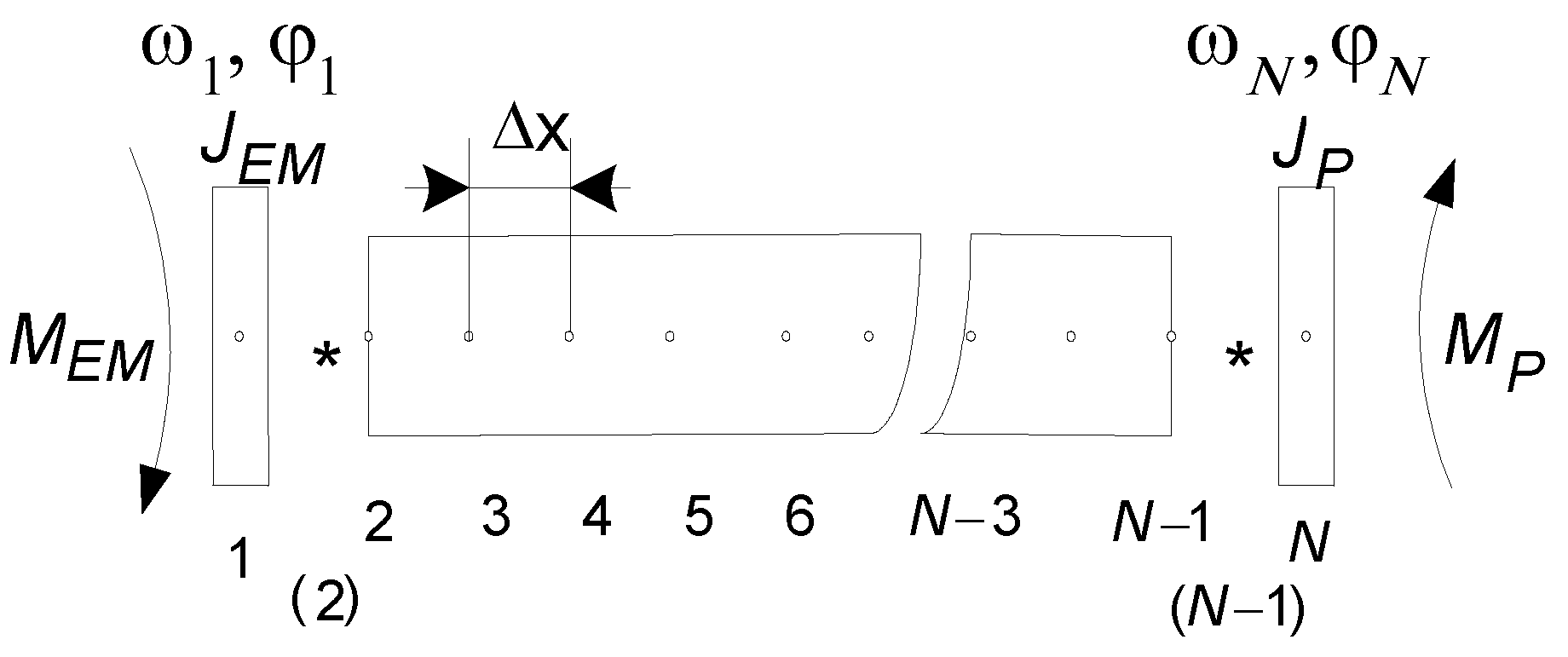
Motion transmissions in asynchronous and synchronous drives are presented as torsional elements of lumped and distributed parameters. We will then also present a mathematical model of an assembly on the basis of the generalised interdisciplinary method [9] that serves to develop the models of a power transformer and drive motors. For an improved visualisation of the modelling process of the mechanical subsystem, a calculation scheme of the motion transmission is shown in Figure 3.

Figure 3 includes the following symbols: J_EM—moment of inertia of the motor’s drive rotor, J_P—moment of inertia of the hydraulic pump rotor recalculated considering the reducer gear, y, ω₁, φ₁—angular velocity and rotation angle of the drive motor rotor, ω_N, φ_N—angular velocity and rotation angle of the vertical pump rotor, Δx—discretisation step of the long shaft equation, *—fictitious discretization node, and N—number of discretisation nodes.

The equation of oscillations of the drive motion transmission long shaft is as follows [24,28]:

$$\frac{d{\mathsf{\omega }}_1}{dt}=\frac{1}{k_T^2{J}_{EM}}\left(c_{1,2}({\mathsf{\phi }}_2-{\mathsf{\phi }}_1)+{\mathsf{\nu }}_{1,2}({\mathsf{\omega }}_2-{\mathsf{\omega }}_1)+k_T{M}_{EM}\right)$$

(34)

$$\frac{d{\mathsf{\omega }}_N}{dt}=-\frac{1}{J_N}(M_P-c_{N-1,N}({\mathsf{\phi }}_N-{\mathsf{\phi }}_{N-1})-{\mathsf{\nu }}_{N-1,N}({\mathsf{\omega }}_N-{\mathsf{\omega }}_{N-1}))$$

(35)

$$\frac{{\partial }^2\mathsf{\phi }(x,t)}{\partial t^2}=\frac{G}{\mathsf{\rho }}\frac{{\partial }^2\mathsf{\phi }(x,t)}{\partial x^2}+\frac{\mathsf{\xi }}{\mathsf{\rho }{J}_p}\frac{{\partial }^2\mathsf{\phi }(x,t)}{\partial x^2}$$

(36)

where G—transverse torsion module, ξ—coefficient of shaft internal leakage; x—current coordinate along the shaft; ρ—density of shaft material; J_p—polar moment of shaft inertia, and φ(x,t)—angle of shaft rotation.

Poincaré boundary conditions of the third type [25] are formulated on the basis of d’Alembert law [9], cf. Figure 2 and Figure 3 will be attached to the shaft Equation (36):

$${G{J}_p\frac{\partial \mathsf{\phi }(x,t)}{\partial x}|}_{x=0}+{\mathsf{\xi }\frac{\partial \mathsf{\omega }(x,t)}{\partial x}|}_{x=0}+c_{1,2}({\mathsf{\phi }}_1-{\mathsf{\phi }}_2)+{\mathsf{\nu }}_{1,2}({\mathsf{\omega }}_1-{\mathsf{\omega }}_2)=0$$

(37)

$${G{J}_p\frac{\partial \mathsf{\phi }(x,t)}{\partial x}|}_{x=l}+{\mathsf{\xi }\frac{\partial \mathsf{\omega }(x,t)}{\partial x}|}_{x=l}-c_{N-1,N}({\mathsf{\phi }}_{N-1}-{\mathsf{\phi }}_N)-{\mathsf{\nu }}_{N-1,N}({\mathsf{\omega }}_{N-1}-{\mathsf{\omega }}_N)=0$$

(38)

Discretisation of (36)–(38) with the straight-line method will produce:

$$\frac{d{\mathsf{\omega }}_2}{dt}=\frac{2\left(c_{1,2}({\mathsf{\phi }}_1-{\mathsf{\phi }}_2)+{\mathsf{\nu }}_{1,2}({\mathsf{\omega }}_1-{\mathsf{\omega }}_2)\right)}{\mathsf{\rho }{J}_p\Delta x}-\frac{2\left(J_{p}G({\mathsf{\phi }}_2-{\mathsf{\phi }}_3)+\mathsf{\xi }({\mathsf{\omega }}_2-{\mathsf{\omega }}_3)\right)}{\mathsf{\rho }{J}_p{(\Delta x)}^2}$$

(39)

$$\frac{d{\mathsf{\omega }}_{N-1}}{dt}=\frac{2\left(J_{p}G({\mathsf{\phi }}_{N-2}-{\mathsf{\phi }}_{N-1})+\mathsf{\xi }({\mathsf{\omega }}_{N-2}-{\mathsf{\omega }}_{N-1})\right)}{\mathsf{\rho }{J}_p{(\Delta x)}^2}-\frac{2\left(c_{N-1,N}({\mathsf{\phi }}_{N-1}-{\mathsf{\phi }}_N)+{\mathsf{\nu }}_{N-1,N}({\mathsf{\omega }}_{N-1}-{\mathsf{\omega }}_N)\right)}{\mathsf{\rho }{J}_p\Delta x}$$

(40)

$$\frac{d{\mathsf{\omega }}_j}{dt}=\frac{\mathsf{\xi }}{\mathsf{\rho }{J}_p{(\Delta x)}^2}\left({\mathsf{\omega }}_{j-1}-2{\mathsf{\omega }}_j+{\mathsf{\omega }}_{j+1}\right)+\frac{G}{\mathsf{\rho }{(\Delta x)}^2}\left({\mathsf{\phi }}_{j-1}-2{\mathsf{\phi }}_j+{\mathsf{\phi }}_{j+1}\right)\hspace{0.17em},\hspace{0.17em}\hspace{0.17em}\hspace{0.17em}\hspace{0.17em}\hspace{0.17em}j=3,\hspace{0.17em}\dots \hspace{0.17em},\hspace{0.17em}N-2$$

(41)

Rotation angle equations of discrete shaft units, rotors, and vertical pumps flywheels will be attached to (39)–(41):

$$\frac{d{\mathsf{\phi }}_i}{dt}={\mathsf{\omega }}_i,\hspace{0.17em}\hspace{0.17em}\hspace{0.17em}\hspace{0.17em}\hspace{0.17em}i=1,\hspace{0.17em}2,\hspace{0.17em}\dots ,\hspace{0.17em}{N}_k$$

(42)

Analysis of Equations (1), (2), (9), (10), (24), and (25) implies presence of an unknown function: V—drive system voltage. It is not easy to find that function. We shall proceed as follows. For the drive system in Figure 1, the first Kirchhoff equation will be written as:

$$i_{20}+{\displaystyle \sum _{n=1}^N{i}_{S,n}}+{\displaystyle \sum _{m=1}^M{i}_{S,m}}=0,\hspace{0.17em}\hspace{0.17em}\hspace{0.17em}\hspace{0.17em}\hspace{0.17em}\hspace{0.17em}n=1,\hspace{0.17em}\dots \hspace{0.17em},N,\hspace{0.17em}\hspace{0.17em}\hspace{0.17em}\hspace{0.17em}m=1,\hspace{0.17em}\dots \hspace{0.17em},M$$

(43)

Then, the initial conditions for the state Equations (1), (2), (9), (10), (24), and (25) will be considered and (43) will be differentiated over time to produce:

$$\frac{d{i}_{20}}{dt}+\frac{d}{dt}{\displaystyle \sum _{n=1}^N{i}_{S,n}}+\frac{d}{dt}{\displaystyle \sum _{m=1}^M{i}_{S,m}}=0$$

(44)

By substituting (2), (9), and (24) to (44), the columnar vector of V assembly voltage will be found:

$$\begin{array}{c}V={\left\{A_{22,0}+{\displaystyle \sum _{n=1}^N{A}_{S,n}}+{\displaystyle \sum _{m=1}^N{A}_{S,m}}\right\}}^{-1}\{A_{22,0}{r}_{20}{i}_{20}\underset{}{\overset{}{-}}{A}_{21,0}(u_{10}-r_{10}{i}_{10})+\\ +{\displaystyle \sum _{n=1}^N[A_{S,n}{r}_{S,n}{i}_{S,n}\underset{}{\overset{}{-}}}{A}_{SR,n}(-u_{R,n}-{\Omega }_{1,n}{\Psi }_{R,n}\underset{}{\overset{}{-}}{r}_{R,n}{i}_{R,n})]+\\ +{\displaystyle \sum _{m=1}^M[A_{S,m}(r_{S,m}{i}_{S,m}-{\Omega }_m{\Psi }_{S,m})\underset{}{\overset{}{-}}}{A}_{SR,m}(u_{R,m}-r_{R,m}{i}_{R,m})\underset{}{\overset{}{-}}{\Omega }_m{i}_{S,m}]\}\end{array}$$

(45)

4. Calculation of the Loading Torques of Electric Pumping Drive

Loading torques in the drive system in Figure 2 apply to vertical pumps. The torques are determined using head H waveforms as a function of efficiency Q, H = f(Q). We analyse two vertical pumps here: one, OB 16-87, loads asynchronous motors, and the other, OB 2-87, loads synchronous motors.

The well-known method employing classic waveforms H = f(Q) for varying rotational speeds of the pump is used to determine the loading torque [30,31].

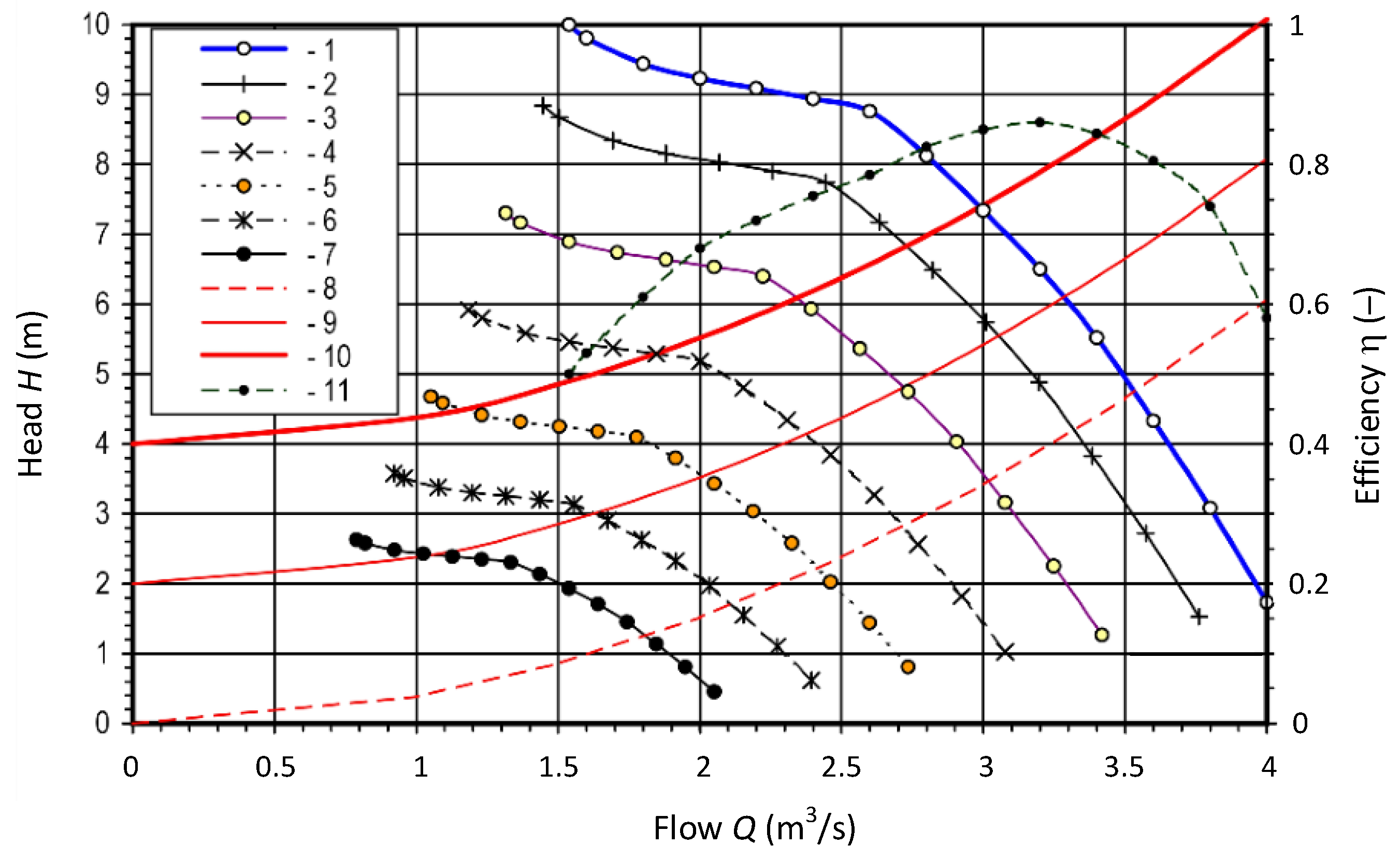
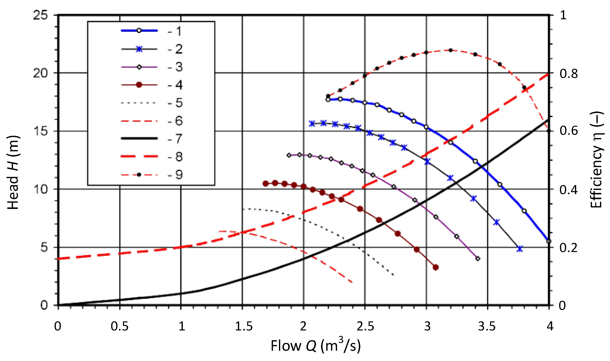
The following assumptions are made for the purpose of determining a pump’s loading torque. A pumping system, see Figure 2, pumps water from one to the other tank, both situated at the same levels, yet the distance between them is important. The dependence between efficiency and the mains and pump heads as a function of capacity is illustrated in Figure 4.

The waveforms 1–7 are plotted for the speeds: 585, 550, 500, 450, 400, 350, and 300 rpm, respectively. Waveforms 8, 9, and 10 represent the pipeline heads: H_g = 0 m; H_g = 2 m; and H_g = 4 m, and the pump’s capacity is represented with 11.

In the other case under analysis, the level difference between the tanks is taken into account. Where the geometrical head H_g > 0, the problem is solved with numerical methods. Waveforms of the rotational torque across the shaft of pump OB 16-87 working with a steel pipeline of diameter D = 1200 mm and length l = 500 m for H_g = 0 m, 2 m, and 4 m are shown in Figure 5.

An equivalent thickness of the pipeline wall irregularities is assumed as Δe = 1 mm, and total drag coefficients of the pipeline are Σζ = 1.75 [31]. Since flows in such systems can be expressed with Reynolds numbers to the order of 106, a parabolic dependence of the hydraulic resistance within the range of pipeline capacity is assumed.

In the event, the pipeline H_p equation is written as:

$$H_p=H_g+S_p{Q}^2$$

(46)

where S_p—hydraulic resistance of the pipeline.

In the simplest case of a pipeline head H_g = 0, dependences of the rotational torque M_P across the pump shaft are determined analytically as a function of rotational speed ω:

$$M_P=\frac{\mathsf{\rho }g{S}_p{Q}_o^3\hspace{0.17em}}{{\mathsf{\eta }}_o{\mathsf{\omega }}_o^3}{\mathsf{\omega }}^2$$

(47)

where ρ—water density; and Q_o, η_o, ω_o—capacity, efficiency, and rotational speed of a pump.

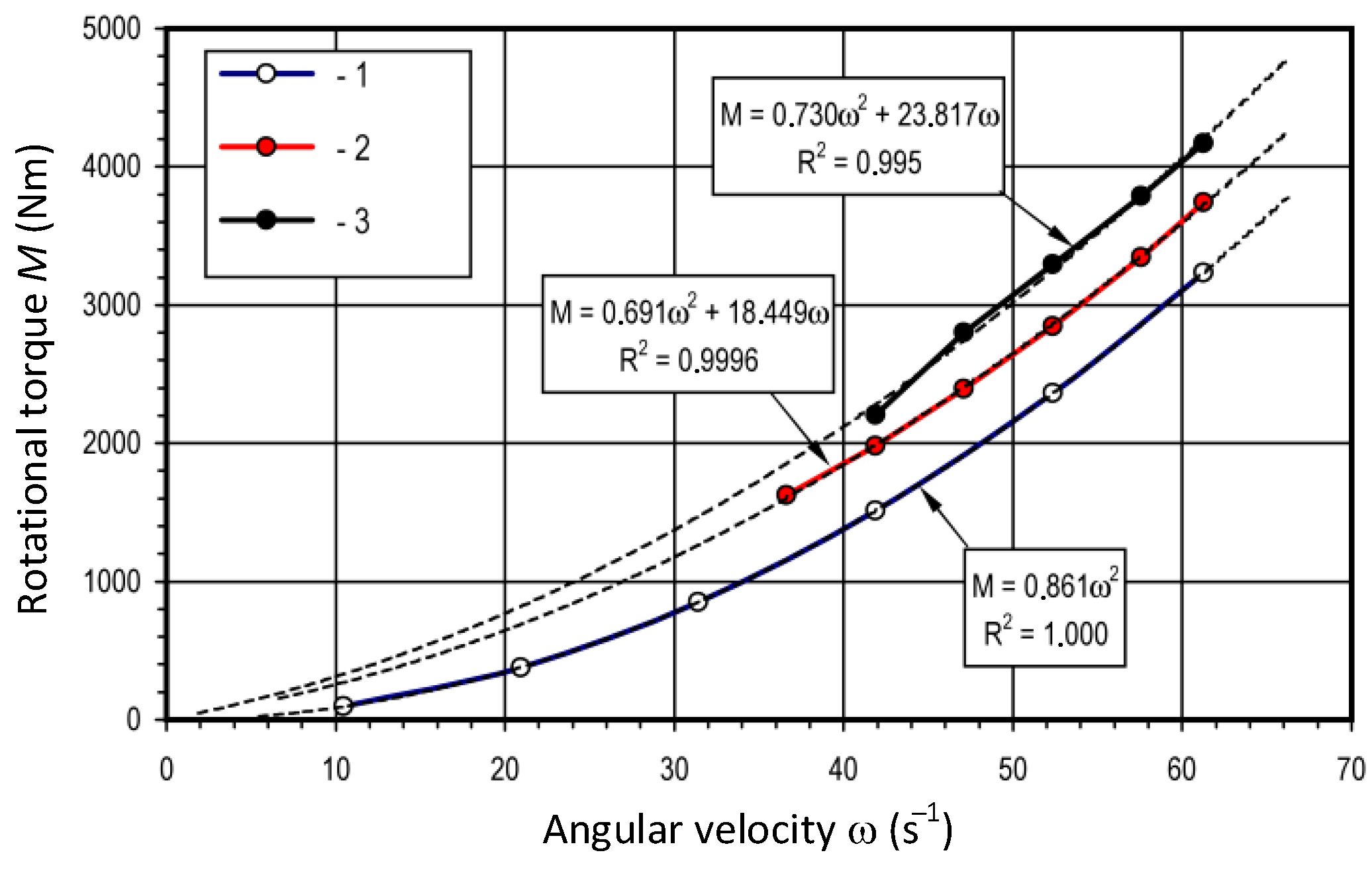
Loading torques of asynchronous drives will be based on Figure 5 as follows:

$$M_{P1}=18.449\mathsf{\omega }+0.691{\mathsf{\omega }}^2$$

(48)

$$M_{P2}=23.817\mathsf{\omega }+0.730{\mathsf{\omega }}^2$$

(49)

The method of calculating dependences for head of water and loading torques for synchronous drives is the same as for asynchronous motors. In the case of synchronous motors working with an OB 2-87 vertical pump, the waveforms of efficiency, and pipeline’s and pump’s heads as a function of efficiency, are depicted in Figure 6.

The waveforms 1–6 are plotted for speeds of: 585, 550, 500, 450, 400, and 350 rpm, respectively. Waveforms 7 and 8 illustrate the pipeline’s head for H_g = 0 m and H_g = 4 m, respectively, while the pump’s efficiency is represented with 9.

Figure 7 illustrates the dependence of the loading torque across the pump shaft on rotational speed ω at start-up of a synchronous pumping system.

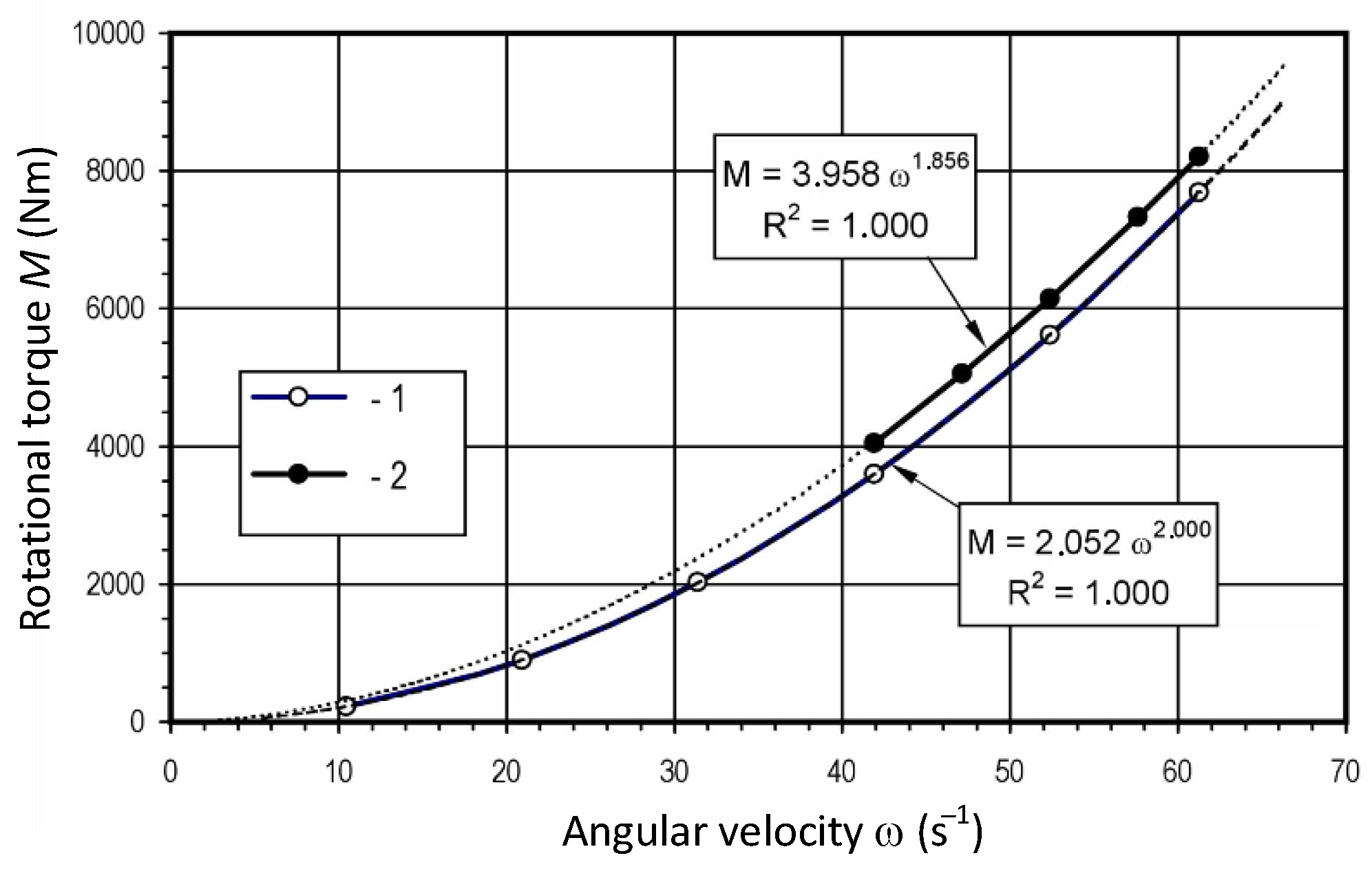
The difference between the tank levels is considered in this case. Figure 7 presents waveforms of rotational torque across OB 2-87 pump shaft working with a steel pipeline of diameter D = 1200 mm and length l = 500 m for heads H_g = 0 m and 4 m. The synchronous machine’s loading torque will be determined using Figure 7 as follows:

$$M_P=3.958{ \mathsf{\omega }}_2^{1.856}$$

(50)

The following Equations: (1), (2), (9), (10), (21), (24), (25), (34), (35), and (39)–(42) are jointly integrated considering the algebraic dependences: (3)–(8), (11)–(16), (22), (23), (26)–(33), (45), and (48)–(50).

5. Results of Computer Simulation

The computer simulation relates to the drive system whose diagram is shown in Figure 1, Figure 2 and Figure 3. Operation of two deep bar cage asynchronous motors and of one synchronous motor is shown. These are the parameters of the drive system.

• Power transformer. Type: TM-1600 (1.6 MVA; 35/6.3 kV).
• Synchronous motor: SDZB 13-52-8, P_N = 630 kW, n_N = 750 rpm; U_N = 6 kV; u_f = 42 V, p₀ = 4, J₁ = 1700 kg·m², which drives the left end of a distributed mechanical parameter shaft via a reducer gear k_T = 750/585 and the first rigid coupling SP₁, cf. Figure 2. The rotational torque is then transmitted by a long shaft with the following parameters: L = 4.5 m, D = 0.2 m, and J_P = 8.1 10¹⁰ N m and the second rigid coupling SP₂ to the input shaft of an OB 2-87 vertical pump. These are the parameters of the hydraulic system: n_N = 585 rpm, H_max = 13.6 m. Q_N = 10,700 m³/h. The pipeline details: pipe diameter D = 1.2 m, length l = 1500 m, and Hg = 4 m.
• Asynchronous drives with identical motors and motion transmissions but different heads of water lifted by vertical pumps. Motor type: 12-52-8A, P_N = 320 kW, U_N = 6 kV, I_N = 39. Parameters of the long shafts: L = 4.5 m, D = 0.15б, and J_P = 8.1 10¹⁰ N m. Vertical pump type: OB 16-87, D = 1200 mm L = 500 m, H_g = 0 m, and 4 m, Δe = 1 mm, and Σζ = 1.75.

Electromechanical analysis of transient processes proceeds as follows. The power transformer is connected to an electricity source with a rated voltage supply of 35 kV. The asynchronous drives are disconnected from the drive system; only the synchronous drive is in operation. The synchronous motor is started as the pump valve on the pipeline is closed. The excitation winding is short circuited by a low resistance. Once a sub-synchronous speed is reached, the rotor’s excitation winding is switched to a DC source and the pump valve is opened at t = 30 s. After the motor is in the synchronous state, two asynchronous drives are switched on at t = 40 s. The testing continues until the pumping drive reaches its steady state.

Three experiments are undertaken for the following excitation voltages of the synchronous motor: u_f = 12 V; 26 V; and 42 V. This corresponds to the synchronous motor operation in the following three states: asynchronous state with a resistance-inductance loading R-L, synchronous operation with a resistance loading R, cos φ = 1, and synchronous operation with a resistance-capacitance loading R-C relative to the mains, that is, an overcompensation state.

All the mechanical parameters of the three drives are converted by reducer gears to the input vertical pump shaft considering the gear k_T = 750/585. The system of ordinary differential equations is integrated by means of the fourth-order Runge–Kutta method.

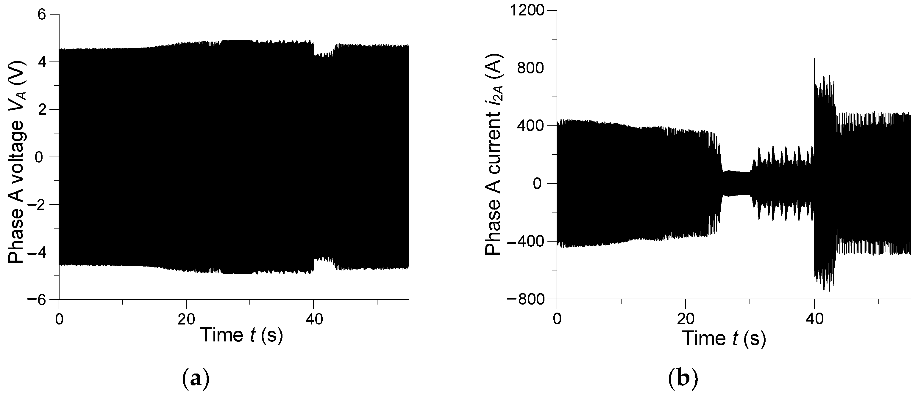
The subsequent figures show instantaneous voltage, current, and torque waveforms for the synchronous motor’s excitation voltage u_f = 12 V—experiment one.

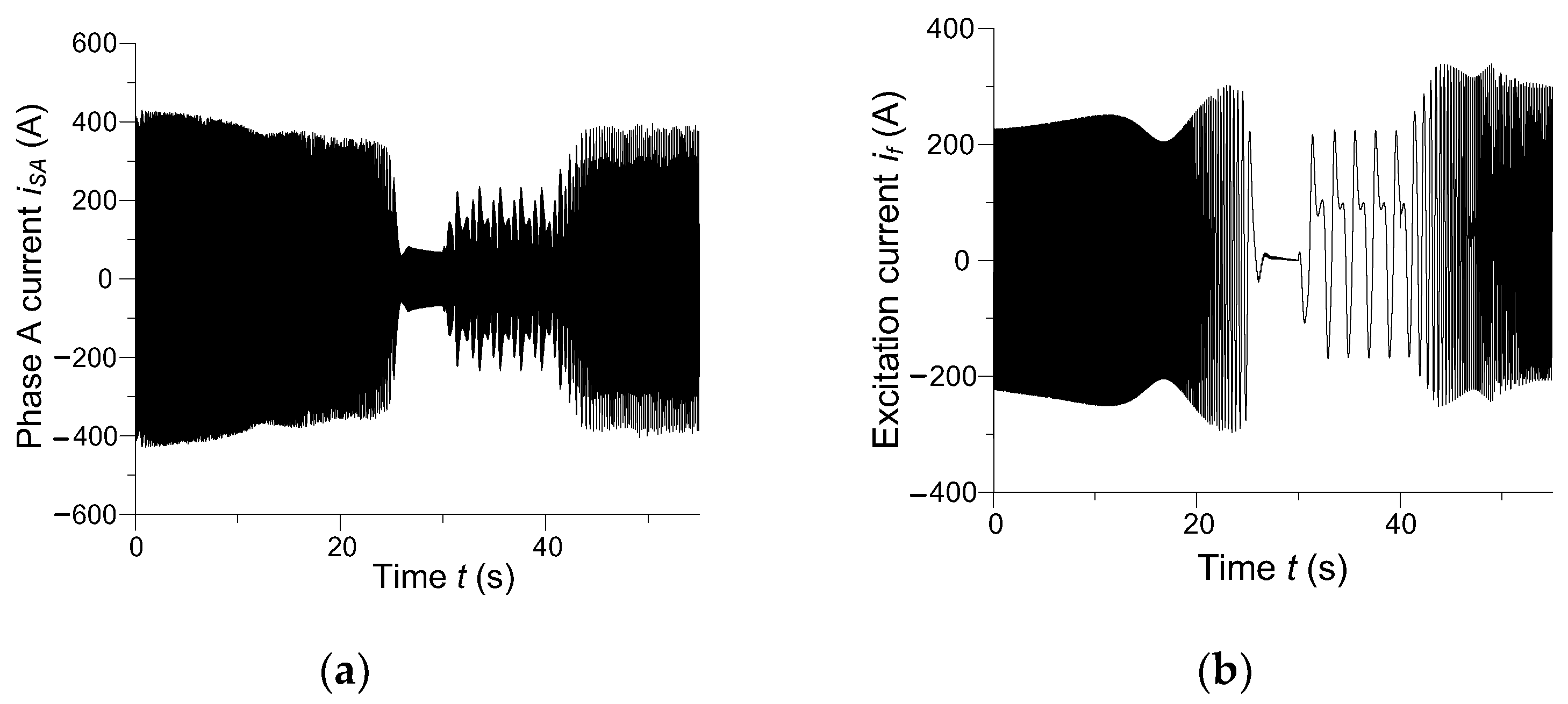
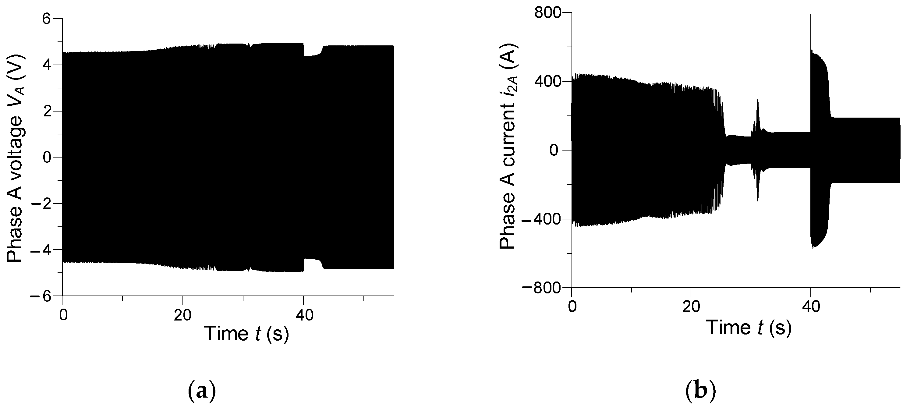
Figure 8 depicts instantaneous phase A voltage of the drive system and phase A current of the power transformer secondary winding for u_f = 12 V.

In the steady state, very high inductive currents flow across the transformer winding. The synchronous motor is fed with passive power from the mains due to the reduced excitation voltage of the rotor, which leads to the loss of synchronization and asynchronous operation of the drive. The drive system is in unstable operation, which causes high currents to flow through the secondary winding of the transformer.

Physically it is understandable. During the start-up of asynchronous drives, after the time t = 40 s, there are very high values of the magnetizing current of asynchronous motors. In addition, the synchronous motor consumes reactive power in steady state. It is obvious that this operating state is not normal for the load assembly.

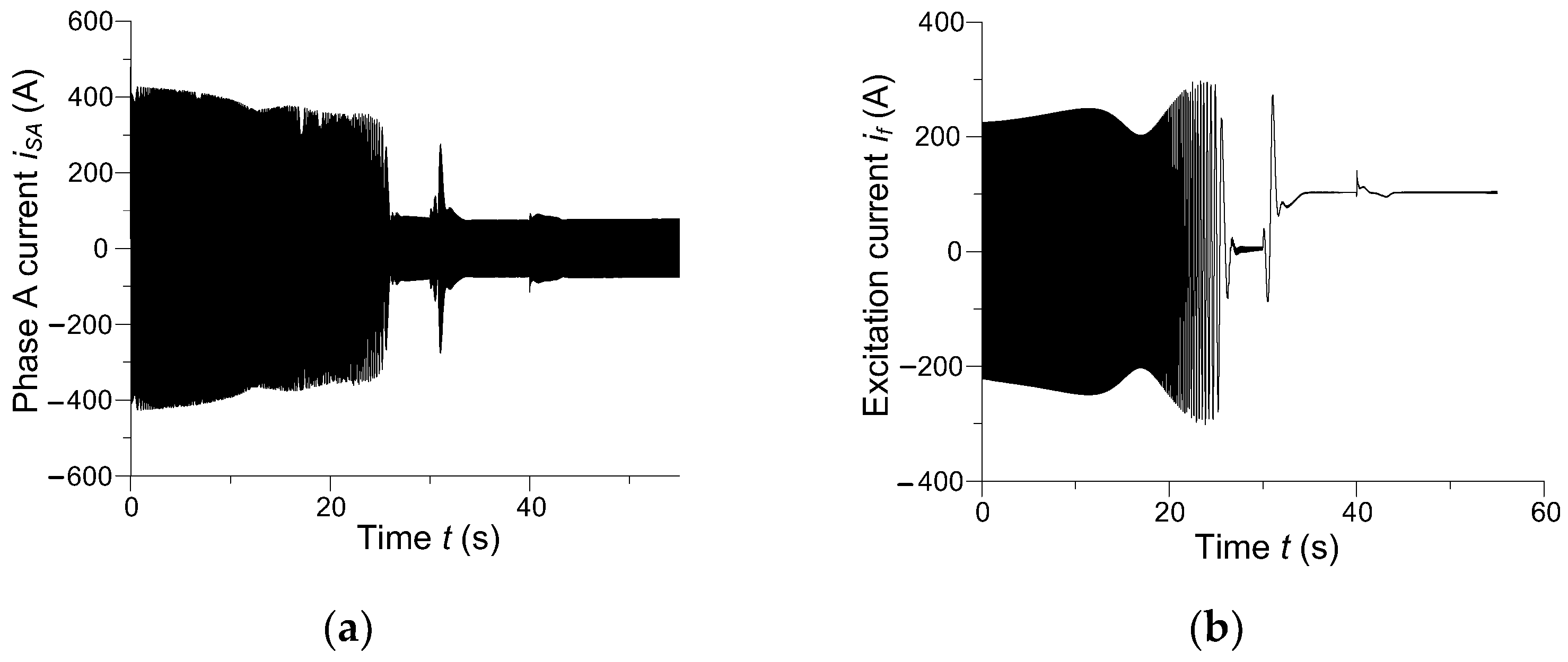
Instantaneous currents across phase A of the armature and across the excitation winding of the synchronous motor are presented in Figure 9.

In the steady state, non-periodic phase currents of enhanced amplitude flow across the armature winding, nearly three times greater than the rated current, which affirms the emergency state of the motor’s operation. The waveform of the motor’s excitation current is similar. At start-up, the excitation current is oscillatory. It should become constant in the motor’s steady state, on the other hand, which can be noted in Figure 9b. The reason for this state is that the synchronous motor is operating in an asynchronous state. Then, a slip occurs, which in turn leads to the induction of an additional alternating current component in the excitation winding. Since high-amplitude oscillatory currents flow across the excitation wiring in the steady state, the machine’s operation is certainly asynchronous. Analysis of Figure 8 and Figure 9 shows that the operation of the electric part of the drive system is incorrect.

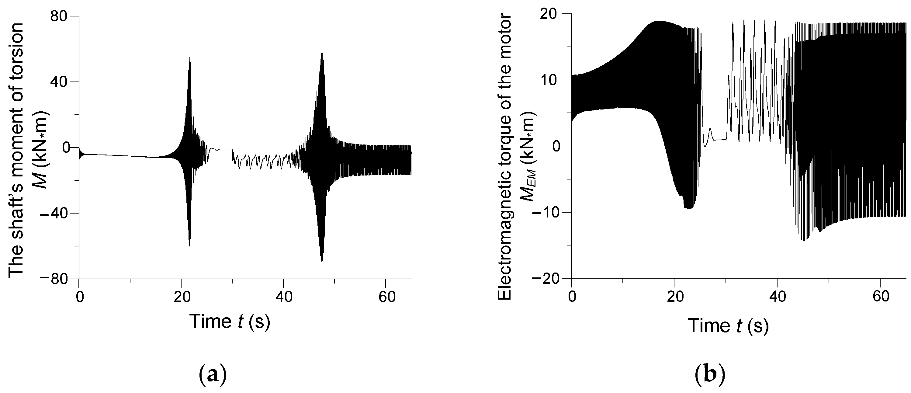
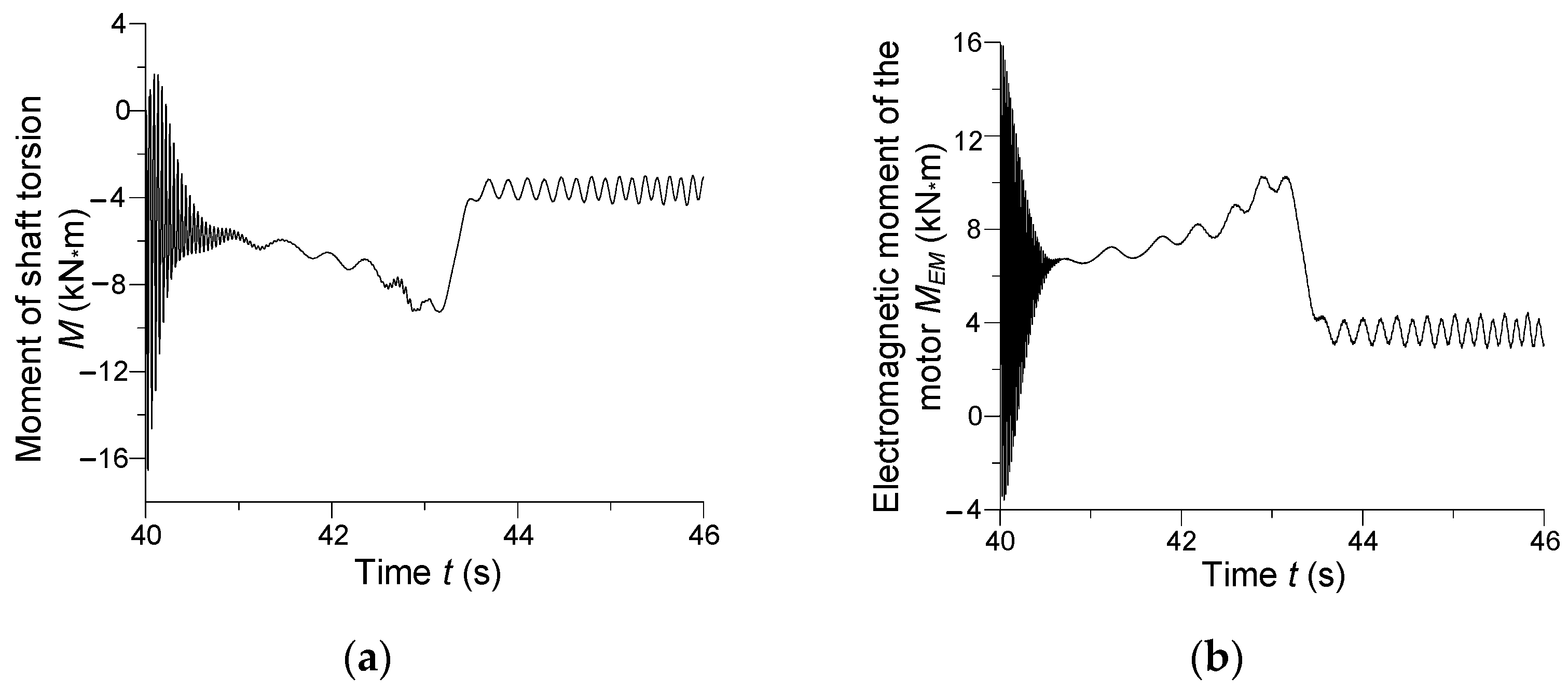
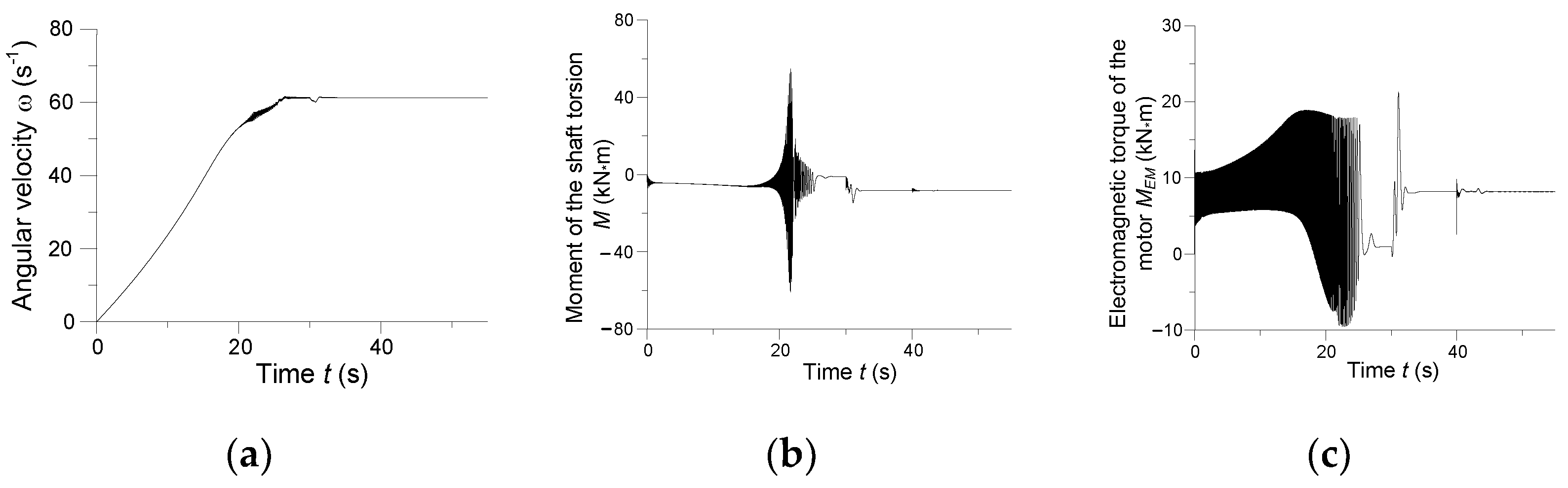
We analyse the mechanical part of the three drives. Figure 10 shows a transitional moment of torsion in the middle shaft section and electromagnetic torque of the synchronous drive.

Considering the principles of electromechanical energy conversion in a drive system, a very close connection between electromagnetic and mechanical motions is obvious. Electric drives based on susceptible transmission of motion are known to experience such dangerous phenomena as resonance or resonance-like processes (rumble, vibrations) in which the natural frequencies of the system are the same or close to the forced oscillation of the input signal. In our case of an electric drive containing a long shaft with distributed mechanical parameters, there is a problem of calculating the determined natural frequency of the drive motion transmission. Therefore, we will continue to use the term “range of natural frequencies.” By analysing the electromagnetic torque versus time it is possible to state the occurrence of oscillatory phenomena in the drive transmission of motion.

Electromagnetic torque of the motor in Figure 10b is the input signal transmitted to the mechanical section of the synchronous drive, that is, its motion transmission. For the assumed parameters of the drive system elements, the resonant frequency of the synchronous drive motion transmission is approximately 11 Hz. For these oscillations of the electromagnetic torque, resonant effects will arise in the synchronous drive, which can be noted in Figure 10a. In the time intervals t ∈ (20; 25) s and t ∈ (45; 50), synchronous drive is in resonance.

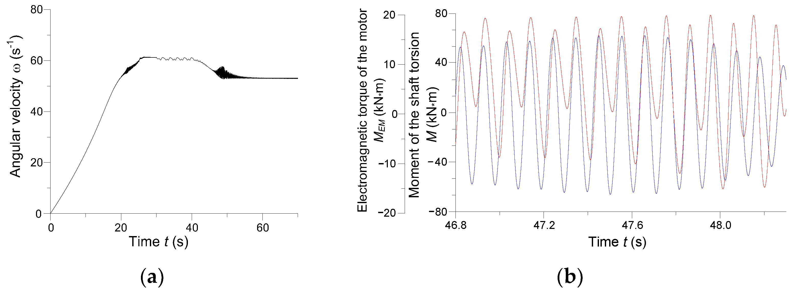
Instantaneous angular velocity of the synchronous motor rotor and the waveforms of the moment of torsion in the middle shaft section and of the electromagnetic torque of the synchronous drive are presented in Figure 11.

Instantaneous angular velocity of the synchronous motor is depicted in Figure 11a. This shows that, in the steady state, the drive operates at an asynchronous angular velocity and evidence the motor is under excited. In Figure 11b, the waveforms of moment of torsion in the middle shaft section are blue and of the electromagnetic torque of the synchronous drive are red. The resonance epicenter is within the time range t ∈ (46.8; 48.3) s. At t = 47.55 s, amplitude frequencies of the moment and the torque are virtually identical. This means the resonance reaches its maximum at that time.

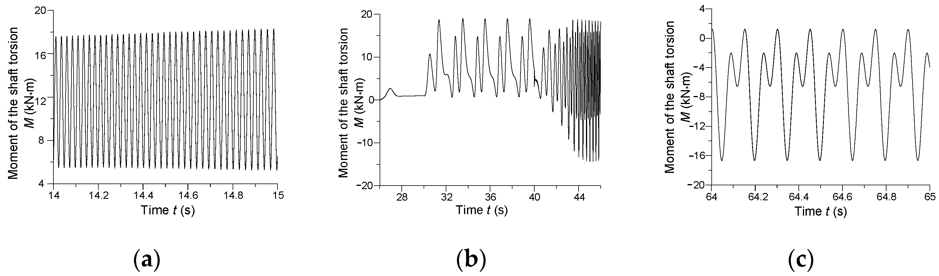
The waveforms of the synchronous drive’s moment of torsion in three-time intervals: (a)—t ∈ (14; 15) s, (b)—t ∈ (26; 46) s, and (c)—t ∈ (64; 65) s are illustrated in Figure 12.

Figure 12a demonstrates the moment’s waveform is nearly harmonic and its frequency is ca. 38 Hz, which is substantially more than the synchronous drive’s own resonant frequency of about 11 Hz. Resonance is obviously absent from the system. Figure 12b shows an essentially different situation. In the time interval t ∈ (26; 46) s, the moment of torsion’s waveform is highly non-linear. Fourier series can be used to determine the moment’s frequency. Frequencies will then vary for diverse harmonics of the moment. The first harmonic is the most important in this case. Its frequencies are of course several times lower than resonant frequency of the drive’s motion transmission. There is no resonance here, either. Steady low-amplitude resonant processes can be observed in Figure 12c. The amplitude of resonant oscillation is now around eight lower than the amplitude in the range t ∈ (46.8; 48.3) s, see Figure 10a. In this interval, oscillation frequencies cohere at higher harmonics of the moment of torsion distribution over the Fourier series.

At the time of the asynchronous start-up of synchronous drive, the frequency of electromagnetic torque varies over a rather wide range. Oscillations occur in these states too, occasionally very non-linear, which give rise to resonance at the higher harmonics of electromagnetic torque. The only advantage is that the oscillation amplitudes of electromagnetic torque are significantly lower than the amplitude of the first harmonic.

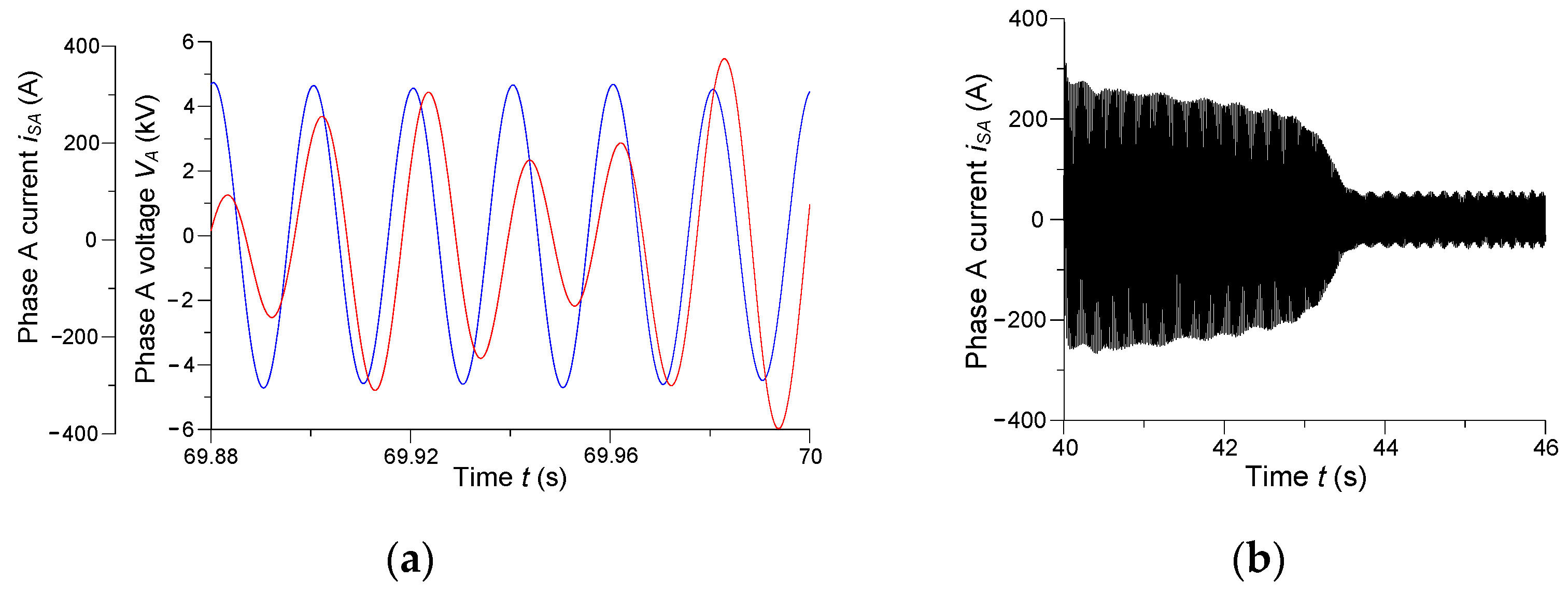
The waveforms of phase A current and voltage of the armature winding in the interval t ∈ (69.88; 70) s and of phase A current of the asynchronous motor’s stator winding in the interval t ∈ (40; 46) s are presented in Figure 13.

Figure 13a shows the operating state of the synchronous drive from the perspective of the network supplying power to the drive system. The waveform of phase A voltage is marked blue and of phase A current is red. The phase of the voltage leads the current by a significant angle of ca. φ = 50°. This corroborates the conclusion that the synchronous drive operates in an asynchronous state of under excitation.

In such a state, quite permanent transient processes are visible, which are related to the resistive–inductive load of the network.

The moment of torsion across the motion transmission shaft and electromagnetic moment in the time interval t ∈ (40; 46) s are illustrated in Figure 14.

Figure 14 demonstrates electromechanical processes in the synchronous drive, the key part of the drive system, which affects the processes in both the asynchronous drives. The waveforms of current, torque, and moment contain additional oscillations. The electromagnetic torque and the moment of torsion in the steady state are not constant, either, but oscillatory in nature.

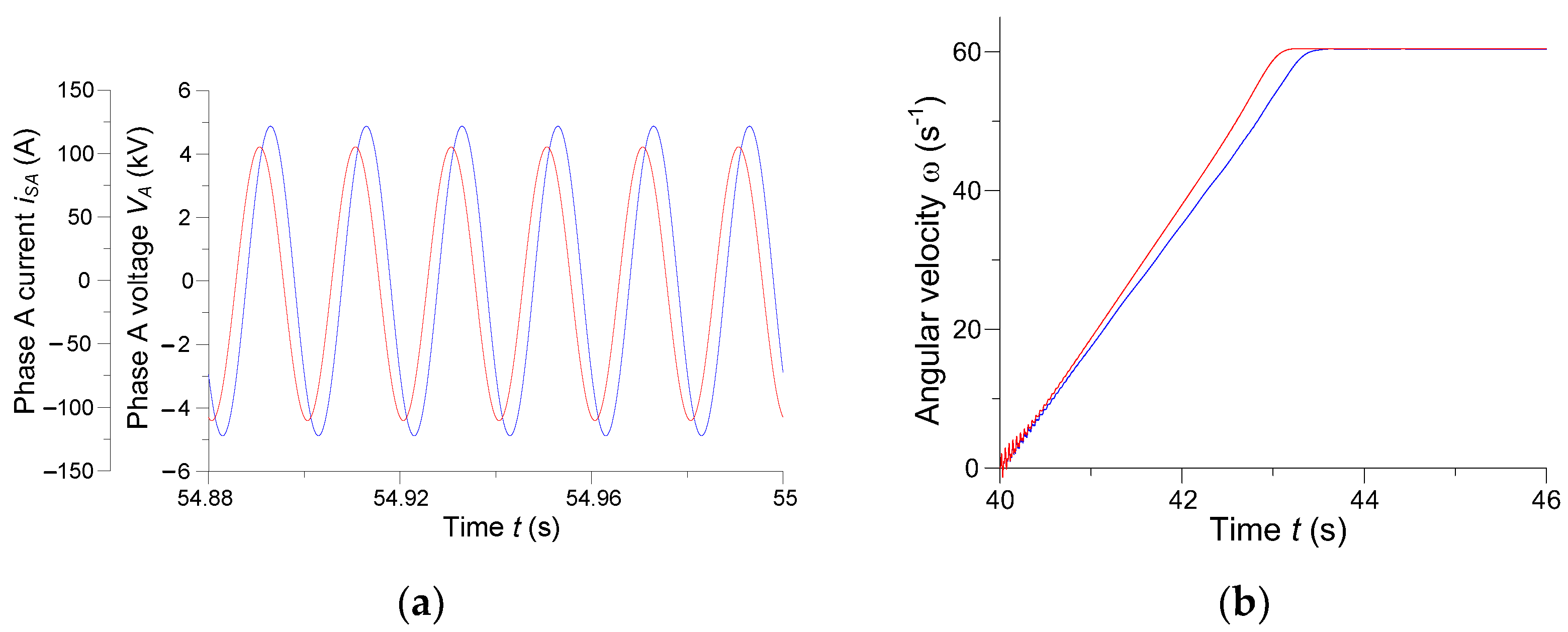
The successive figures include instantaneous waveforms of voltages, currents, torques, and moments for the synchronous motor’s excitation voltage of u_f = 26 V—the second experiment.

The instantaneous phase A voltage of the drive system and phase A current of the secondary power transformer wiring are presented in Figure 15.

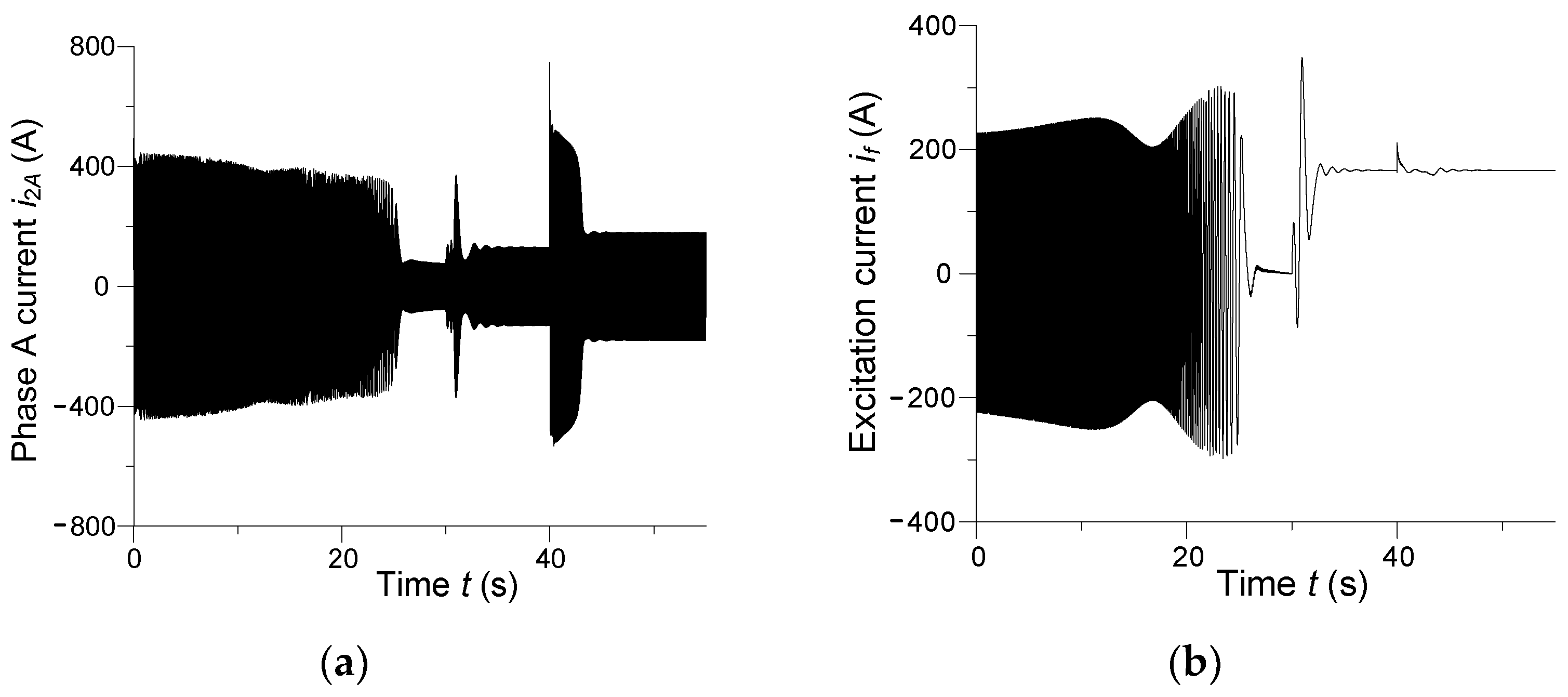
Instantaneous waveforms of phase A current of the synchronous motor’s armature wiring and excitation current are depicted in Figure 16.

A comparative analysis with the results of the first experiment (cf. Figure 8 and Figure 9) suggests a totally different operating condition of the drive system in experiment two. The synchronous drive is in a normal operating state now. The excitation voltage is selected in such a way that cos φ = 1, which means the synchronous motor only consumes the active power. The stator’s current in its steady state is sinusoid, see Figure 9a and Figure 16a. The excitation current in the steady state is constant, see Figure 9b and Figure 16b. The drive in the steady state operates at a synchronous speed, cf. Figure 11a and Figure 17a.

Figure 17a shows the instantaneous angular velocity of the synchronous drive rotor. Compared with Figure 11a, the electric drive in the steady process rotates at a synchronous speed.

The instantaneous moment of torsion in the middle shaft section and electromagnetic torque of the synchronous drive are illustrated in Figure 17b,c, which need to be compared with Figure 10. The moment of torsion across the drive shaft is exclusive of the second resonance once the excitation wiring is connected to a DC source, as the motor has become synchronous and the electromagnetic torque does not include oscillatory motions in the steady state. In addition, the moment of torsion in the steady state is constant, since the stator current is exclusive of higher harmonics and resonant processes are absent from the synchronous drive. The drive becoming synchronous substantially reduces the amplitudes of transitional shock torques and currents. It is also dependent on the motor’s excitation current.

Phase A voltage and current of the armature winding and electromagnetic torque of the first asynchronous motor are shown in Figure 18.

The voltage is blue and the current is red in the time interval t ∈ (54.88; 55) s in Figure 18a. A synchronous motor is a purely resistive load of the network, i.e., φ = 0°. We note again the stator current is sinusoid, as distinct from the first experiment, cf. Figure 13a. From the point of view of applied electrical engineering, it is related to the type of the assembly load. In the case shown in Figure 13a, the under excited synchronous motor is a resistive–inductive load on the network. According to the characteristics of the synchronous motor, the resistive–inductive load reduces the voltage of the assembly the most. However, in the case presented in Figure 18a, the situation is different—the motor is a purely resistive network load. In this case, the time constant is minimal and processes reach a steady state faster.

The instantaneous electromagnetic torque of the first asynchronous motor in the time interval t ∈ (40; 46) s is shown in Figure 18b. Compared with Figure 14b, adverse oscillatory processes are absent from asynchronous drives associated with the asynchronous operation of the synchronous drive in experiment one. Thus, both the asynchronous drives work in the normal state. Note the synchronous drives play the main role in the system under discussion. Therefore, we compare operation of the drive system to diverse operating conditions of the synchronous drive in this study. For instance, [21,24,28] address different operating conditions of susceptible motion transmission asynchronous drives that include long shafts.

The following graphs illustrate instantaneous waveforms of voltages, currents, moments, and torques for the synchronous motor’s rated excitation voltage of u_f = 42 V—experiment three.

The instantaneous phase A current across the secondary power transformer winding is shown in Figure 19a.

At u_f = 42 V, the synchronous drive works at rated excitation. The supply network is loaded with a volumetric-resistance receiver. Compared with Figure 15b, the current across the synchronous motor armature’s winding is larger in steady states. This is an example of passive power compensation by increasing the excitation current of a synchronous machine. In the final analysis, raising motor excitation current increases the voltage supplied to the drive system.

The instantaneous excitation current of the synchronous motor is shown in Figure 19b. Its waveform is similar to the one in Figure 16b. In the steady state of the second experiment (for u_f = 26 V), on the other hand, the excitation current is around i_f = 100 A, and for experiment three (u_f = 42 V), approximately i_f =180 A.

The instantaneous waveforms of phase A voltage and current across the motor armature winding are presented in Figure 20a.

The voltage is blue and the current red in the time interval t ∈ (54.88; 55) s in Figure 20a. From the perspective of the power network, the synchronous drive acts as a resistant-volumetric load with a phase shift angle of circa ϕ = −40°. The armature current is ahead of the voltage supplied to the driving motors. Instantaneous angular velocities of the first asynchronous motor’s rotor are depicted in Figure 20b, marked blue for the second experiment and red for the third.

Analysis of both of the waveforms proves operation of the drive system in the second and third experiments is correct. Owing to stabilisation, or increasing of the drive system’s voltage, the start-up time of the asynchronous drive is of course around 0.3 s shorter in the third than in the second experiment. This time difference is negligible for the practical purposes of both of the pumps’ operation. As far as the power network is concerned, the synchronous motor in the steady state generates passive power.

6. Conclusions

It is in some cases reasonable to introduce a synchronous drive to stabilise voltage in drive systems containing asynchronous drives. It helps to arrive at an absolutely rigid mechanical characteristic of a drive in the static sate, on the one hand, and to avoid adding compensation devices, for instance, static capacitor batteries, to a drive system.

Operation of synchronous drives in asynchronous states is a quite dangerous phenomenon in drive systems. In steady states, this increases currents several times compared with the rated current in the motor’s armature winding. Furthermore, it causes induction of oscillatory current waveforms in the excitation winding of a motor. Therefore, the excitation current of a motor should be calculated and adapted to all operating states of a synchronous drive as part of an electric power system.

Long elastic elements should ultimately be analysed as systems of distributed mechanical parameters for the purposes of modelling transient processes in pumping electric drives that contain complex motion transmissions including long shafts. This enables to address some latent motions that cannot always be determined, e.g., as part of the classic dual-mass interpretation of long motion transmission shafts.

During asynchronous start-up of synchronous drives with large masses of inertia, the electromagnetic torque of a motor varies its oscillation frequencies over a quite broad range. In the event, there is a risk of the motion transmission entering resonant or nearly resonant states not only for the first but also for the higher harmonics of the torque.

The results of computer simulation of transient electromechanical processes show:

• In resonant states, the moment of torsion in a drive’s motion transmission occasionally rises as much as several dozen times relative to the nominal load torque of a drive. If the susceptibility of long elastic elements of electric drives’ motion transmission are neglected and resonant motions are not addressed, a motion transmission of a drive may be wrongly selected at the stage of design.
• In asynchronous drives, the total inertia of drive motion transmission is substantially lower than in equivalent synchronous drives. In asynchronous start-up of a synchronous drive, the system is then likely to enter resonant or nearly resonant states over a quite wide time interval.
• In asynchronous operating states of synchronous drives, given low excitation currents of a motor, a system is very likely to enter a second wave of resonant oscillations whose amplitude is greater than the amplitude of oscillations in the first resonant wave.
• In asynchronous operating states of synchronous drives, contrary to synchronous states in steady states, the electromagnetic torque includes complicated oscillatory waveforms. This causes a drive to enter resonant states at the higher harmonics of the torque. The amplitude of the moment of torsion’s oscillations in the motion transmission shaft is substantially greater than the oscillation amplitude for the first harmonic of the Fourier series, which is a good development.
• Increasing the excitation current of a synchronous drive motor stabilises the drive system’s voltage and changes the nature of the synchronous drive’s load in the drive system to more resistance–volumetric loading.
• Depending on the values of excitation current, start-up times of all the drives in an electric power drive system can be regulated.

The proposed method of modelling transient processes in drive systems that contain electric load assemblies enables the analysis of transient processes not only in pumping systems, but practically in all electric drives. This makes it possible to extend the scope of our research in other branches of the economy. In our next plans, we will put into practice the simulation results that we obtained in this paper.