CBLSTM-AE: A Hybrid Deep Learning Framework for Predicting Energy Consumption

Abstract

Multisource energy data, including from distributed energy resources and its multivariate nature, necessitate the integration of robust data predictive frameworks to minimise prediction error. This work presents a hybrid deep learning framework to accurately predict the energy consumption of different building types, both commercial and domestic, spanning different countries, including Canada and the UK. Specifically, we propose architectures comprising convolutional neural network (CNN), an autoencoder (AE) with bidirectional long short-term memory (LSTM), and bidirectional LSTM BLSTM). The CNN layer extracts important features from the dataset and the AE-BLSTM and LSTM layers are used for prediction. We use the individual household electric power consumption dataset from the University of California, Irvine to compare the skillfulness of the proposed framework to the state-of-the-art frameworks. Results show performance improvement in computation time of 56% and 75.2%, and mean squared error (MSE) of 80% and 98.7% in comparison with a CNN BLSTM-based framework (EECP-CBL) and vanilla LSTM, respectively. In addition, we use various datasets from Canada and the UK to further validate the generalisation ability of the proposed framework to underfitting and overfitting, which was tested on real consumers’ smart boxes. The results show that the framework generalises well to varying data and constraints, giving an average MSE of ∼0.09 across all datasets, demonstrating its robustness to different building types, locations, weather, and load distributions.

1. Introduction

Electric power grid patterns have been impacted by the recent COVID-19 outbreak, where a typical weekday predicted demand now aligns with typical weekend days, as the workforce predominantly stays, and works from, home. This resulted in a $24\%$ measured difference between the highest and lowest weekend energy demand in Britain [1]. This unpredictable event has increased the volatility of the utility grid, by making demand forecast a difficult task. In fact, authors in [2] show that a $1\%$ increase in load forecasting error can result in a ∼GBP 10 M increase in annual operating costs [3]. Moreover, the input of several constraints, including occupant behaviours, weather conditions, price of electricity, and comfort levels aspired, combined with the surge of distributed energy resources [4,5], increased the complexity of accurately predicting energy consumption in balancing the supply and demand. Furthermore, for energy service providers to offer varying ancillary and flexible energy management services to residential and commercial buildings, accurate prediction of their energy consumption is an important requirement. This would result in cost savings and a variety of choices on the customer side, and efficient grid management on the service provider side. Other benefits include stable power supply, efficient energy balancing, efficient energy operations, and control strategies [6].

The traditional predictive algorithm for forecasting short-, medium-, and long-term demand consumption has certain limitations, such as overfitting, underfitting, short-term memory, learning from scratch, and model retraining, especially with a varied and complex dataset [7,8,9,10]. Recently, different deep learning models, such as deep neural network (DNN), including convolutional neural network (CNN) and recurrent neural network (RNN) [11,12,13,14], have been proposed for load forecasting. These studies show a general improvement of deep learning models over the traditional methods. Due to the multivariate nature of energy data involving several constraints in forecasting the load accurately, a surge in hybrid frameworks that combine two or more DNN are reported in the literature. For instance, Ref. [15] proposed an RNN and CNN architecture to predict the hourly and daily consumption of commercial buildings. In addition, Ref. [3] explored different hybrid frameworks, including LSTM/BLSTM with attention, CNN + LSTM, CNN + BLSTM, etc., for load forecasting.

However, as these models would be deployed on memory-constrained devices such as smart meters and smart boxes, the computation time is an important factor that is mostly ignored. For instance, an attention model with RNN that accounts for all hidden state vectors as opposed to other DNN and hybrid models that only account for the preceding hidden state is proposed in [3]. Although the attention model proves to be quite useful, the consideration of all the hidden states would increase the computation time which would not be suitable for lightweight and memory-constrained devices as applied to the case in hand. Moreover, as it has been well established that environmental conditions and occupants’ behaviour greatly impact the accuracy of load forecasting errors [16,17], the hybrid frameworks did not examine these factors on their proposed models. Likewise, as DNN-based predictive models could be highly unstable due to several dynamics in the data, the proposed models in [7,18,19] only consider residential energy prediction without ascertaining the generalisation of their model to varying datasets and dynamics.

Thus, to solve the three identified challenges above, this study proposed a hybrid deep learning framework—CBLSTM-AE, particularly, a deep CNN and an autoencoder (AE) with BLSTM as the encoder and LSTM as the decoder. The CNN layers extract important features from the dataset, and the integrated AE is for feature representational learning through the BLSTM and LSTM layers. The BLSTM uses forward and backward directions to make a prediction, then output to an LSTM-AE layer to decode before final output to two fully connected layers prior to the final predicted output. Secondly, several constraints that impair the accuracy of ECPs are considered in the proposed framework. Finally, we tested the generalisation of our framework on varying energy users to include SMEs, households, and universities in Canada and the UK, utilising various lengths of data.

The contributions of this work is as follows:

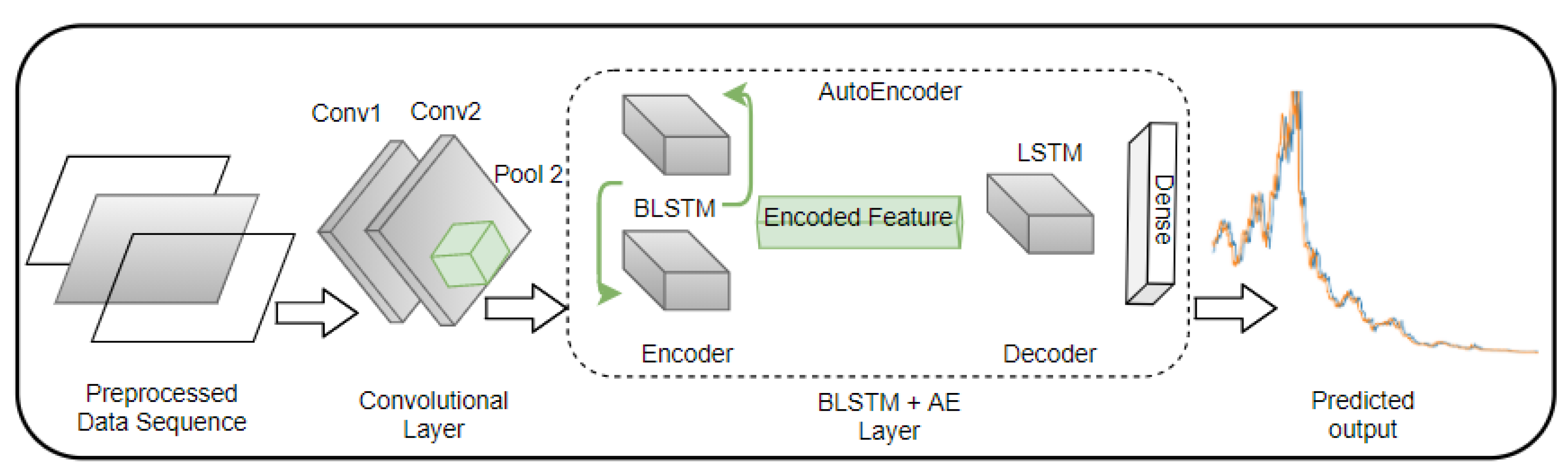
• We proposed a hybrid deep learning architecture comprising two CNN layers and an AE with BLSTM as the encoding layer and LSTM as the decoding layer for load forecasting of real energy consumers.
• Peak load varies among buildings and countries, resulting in a poor generalisation of DNN models. Thus, the generalisation ability of the framework is tested using a varied length of datasets across households and SMEs over two different countries—the UK and Canada.
• As energy consumption prediction (ECP) can be greatly impacted by irregular occupant behaviours, weather uncertainties, and the nonlinearity of building dynamics [20,21,22,23], the impact of these dynamics was not addressed in [7,18,19]. Thus, this work explores the effect of weather and weekly index in the proposed framework.
• As other authors, including [7,18], proposed hybrid deep learning but with high computation time, our proposed architecture achieved a $56\%$ reduced computing time which is of importance as the algorithm is being tested on energy consumers’ memory-constrained smart boxes.

The remaining sections are organised as follows. Section 2 reviews the energy prediction frameworks discussed in the literature. Section 3 presents the details of the proposed CBLSTM-AE framework and its algorithm. Section 4 evaluates the proposed CBLSTM-AE, while Section 5 discusses the result of the CBLSTM-AE. Finally, Section 6 concludes the paper with future work.

2. Literature Review

In the past, ECP has been achieved using statistical machine learning (ML) methods and an alternate ML method, as proposed in [24] utilising a cuckoo search algorithm by means of Levy flights, to forecast electricity consumption for the organisation of petroleum exporting countries. Some statistical ML utilised for ECP includes random forest [16], multiple linear regression [17], gradient boosting [17], support vector regression [17,25], etc. Although these models have their strengths in predicting energy consumption, the multivariate time series nature of ECP and the irregular trends and seasonal patterns of data render the traditional statistical ML ineffective in accurately predicting energy consumption [8,26]. On the contrary, recent research contributions seem to be adopting deep learning frameworks for ECP. For instance, Ref. [27] used a feedforward and backpropagation neural network with an improved version proposed in [28] using a deep extreme learning machine. A recurrent inception CNN (RICNN) is proposed in [14] for ECP using an RNN and 1-dimensional convolution inception module to consider the effect of the hidden state vector values and the prediction time from closer time steps. Authors in [29] adopted a stacked AE to extract relevant features by reducing randomness and noisy disturbance in the load data. However, the deep learning frameworks experience difficulty in spatial–temporal features of load data modelling [7].

Thus, recent works proposed a hybrid approach of two or more DNNs in modelling the spatial–temporal features inherent in load forecast data. These works include LSTM and genetic algorithm [30], LSTM and particle swarm optimisation [31], CNN and LSTM framework [7], and CNN with BLSTM [18]. In [19], the authors proposed CNN and multilayer BLSTM for short-term prediction, where the sequence of refined data is fed into the CNN via the multilayer BLSTM network to learn the sequence pattern effectively using the forward and backward direction of BLSTM. In [7,18], the CNN layer is used to extract spatial features and the LSTM and BLSTM layers to model the temporal features to make the ECP predictions using the individual household electric power consumption (IHEPC) dataset [32]. The result obtained in [7] confirmed that the CNN-LSTM predicts the local features of the time series better than the linear regression method. This achieved better performance compared to the traditional methods, with a mean square error (MSE) of $0.37$. Likewise, the result obtained in [18] was compared to [7] and the linear regression method, which outperformed both methods with an average MSE of $0.06$ for the IHEPC daily dataset.

Although these hybrid frameworks can predict the spatial correlation of multivariate time series data with irregular time information of load data, their loss function, which is the difference between the actual and predicted value, is high. Thus, a framework to correctly predict the energy consumption data with minimal error and computation time is needed, as an application on real smart meters is limited in the literature. The employed frameworks and study objectives are summarised in

Table 1. Comparative summary of prediction frameworks for energy consumption.

Prediction Models	Ref.	Year	Method	Period	Description
Statistical Models	[16]	2018	Random forest	Hourly, monthly, yearly	Hourly building energy prediction using trained RF with different parameter tuning. They also investigated the impact of behaviour changes on prediction accuracy.
	[17]	2017	Multiple LR, RF, gradient boosting	-	Discussed feature filtering and ranking using different statistical modelling.
Machine Learning Models	[27]	2019	Neural network	Short-term: hourly, day, weekly	Proposed a feedforward backpropagation neural network on energy consumption data with statistical moments.
	[25]	2019	SVR	Hourly	A vector field-based SVR for ECP is proposed by approximating the high nonlinearity between input and output to linearity.
Deep Learning Models	[28]	2018	Deep extreme learning machine	Weekly, monthly	The authors explored deep extreme learning machine (DELM), adaptive neuro-fuzzy inference system (ANFIS), and ANN. They proposed DELM for ECP due to its performance over ANN and ANFIS.
	[33]	2017	Pooling-based DRNN	-	Addresses overfitting forecasting performance using a pooling-based DRNN, testing their solution on real smart meters in Ireland.
Hybrid Models	[7]	2019	CNN-LSTM	Short and medium-term	CNNs for spatial features extraction and LSTM for temporal features modelling.
	[18]	2019	CNN-BLSTM (EECP-CBL)	Short, medium and long-term	CNNs for spatial features extraction and BLSTM for features modelling for final prediction.
	[14]	2019	RICNN	48 time steps, 30 min interval	Integrate RNN and 1-D convolution inception module to calibrate hidden state vector values and prediction time.
	[34]	2020	AE and SOM	-	Deep AE for representational learning with result fed into an adaptive self-organizing map (SOM) clustering algorithm, before performing a statistical analysis on the obtained clustered data for prediction.
This study		2021	CBLSTM-AE	30 min interval and 24 h	Proposed a hybrid architecture of CNN with an AE-BLSTM as the encoder and LSTM as the decoder to correctly predict electricity consumption, while testing the generalisation ability on various datasets in a real environment.

, which also compares the literature with this work.

3. Proposed Framework (CBLSTM-AE)

This section presents the proposed framework for ECP. The data cleaning method to deal with missing values is first presented alongside a rolling window method for improved performance.

3.1. Data Cleaning and Rolling Window

The dataset is collected through the smart meters of the consumers (households and SMEs). Sometimes, there are missing data points majorly due to network failure including climate, measurement errors, and metering problems. Smoothing filters, including locally estimated scatterplot smoothing (LOESS), locally weighted SS (LOWESS), robust versions of LOESS and LOWESS (RLOESS, RLOWESS), or moving average filter [19,28] are utilised for data cleaning. In this study, to remove noise from the data for effective forecasting/accurate result, depending on the time resolution, we utilised the previous set of observations (day, week, month, or year) and a moving average filter [19,35] calculated by a rolling window.

A rolling time window algorithm is utilised to increase the dexterity of the predictive framework, where a mapping function is developed over a training set. The developed mapping function is then used for subsequent forecasting. For instance, in (1), if x represents a set of past data points, i.e., $x=\left(y\right[t-l],\cdots ,y[t-l+h\left]\right)$, we develop a mapping function x to $y\left(t\right)$ over training data points, then use the developed mapping function for subsequent forecasting. This method allows the time dynamics of data to be considered which is highly needed in these uncertain times for accurate prediction.

$$y\left(t\right)=F\left(x\right)$$

(1)

In this case, we used a rolling subset of the data for faster training as the framework will be run on consumers’ memory-constrained devices (smart boxes). In addition, the dataset is normalised, i.e., brought into a given data range to present the same data range for all samples. A detailed analysis of different normalisation techniques is discussed in [8], where the results suggested that the standard transform normalisation technique outperformed other techniques because it scales and centres each feature of the data independently. Thus, a standard transform normalisation technique is applied in this study.

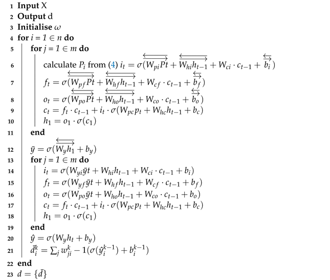
3.2. Proposed CBLSTM-AE

The proposed ECP framework is illustrated in Figure 1. The framework consists of multiple architectures including two CNN layers and an AE architecture made up of a BLSTM as the encoder and a single LSTM layer as the decoder.

3.2.1. CNN

CNN is especially skillful at extracting complex features and can store varied irregular trends. The extraction of complex features reduces the parameters needed for making predictions, thus reducing the network computations while machinating accuracy. The CNN utilises a weight distribution concept in nonlinear problems such as ECP. CNN has hidden layers consisting of a pooling layer, convolution layer, and an activation function. The convolution layer is applied to the input data to convert it into a features map. Then the pooling layer samples the features map to extract high-level convolution features, thereby reducing the dimension of the features map. The feature extraction of CNN and its downsampling process reduces the computation time, making it ideally suitable for the proposed application. In the proposed architecture, the CNN layer receives eight input constraint variables impacting correctly predicting energy consumption, including weather conditions (temperature, humidity, wind speed, and dew point) and week index (weekday, weekend, and bank holiday). These are further processed through the hidden layers to produce an output ready for the AE architecture.

3.2.2. BLSTM-AE

The output of the CNN layer is fed into the input of the BLSTM, which also serves as the input to the AE layer. While CNN extracts important features from the dataset, the BLSTM-AE layer is for information analysis and sequence prediction. The vanilla LSTM architecture is an enhanced version of RNN to overcome its vanishing gradient problem by using memory cells and gates (input, forget, and output). The input gate determines the input data to be reserved, the forget gate determines the data to be discarded, and the memory cells store the processing states, while the output from the LSTM is delivered by the output gate. However, LSTM only considers the previous state of information, thereby losing valuable information from the next state. Thus, a BLSTM is used to combine the information in the sequence prediction in both forward and backward directions. AE, on the other hand, is specially designed for representation learning, to understand unsupervised inputs in a feature vector. It consists of an encoder and a decoder to first encode the input sequence before subsequently decoding it using internal representations. Thus, the BLSTM-AE learns the temporal dependencies of the dataset from one sequence to another, positively impacting the predicted output.

3.2.3. LSTM-AE

To reduce the complexity of the proposed architecture, a single LSTM is utilised at the AE decoder as opposed to the BLSTM of the encoder. The single LSTM is also capable of learning from temporal dependencies from one sequence to another. The encoded information from the output of the BLSTM-AE is decoded by the single layer of LSTM-AE before proceeding to two fully connected layers for the final predicted output. The mathematical formulations of the proposed architecture are summarised as follows.

Given the input vectors $x_i^m=\{x_1,x_2,\cdots ,x_n\}$, where $x^m$ represents the varied input vectors, including energy consumption, weather data, week index, etc., of $m\in M$, and n is the number of normalised 30 min unit per window of observation, feeding the input vector ${x_i}^m$ into the CNN layer, the resulting output is expressed in Equation (2).

$$y_{ij}^m=\sigma (b_j^m+\sum _{m=1}^M{w}_{m,j}^1{x}_{i+m-1,j}^0)$$

(2)

where $y_{ij}^m$ resulted from the output vector $x_{ij}^m$ of the previous layer. $b_j^m$ is the bias for the jth feature map, m is the index value of the filter, w is the weight of the kernel, and $\sigma$ is the activation function for the CNN. Equation (3) is the output vector for the kth convolutional layer, in this case, the second convolutional layer in our framework.

$$y_{ij}^{m\left(k\right)}=\sigma (b_j^{m(k)}+\sum _{m=1}^M{w}_{m,j}^{m\left(k\right)}{x}_{i+m-1,j}^0)$$

(3)

The pooling layer of the convolutional layer downsamples the activation from feature maps to reduce the number of parameters and network computation costs. The max-pooling layer represented by (4) uses the maximum value from the previous layer for its downsampling, which also helps in adjusting model overfitting [7].

$$P_{ij}^{m\left(k\right)}=\underset{r\in R}{max}{y}_{i\times T+rj}^{k-1}$$

(4)

where y represents the pooling size and T is the stride deciding the length of the input data.

The output from the maximum pooling layer is fed to the input of the BLSTM layer through the gate units. BLSTM consists of different gate functions (input, output, and forget gate) in backward and forward directions, and each gate is activated when the memory cells update their states, represented in (5) through (7).

$$i_t=\sigma (W_{piPt}+W_{hi}{h}_{t-1}+W_{ci}·c_{t-1}+b_i)$$

(5)

$$f_t=\sigma (W_{pfPt}+W_{hf}{h}_{t-1}+W_{cf}·c_{t-1}+b_f)$$

(6)

$$o_t=\sigma (W_{poPt}+W_{ho}{h}_{t-1}+W_{co}·c_t+b_o)$$

(7)

where $\sigma$ is the activation function, b is the bias, and $c_t$ is the cell state. $P_t$ is the output of the max-pooling layer at time t that contains the critical energy consumption data and other variables used as the input to the AE via the BLSTM layer. $i_t$, $f_t$, and $o_t$ are the input, forget, and output gate, respectively. $h_t$ is the hidden state of the BLSTM cell, which is updated at every t step in both forward and backward directions. The hidden state and cell state determined through the gate operation of the BLSTM is expressed in (8) and (9) for the cell and hidden state, respectively.

$$c_t=f_t·c_{t-1}+i_t·\sigma (W_{pc}{p}_t+W_{hc}{h}_{t-1}+b_c)$$

(8)

$$h_t=o_t·\sigma \left(c_t\right)$$

(9)

The output of the BLSTM layer is concatenated for both forward and backward direction, expressed as

$$\overline{y}=\sigma (\overleftarrow{\overrightarrow{W_y{h}_t}}+b_y)$$

(10)

The output of the BLSTM $\overline{y}$ is fed as the input of the decoding LSTM, where the resulting output $\widehat{y}=\sigma (W_y{h}_t+b_y)$ represents the input to the two fully connected dense layers expressed in (11) for the final predicted output.

$$d_i^k=\sum _j{w}_{ji}^k-1(\sigma \left({\widehat{y}}_i^{k-1}\right)+b_i^{k-1})$$

(11)

To sum, the CNN layer extract spatial features from the input data, and the BLSTM-AE accepts the features from the CNN to learn temporal dependencies from between sequences for a convincing predicted output. The proposed CBLSTM algorithm is presented in Algorithm 1.

Algorithm 1: CBLSTM-AE Algorithm.

4. Framework Evaluation

This section presents the experimental setup, dataset description, and evaluation metrics for the proposed framework.

4.1. Dataset Description

To evaluate the effectiveness of our framework against the state-of-the-art, we first used the available UCI dataset [32], before applying the framework to our dataset for predicting the demand consumption on Q-Energy platform (Q-Energy platform is a UK-based digital energy services provider, helping customers reduce their energy costs, carbon footprint, and operational risk by proactively managing their energy usage, generation, and storage of energy). To avoid repetition, a detailed description of the UCI dataset is provided in [7,8,18]. For the Q-Energy platform, we used SMEs and household data from both the UK and Canada. Specifically,

Table 2. Dataset demography.

Building Name	Average Demand (kWh)	Data Length (Weeks)	Building Type	Occupancy	Location
Hospital	13,306.99	144	Hospital	∼450	UK
Office	$1793.16$	92	SME	∼30	Canada
Restaurant	$101.69$	71	SME	∼60	UK
Carehome	$158.44$	69	Residential	∼30	UK
MMU	$9071.89$	260	University	∼400	UK

summarises the dataset demographics. For the Hospital and Carehome data, the occupancy includes the bed space and the staff, while the Restaurant includes the staff and customers at peak period. The multivariate data consists of weather conditions (temperature, humidity, wind speed, and dew point), week index (weekday, weekend, and bank holiday), and the actual consumption data of 30 min resolution over different data lengths. The impact of COVID-19 increased the importance of a week index because a typical weekday is now a weekend, as people work from home. In addition, the effect of different lengths of data impacts the accuracy and generalisation of the predictive framework, which is further discussed in the results section.

The UCI dataset is similar to the private dataset used in this study. Both datasets have eight input variables and one output target, but different constraints. The UCI dataset has a total of 2,075,269 records with 25,979 missing values which are handled in the data cleaning step of the proposed CBLSTM-AE framework. The UCI dataset is for residential buildings while the private datasets are for residential, SMEs, and university. We converted the time resolution of both datasets to 24 h for short-term electricity prediction.

4.2. Experimental Setup and Evaluation Metrics

The computation to train and test the developed framework is performed on Google Colaboratory [36] using Intel Core i7-CPU, 16 GB RAM, and 64-bit operating system. After extensive experimentation and analysis of different parameters, the hyperparameter values meeting the optimal performance of the proposed framework discussed in Section 3.2 for the use case are chosen and are summarised in

Table 3. The proposed CBLSTM-AE and its definition.

No.	Layer Type	Neurons	Param
1	Input	8	8
2	Convolution1D	64	1600
3	Convolution1D	64	12,352
4	MaxPooling1D	64	0
5	Bidirectional	128	66,048
6	Flatten	128	0
7	Repeat vector	128	0
8	LSTM	64	49,408
9	TimeDistributed (Dense)	32	2080
10	TimeDistributed (Dense)	1	33

. After further extensive experiments, we selected Adam optimiser, a learning rate of $0.001$, 70 epoch, 160 batch-size, $0.33$ validation split, and ReLU activation function. Particularly, the ReLU activation function is less sensitive to random initialisation, making it stable. ReLU’s gradient does not saturate, and it runs great on low-precision hardware, resulting in easy computation of its gradient.

We evaluated the performance of the proposed framework using MSE, mean absolute error (MAE), root mean squared error (RMSE), and the computation time. The computation time includes the training and testing time of the framework on the different datasets. The MSE measures the average of the squares of the difference between the predicted and actual values illustrated in (12):

$$\mathrm{MSE}=\frac{1}{n}\sum _1^n{(y-\overline{y})}^2$$

(12)

where $\overline{y}$ is the vector of n predictions produced from the n energy consumption dataset, and y is the observed vector of the predicted energy consumption variables. RMSE expressed in (13) is the standard deviation of predicted errors, i.e., the root mean square of MSE:

$$\mathrm{RMSE}=\sqrt{\frac{1}{n}\sum _1^n{(y-\overline{y})}^2}$$

(13)

On the other hand, MAE expressed in (14) measures the absolute differences between the predicted and the actual values:

$$\mathrm{MAE}=\frac{1}{n}\sum _1^n|y-\overline{y}|$$

(14)

5. Results and Discussion

In this section, an experiment to select an appropriate input value for the rolling window is first presented. Then, a comparison against the state of the art using the UCI dataset is first presented. Then, the generalisation of the proposed framework to a different dataset is presented, closely followed by the performance analysis of the relationship of different datasets length to the proposed framework.

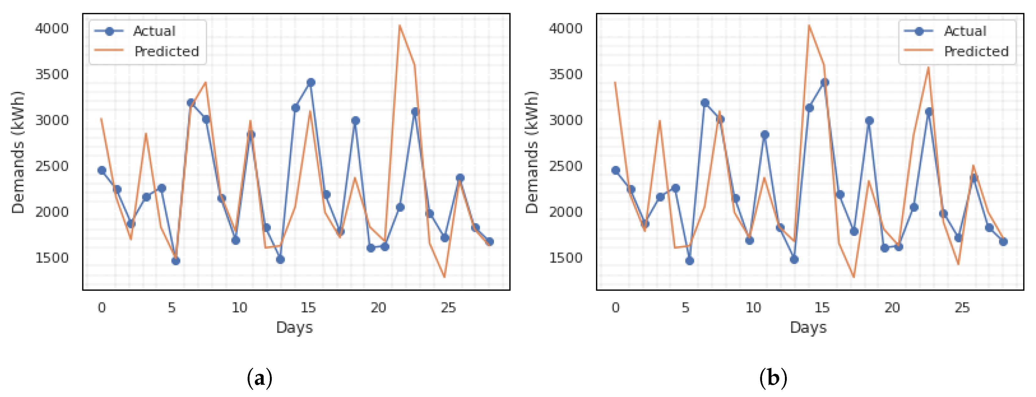
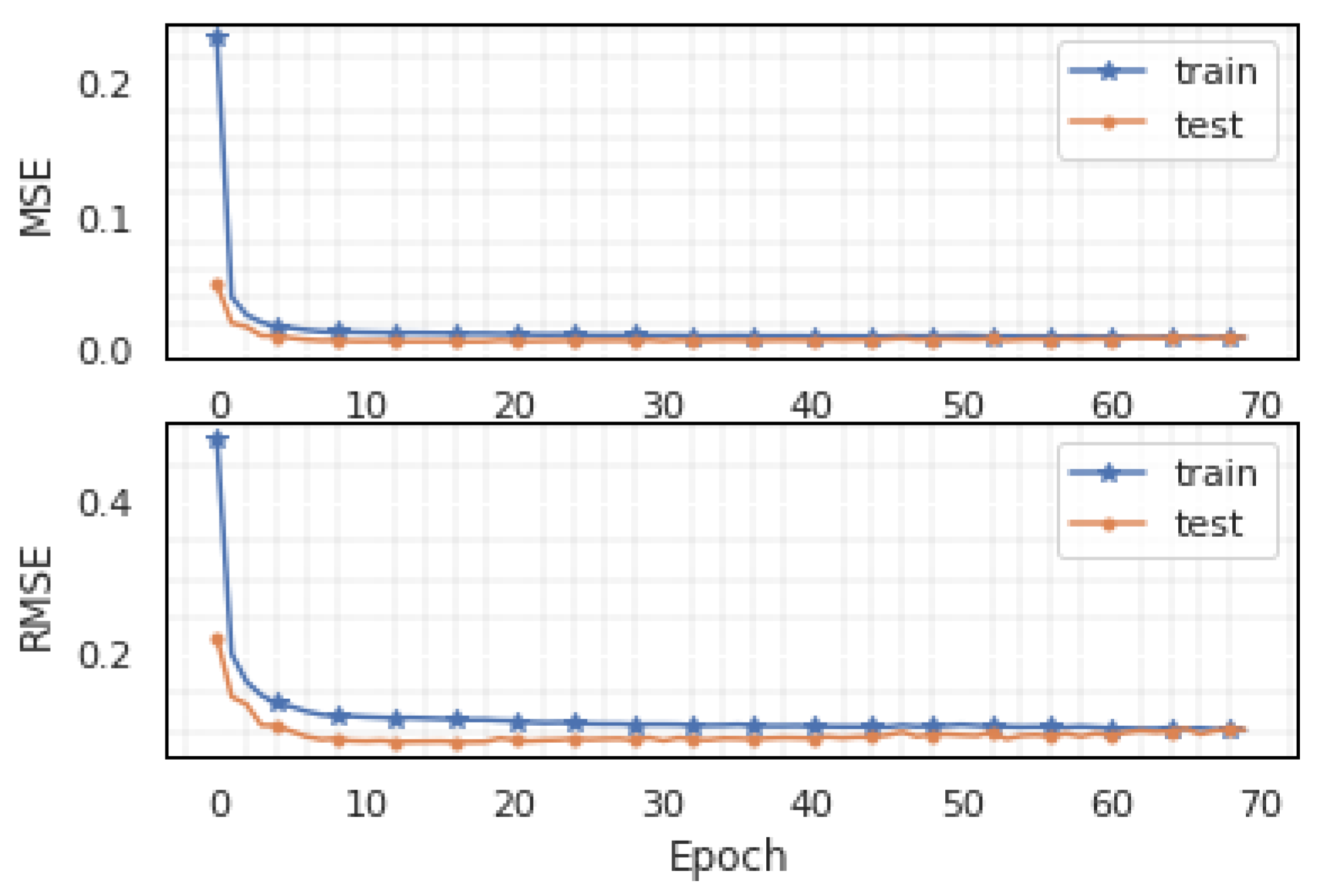
5.1. Experiment on Rolling Window Input

Rolling window analysis of time-series data assesses the stability and forecast accuracy of the model. In the rolling window analysis discussed in Section 3.1, the input data x of past observation points affect the accuracy of the model. For instance, to make a weekly prediction, the actual data of a previous observation is made available as input into the model. This allows the model to utilise the best available data for prediction. We performed different experiments in selecting an optimal input size for the model. This is illustrated in Figure 2. The 30 min smart meter data for the evaluation is reprocessed to daily data for a month forecast. To predict 4 weeks data, Figure 2 shows the experiment results of using different an input sizes, including 7 days, 14 days, 21 days, and 28 days, respectively. For the daily data ECP, the difference between the actual and predicted values shown in Figure 2 for a 28-day prediction is very narrow with a good fitting for Figure 2a,b. The accuracy of the predicted vs. actual fitting decreases as the input size increases. In addition, the computation time increases as the window size increases. However, utilising the defined evaluation metrics, input size of 14 achieves the lowest loss value. Figure 3 shows an example of the training and validation loss function of the UCI dataset for MSE and RMSE, respectively, for input size 14 which is selected to evaluate the proposed framework.

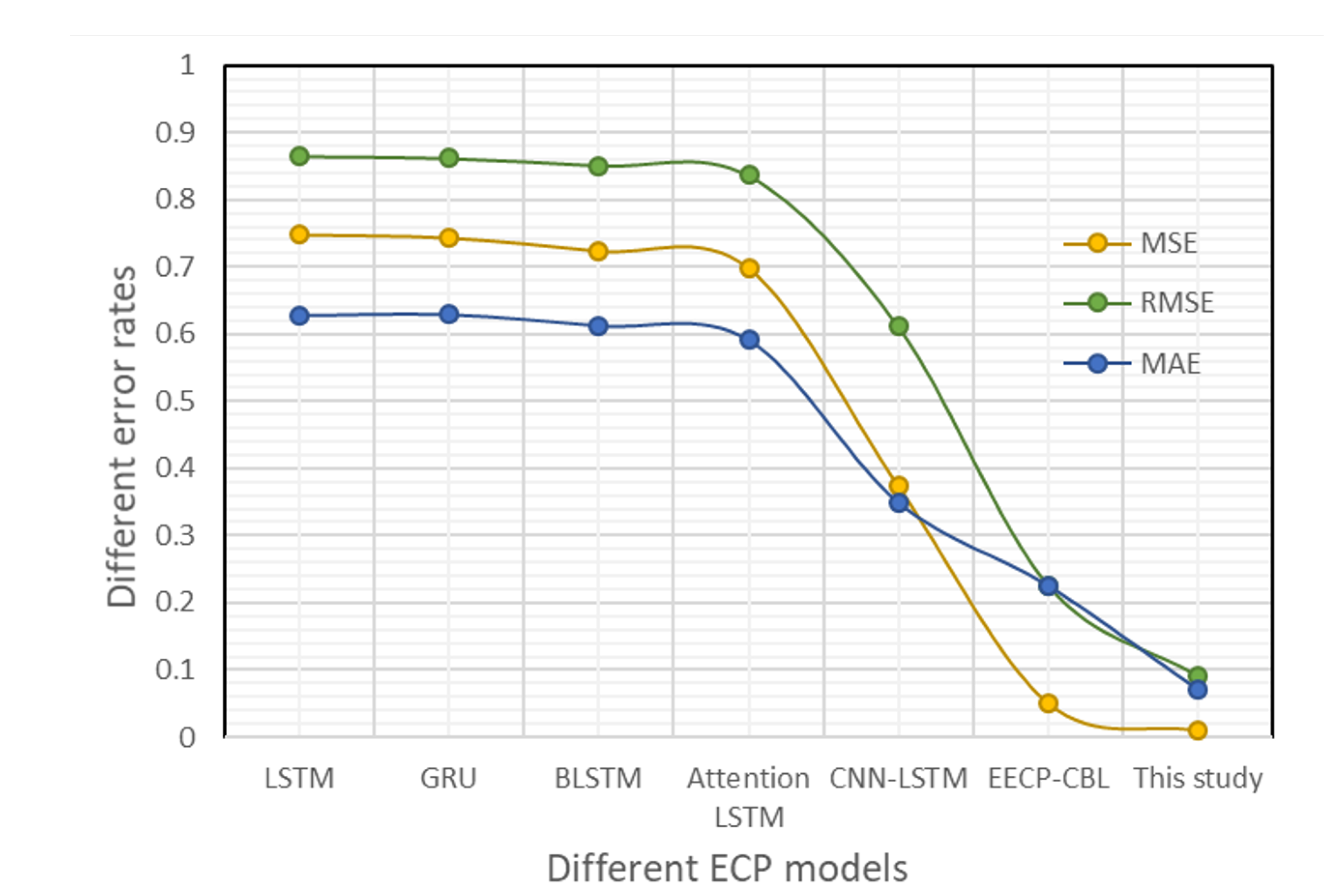
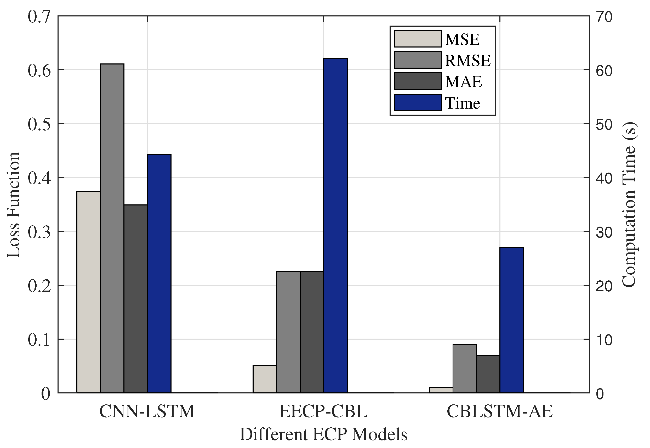
5.2. Comparison with State-of-the-Art

To verify the effectiveness of CBLSTM-AE for ECP, Figure 4 presents the comparison result of the proposed framework to other frameworks in the literature using the UCI dataset for daily ECP.

The proposed CBLSTM-AE achieved the lowest MSE, RMSE, and MAE compared to other frameworks, as illustrated in Figure 4. Specifically, the CBLSTM-AE achieved an MSE of $80\%$, RMSE of $60\%$, and MAE of $69\%$ performance increase to electric ECP-based CNN and BLSTM (EECP-CBL), and an MSE of $98.7\%$, RMSE of $89.6\%$, and MAE of $88.6\%$ performance increase to vanilla LSTM currently being used on the Q-Energy platform.

Comparing the computation time, including training and testing time shown in Figure 5, the proposed CBLSTM-AE achieves a $56\%$ performance increase to EECP-CBL, $38.8\%$ to CNN-LSTM, and a $75.2\%$ to vanilla LSTM. The reduction in computational time is particularly of interest because the algorithm will be deployed on IoT devices for the project.

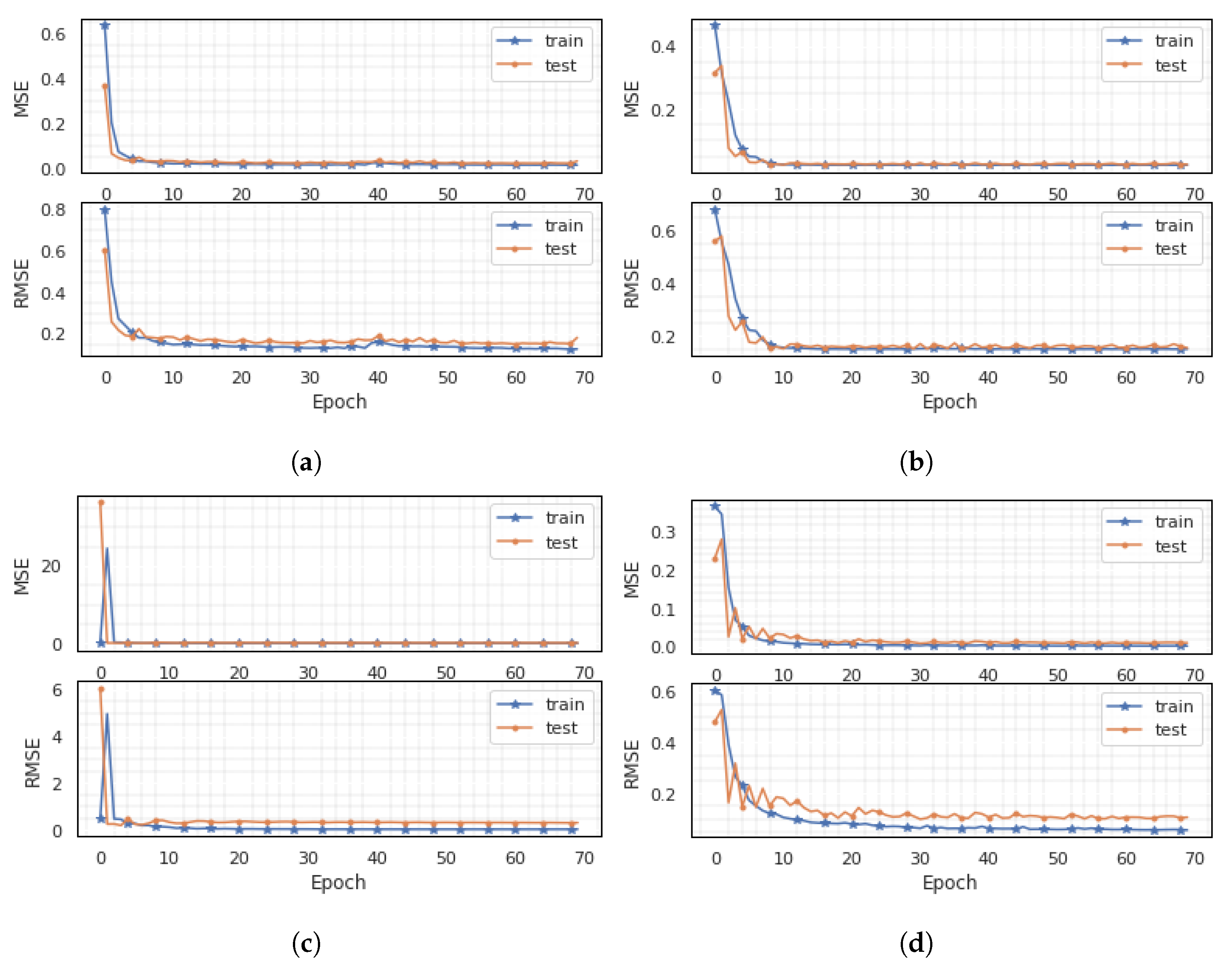
5.3. Generalisation Ability of CBLSTM-AE

Training a DNN that can generalise well to new data is a continuously challenging task due to the high volatility of the neurons [37]. A good generalisation to a different dataset is the ability to not underfit or overfit the learning data, or increase the optimisation time, thus leading to a better overall performance of the framework [37]. We used different Energy-IQ project datasets across Canada and the UK, described in Section 4.1, to evaluate the generalisation ability of the proposed framework. As the lengths of the datasets differ, for the datasets with more than a year and less than two years’ worth of data, we used the first year as the training set while the remaining months are used as the testing set. For a larger dataset, we used the previous years for training and the last year for testing.

The training and validation losses for the different datasets are shown in Figure 6. Figure 6a–d reflect the MSE and RMSE for the daily data for Hospital, Office, Restaurant, and Carehome, respectively. It can be observed from Figure 6 that the proposed predictive framework generalise well to new (not previously seen) problems with different physics. The recorded MSE is between $0.01$ and $0.17$ for all buildings, including the university with an average energy consumption profile of 9071 kWh for the campus under observation.

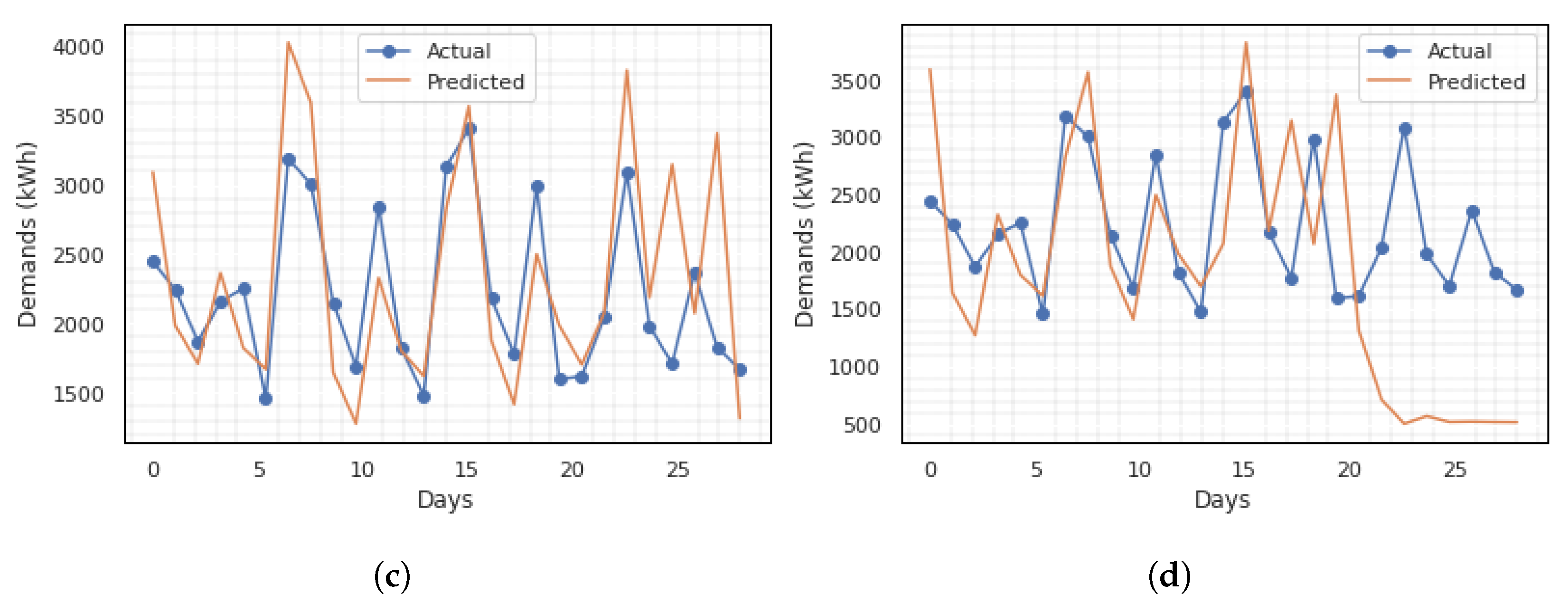
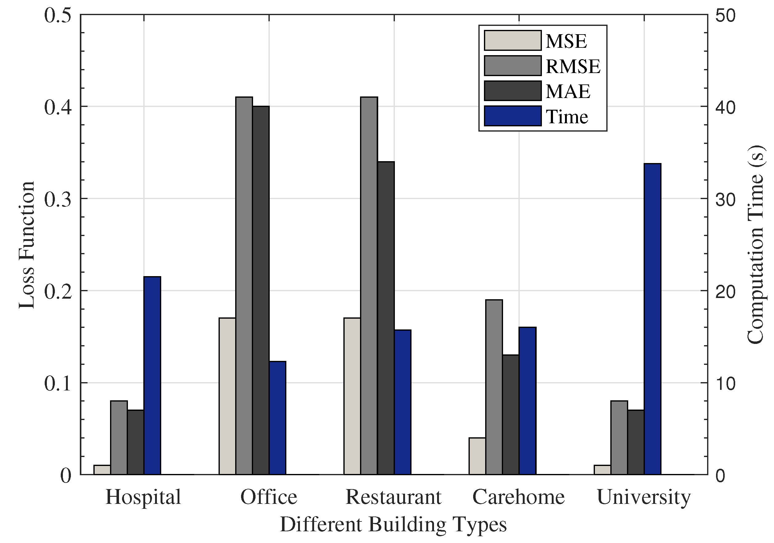
5.4. Performance Analysis for Different Dataset

To further ascertain the performance of CBLSTM-AE to several lengths of dataset, this section explores the different data more closely to give more insight into their impact on the predictive framework.

As expected, it can be observed from Figure 7 that the increase in the length of the dataset resulted in an increase in computation time. This is especially true for the length of data over 2 years, as seen with Hospital (144 weeks) and University (260 weeks). Interestingly, no linear relationship is observed between the computation time and data length for the data less than 2 years, as seen in the Office (12 s), Restaurant (15 s), and Carehome (17 s) datasets, with computation time lower than a lengthier dataset. Similarly, the longer the length of the dataset, as with the Hospital and the University, the lower the measured loss, signifying more accurate prediction ability of the predictive framework. Irrespective of the data length, the proposed CBLSTM-AE framework achieves a low MSE loss of 0.01–0.17 and computation time of 12–33 s for the varied datasets. However, while a short length of data resulted in low computation time and a little higher MSE loss, compared to other test results, a trade-off of accuracy and computation time exists in these test cases. As our focus for the project is both accuracy and computation time, on average, two years’ worth of data is appropriate to achieve the required aim.

6. Conclusions

This work proposed CBLSTM-AE, a hybrid deep learning framework to correctly predict the energy consumption of different building types that include commercial and domestics in Canada and the UK. The results show increased performance with a lower computation time of $56\%$ and $75.2\%$, and a mean squared error of $80\%$ and $98.7\%$, compared to EECP-CBL and vanilla LSTM, respectively. The results demonstrated a good generalisation with robustness against framework overfitting and underfitting, proving its predictive ability over varying datasets.

On the contrary, the limitation of this study is the extensive experimentation by trial and error in selecting the optimal hyperparameter values for the framework. We are working on a method to automate the selection of optimal hyperparameter values. In addition, in the UK and Canada scenario, it would have been interesting to compare the energy consumption situation due to their different environmental conditions that impact electricity predictions. This was not possible due to insufficient data to form a basis for comparison. In future work, we would compare the different situations as more data becomes available. Another identified future work is to extend the proposed framework for price forecast in an energy market, whilst analysing the impact of integrating renewable energy sources (solar, wind, and battery) on the energy demand and price forecast.

References

1. Velickov, S. Energy 4.0: Digital Twin for Electric Utilities, Grid Edge and Internet of Electricity. 2020. Available online: https://www.linkedin.com/pulse/energy-40-digital-twin-electric-utilities-grid-edge-slavco-velickov/ (accessed on 16 November 2020).
2. Bunn, D.; Farmer, E.D. Comparative Models for Electrical Load Forecasting; John Wiley and Sons Inc.: New York, NY, USA, 1985. [Google Scholar]
3. Chitalia, G.; Pipattanasomporn, M.; Garg, V.; Rahman, S. Robust short-term electrical load forecasting framework for commercial buildings using deep recurrent neural networks. Appl. Energy 2020, 278, 115410. [Google Scholar] [CrossRef]
4. Jogunola, O.; Adebisi, B.; Ikpehai, A.; Popoola, S.I.; Gui, G.; Gacanin, H.; Ci, S. Consensus Algorithms and Deep Reinforcement Learning in Energy Market: A Review. IEEE Internet Things J. 2020, 8, 4211–4227. [Google Scholar] [CrossRef]
5. Jogunola, O.; Wang, W.; Adebisi, B. Prosumers Matching and Least-Cost Energy Path Optimisation for Peer-to-Peer Energy Trading. IEEE Access 2020, 8, 95266–95277. [Google Scholar] [CrossRef]
6. Jogunola, O.; Tsado, Y.; Adebisi, B.; Hammoudeh, M. VirtElect: A Peer-to-Peer Trading Platform for Local Energy Transactions. IEEE Internet Things J. 2021. [Google Scholar] [CrossRef]
7. Kim, T.Y.; Cho, S.B. Predicting residential energy consumption using CNN-LSTM neural networks. Energy 2019, 182, 72–81. [Google Scholar] [CrossRef]
8. Khan, Z.A.; Hussain, T.; Ullah, A.; Rho, S.; Lee, M.; Baik, S.W. Towards Efficient Electricity Forecasting in Residential and Commercial Buildings: A Novel Hybrid CNN with a LSTM-AE based Framework. Sensors 2020, 20, 1399. [Google Scholar] [CrossRef] [Green Version]
9. Somu, N.; MR, G.R.; Ramamritham, K. A hybrid model for building energy consumption forecasting using long short term memory networks. Appl. Energy 2020, 261, 114131. [Google Scholar] [CrossRef]
10. Zaidi, B.H.; Ullah, I.; Alam, M.; Adebisi, B.; Azad, A.; Ansari, A.R.; Nawaz, R. Incentive Based Load Shedding Management in a Microgrid Using Combinatorial Auction with IoT Infrastructure. Sensors 2021, 21, 1935. [Google Scholar] [CrossRef]
11. Muzaffar, S.; Afshari, A. Short-term load forecasts using LSTM networks. Energy Procedia 2019, 158, 2922–2927. [Google Scholar] [CrossRef]
12. Dagdougui, H.; Bagheri, F.; Le, H.; Dessaint, L. Neural network model for short-term and very-short-term load forecasting in district buildings. Energy Build. 2019, 203, 109408. [Google Scholar] [CrossRef]
13. Fan, C.; Xiao, F.; Zhao, Y. A short-term building cooling load prediction method using deep learning algorithms. Appl. Energy 2017, 195, 222–233. [Google Scholar] [CrossRef]
14. Kim, J.; Moon, J.; Hwang, E.; Kang, P. Recurrent inception convolution neural network for multi short-term load forecasting. Energy Build. 2019, 194, 328–341. [Google Scholar] [CrossRef]
15. Cai, M.; Pipattanasomporn, M.; Rahman, S. Day-ahead building-level load forecasts using deep learning vs. traditional time-series techniques. Appl. Energy 2019, 236, 1078–1088. [Google Scholar] [CrossRef]
16. Wang, Z.; Wang, Y.; Zeng, R.; Srinivasan, R.S.; Ahrentzen, S. Random Forest based hourly building energy prediction. Energy Build. 2018, 171, 11–25. [Google Scholar] [CrossRef]
17. Candanedo, L.M.; Feldheim, V.; Deramaix, D. Data driven prediction models of energy use of appliances in a low-energy house. Energy Build. 2017, 140, 81–97. [Google Scholar] [CrossRef]
18. Le, T.; Vo, M.T.; Vo, B.; Hwang, E.; Rho, S.; Baik, S.W. Improving electric energy consumption prediction using CNN and Bi-LSTM. Appl. Sci. 2019, 9, 4237. [Google Scholar] [CrossRef] [Green Version]
19. Ullah, F.U.M.; Ullah, A.; Haq, I.U.; Rho, S.; Baik, S.W. Short-term prediction of residential power energy consumption via CNN and multi-layer bi-directional LSTM networks. IEEE Access 2019, 8, 123369–123380. [Google Scholar] [CrossRef]
20. Massana, J.; Pous, C.; Burgas, L.; Melendez, J.; Colomer, J. Short-term load forecasting in a non-residential building contrasting models and attributes. Energy Build. 2015, 92, 322–330. [Google Scholar] [CrossRef] [Green Version]
21. Yildiz, B.; Bilbao, J.I.; Sproul, A.B. A review and analysis of regression and machine learning models on commercial building electricity load forecasting. Renew. Sustain. Energy Rev. 2017, 73, 1104–1122. [Google Scholar] [CrossRef]
22. Walter, T.; Price, P.N.; Sohn, M.D. Uncertainty estimation improves energy measurement and verification procedures. Appl. Energy 2014, 130, 230–236. [Google Scholar] [CrossRef] [Green Version]
23. Gianniou, P.; Liu, X.; Heller, A.; Nielsen, P.S.; Rode, C. Clustering-based analysis for residential district heating data. Energy Convers. Manag. 2018, 165, 840–850. [Google Scholar] [CrossRef]
24. Khan, A.; Chiroma, H.; Imran, M.; Bangash, J.I.; Asim, M.; Hamza, M.F.; Aljuaid, H. Forecasting electricity consumption based on machine learning to improve performance: A case study for the organization of petroleum exporting countries (OPEC). Comput. Electr. Eng. 2020, 86, 106737. [Google Scholar] [CrossRef]
25. Zhong, H.; Wang, J.; Jia, H.; Mu, Y.; Lv, S. Vector field-based support vector regression for building energy consumption prediction. Appl. Energy 2019, 242, 403–414. [Google Scholar] [CrossRef]
26. Ahmad, M. Seasonal decomposition of electricity consumption data. Rev. Integr. Bus. Econ. Res. 2017, 6, 271. [Google Scholar]
27. Fayaz, M.; Shah, H.; Aseere, A.M.; Mashwani, W.K.; Shah, A.S. A framework for prediction of household energy consumption using feed forward back propagation neural network. Technologies 2019, 7, 30. [Google Scholar] [CrossRef] [Green Version]
28. Fayaz, M.; Kim, D. A prediction methodology of energy consumption based on deep extreme learning machine and comparative analysis in residential buildings. Electronics 2018, 7, 222. [Google Scholar] [CrossRef]
29. Li, C.; Ding, Z.; Zhao, D.; Yi, J.; Zhang, G. Building energy consumption prediction: An extreme deep learning approach. Energies 2017, 10, 1525. [Google Scholar] [CrossRef]
30. Almalaq, A.; Zhang, J.J. Evolutionary deep learning-based energy consumption prediction for buildings. IEEE Access 2018, 7, 1520–1531. [Google Scholar] [CrossRef]
31. Wen, L.; Zhou, K.; Yang, S.; Lu, X. Optimal load dispatch of community microgrid with deep learning based solar power and load forecasting. Energy 2019, 171, 1053–1065. [Google Scholar] [CrossRef]
32. Hebrail, G.; Berard, A. Individual Household Electric Power Consumption Data Set. Available online: https://archive.ics.uci.edu/ml/datasets/individual+household+electric+power+consumption (accessed on 16 November 2020).
33. Shi, H.; Xu, M.; Li, R. Deep learning for household load forecasting—A novel pooling deep RNN. IEEE Trans. Smart Grid 2017, 9, 5271–5280. [Google Scholar] [CrossRef]
34. Ullah, A.; Haydarov, K.; Ul Haq, I.; Muhammad, K.; Rho, S.; Lee, M.; Baik, S.W. Deep learning assisted buildings energy consumption profiling using smart meter data. Sensors 2020, 20, 873. [Google Scholar] [CrossRef] [PubMed] [Green Version]
35. Ullah, I.; Ahmad, R.; Kim, D. A prediction mechanism of energy consumption in residential buildings using hidden markov model. Energies 2018, 11, 358. [Google Scholar] [CrossRef] [Green Version]
36. Google. Welcome to Colaboratory. 2020. Available online: https://colab.research.google.com/ (accessed on 16 November 2020).
37. Brownlee, J. Better Deep Learning: Train Faster, Reduce Overfitting, and Make Better Predictions; Machine Learning Mastery: Melbourne, Australia, 2018. [Google Scholar]
Figure 1. Proposed CBLSTM-AE energy prediction framework.
Energies 15 00810 g001
Figure 2. The 28 days actual vs. predicted value for different input sizes. (a) 7 days input; (b) 14 days input; (c) 21 days input; (d) 28 days input.
Energies 15 00810 g002aEnergies 15 00810 g002b
Figure 3. Training and validation loss during training.
Energies 15 00810 g003
Figure 4. Performance comparison to other frameworks for daily data.
Energies 15 00810 g004
Figure 5. Performance comparison to other frameworks with computation time.
Energies 15 00810 g005
Figure 6. Training and validation loss during training for different daily datasets for generalisation performance. (a) Hospital; (b) Office; (c) Restaurant; (d) Carehome.
Energies 15 00810 g006
Figure 7. Comparison result of different energy consumption dataset.
Energies 15 00810 g007