
Extended Rauch–Tung–Striebel Smoother for the State of Charge Estimation of Lithium-Ion Batteries Based on an Enhanced Circuit Model

Abstract
:1. Introduction
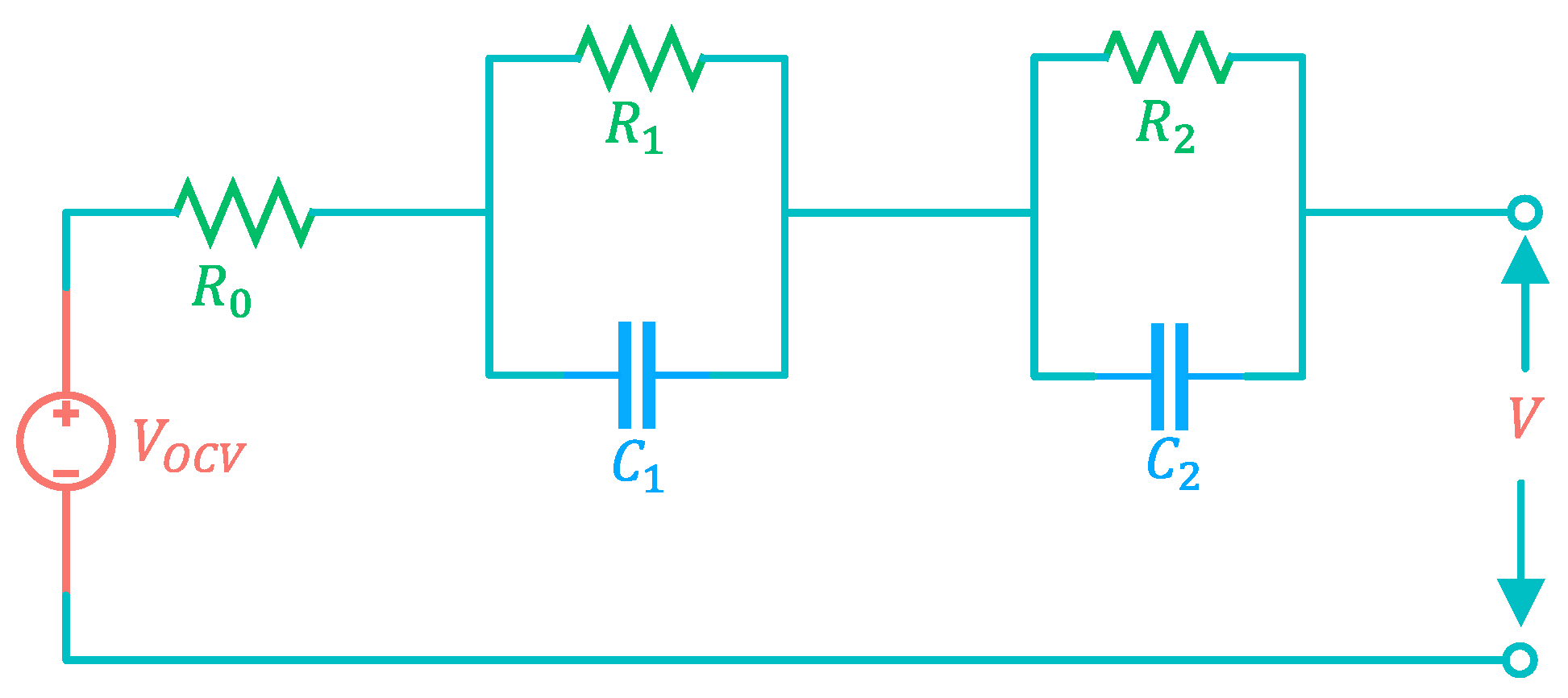
2. Enhanced Equivalent Circuit Model of Lithium-Ion Battery
2.1. Fundamental Equivalent Circuit Model
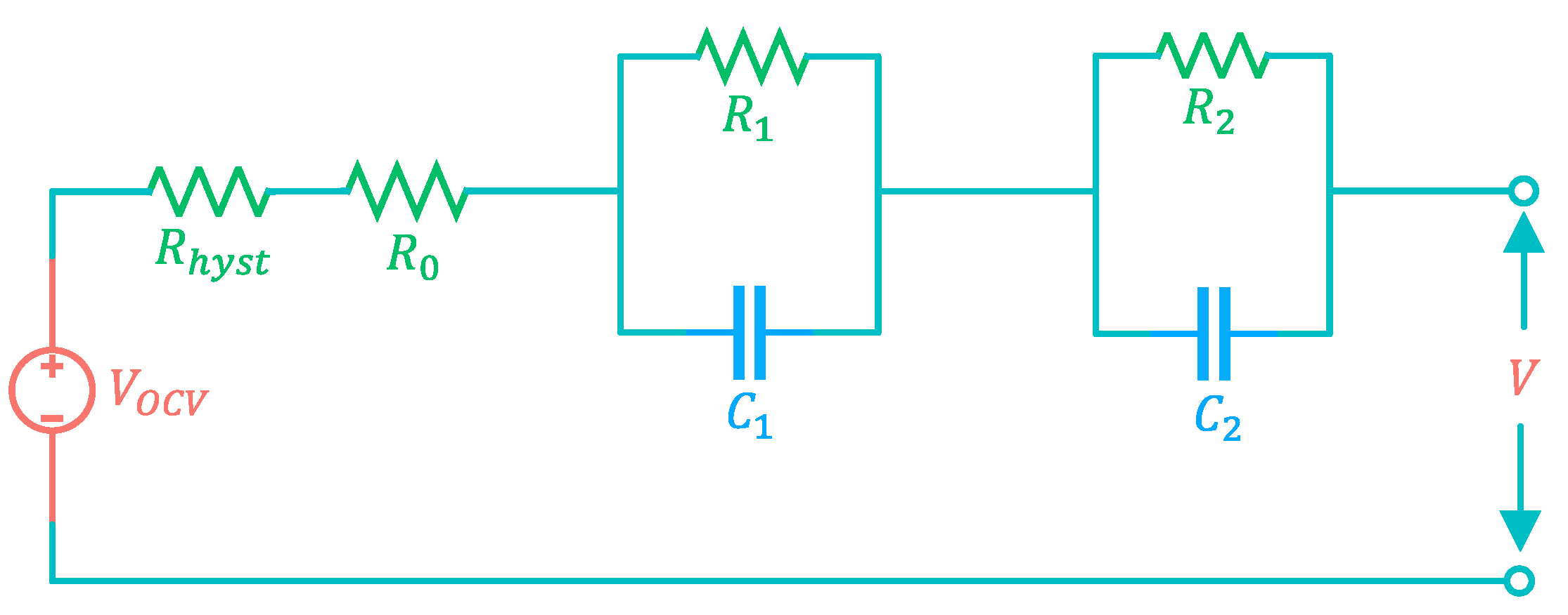
2.2. Hysteresis Voltage
2.3. Enhanced Circuit Model
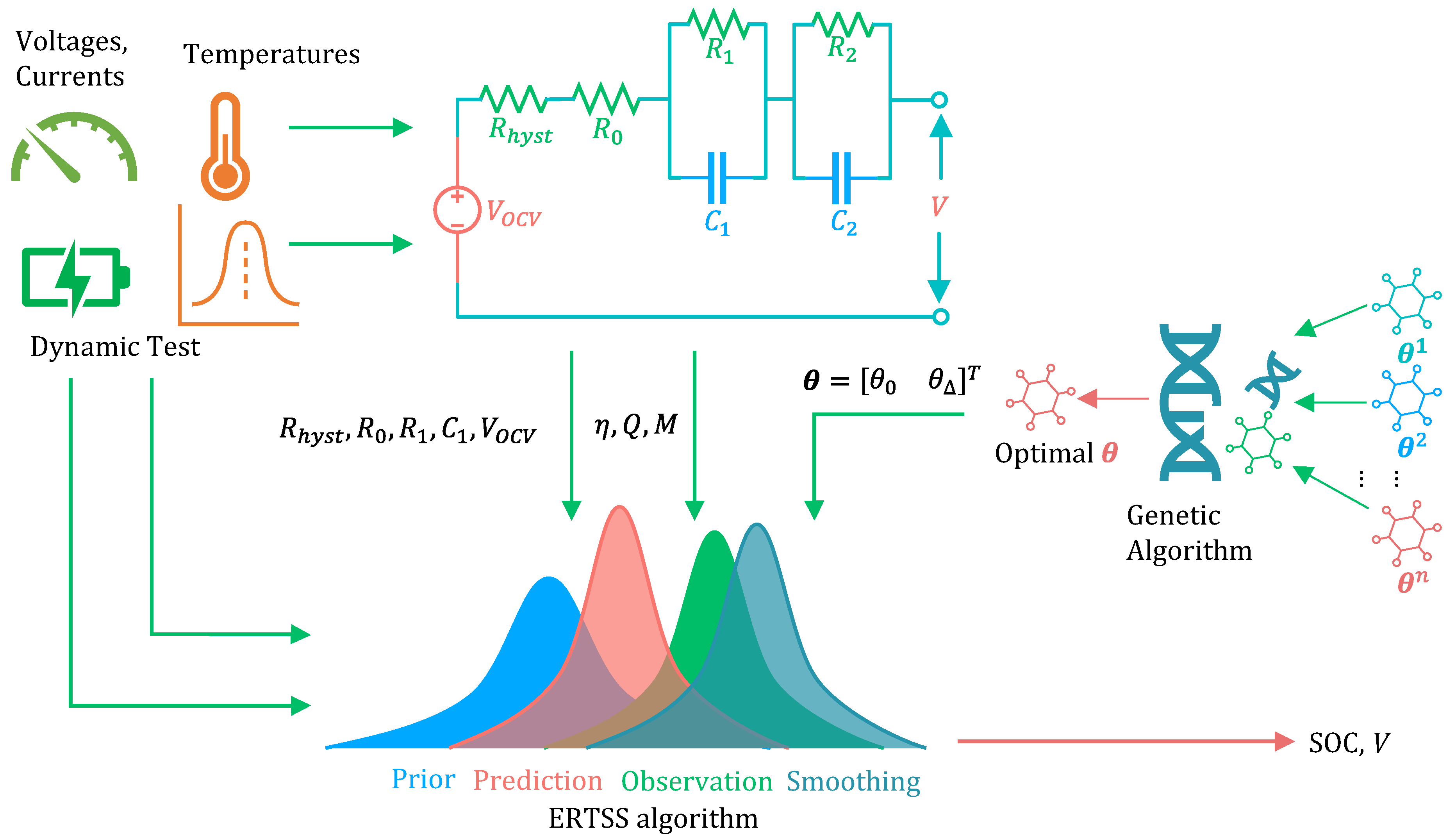
3. SOC Estimation
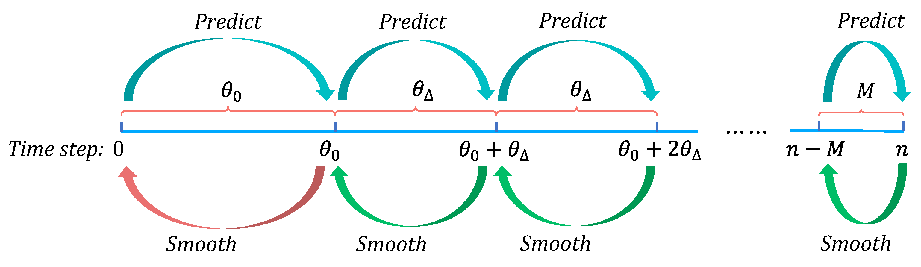
3.1. ERTSS
3.2. Genetic Algorithm
4. Experiment and Validation
4.1. Battery Test
4.2. Cell Model Parameters Identification
- Extract the OCV and Q parameters from the OCV test data.
- Apply the dynamic tests’ current data to calculate the and parameters with a given initial.
- Use a subspace identification method to obtain , , , parameters.
- Transform Equation (19) into a vectorize equation:Then obtain X parameters through the least-squares equation .
- Apply optimization algorithm to obtain with a cost function:where m denotes the size of the test data, is the estimation cell voltage with a given , and v is the measured cell voltage during the test.
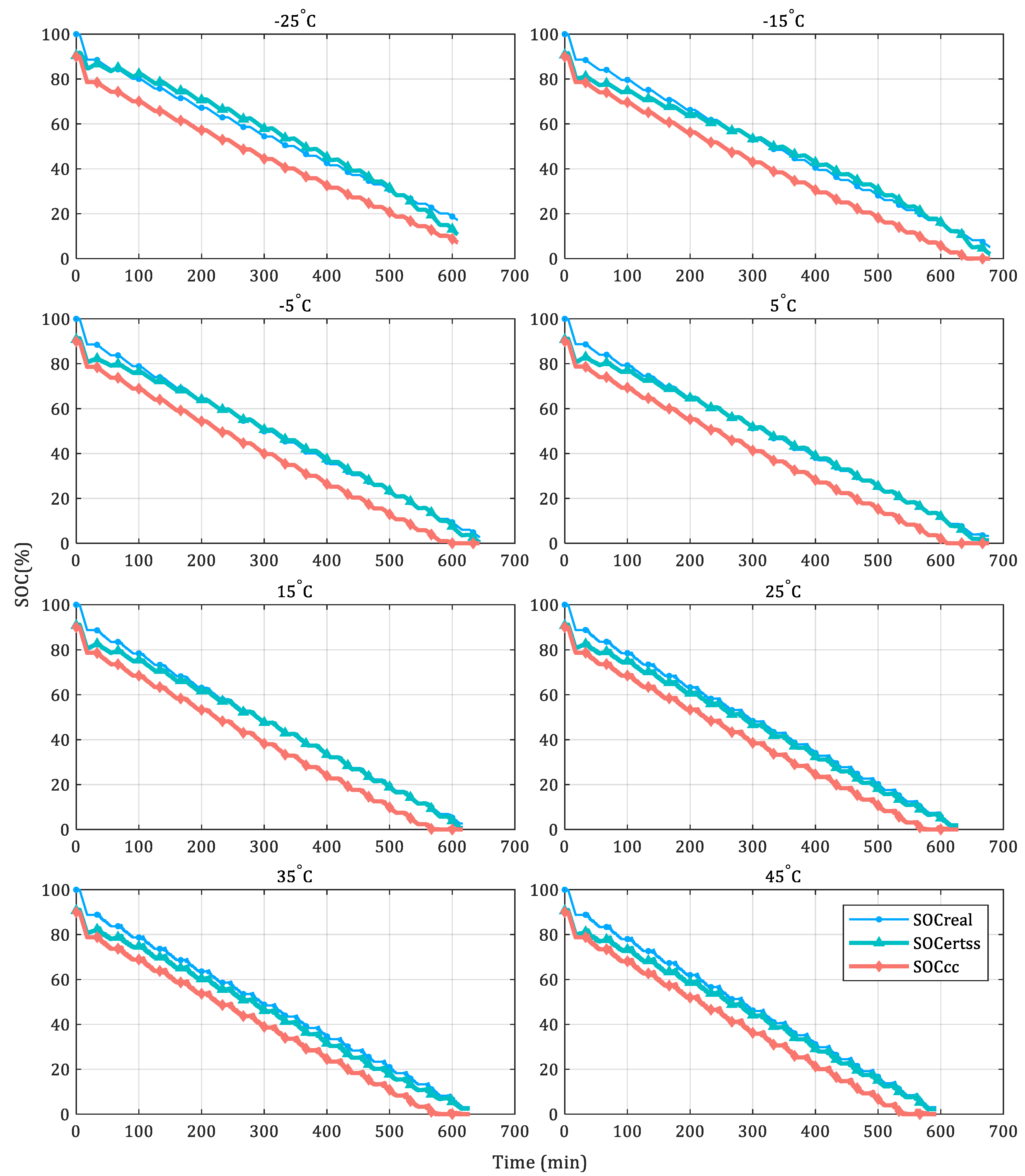
4.3. ERTSS Estimation
- As it uses all measurements over a time interval, the smoothing step can be used as an interpolation when some measurements are missing or abnormal, such as the safety mode of some battery systems when the current sensor has an open-wire fault.
- For the energy networks with battery storage systems, which may not require strict real-time estimation, the ERTSS could optimize the SOC estimations before the current time step. These will help the further power supply.
- Since the smoothing step decreases the estimation error, it will help to improve the optimization of power flow in hybrid electric vehicles.
- The state transformation matrix can be computed offline and saved as a lookup table, whereas the cell capacity Q and ohmic resistance should be updated by the state of health estimations.
- The smoothing step of ERTSS needs more storage space than the EKF for saving the measurements and estimations at every time interval. If there are serious storage limitations, a small time interval should be chosen.
- The SOC changes quickly for some applications, such as an A0 class electric vehicle with a small battery. ERTSS requires more computation than EKF, the smoothing step time must be evaluated if it sacrifices the SOC refresh rate.
5. Conclusions
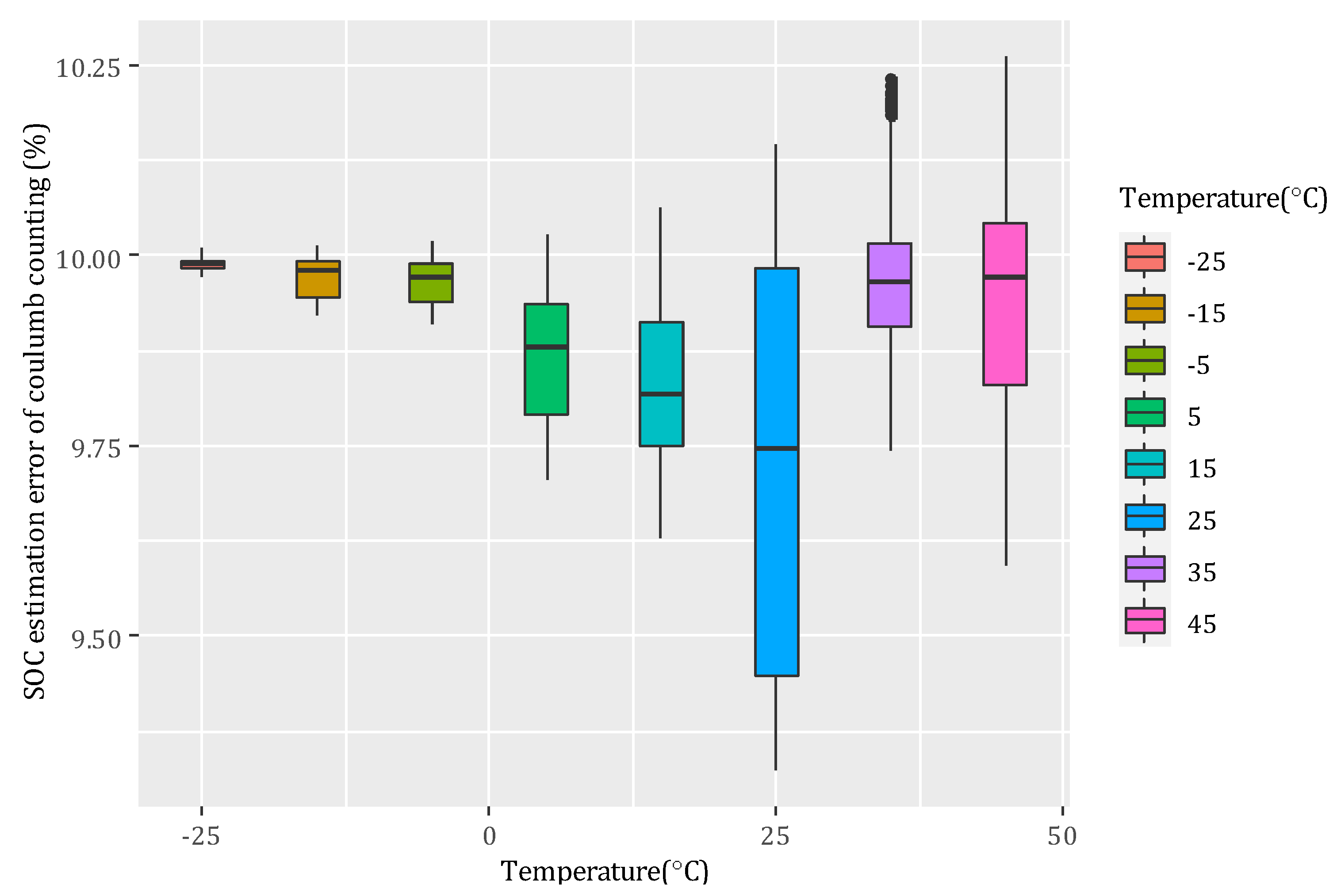
- The ERTSS method can estimate SOC with an accuracy of approximately 4% as the ambient temperature changes from −25 C to 45 C with an initial error of 10%. In low-temperature and high-temperature applications, the ERTSS accuracy decreases, but it is still better than the CC and the EKF.
- The ERTSS method is a bit more complicated than the EKF method. There is only one more prediction step than for the EKF, so it is acceptable to consider improvements in estimation accuracy and more minor deviations for many safety-critical applications.
Author Contributions
Funding
Institutional Review Board Statement
Informed Consent Statement
Data Availability Statement
Conflicts of Interest
Abbreviations
| APF | Adaptive Particle Filter |
| BMS | Battery Management System |
| CC | Coulomb Counting |
| EKF | Extended Kalman Filter |
| ERTSS | Extended Rauch–Tung–Striebel Smoother |
| GA | Genetic Algorithm |
| LFP | Lithium Iron Phosphate |
| OCV | Open Circuit Voltage |
| RC | Resistance-Capacitance |
| RTS | Rauch–Tung–Striebel |
| RTSS | Rauch–Tung–Striebel Smoother |
| SOC | State of Charge |
| SOH | State of Health |
| UKF | Unscented Particle Filter |
References
- Park, S.; Jeong, S.Y.; Lee, T.K.; Park, M.W.; Lim, H.Y.; Sung, J.; Cho, J.; Kwak, S.K.; Hong, S.Y.; Choi, N.S. Replacing conventional battery electrolyte additives with dioxolone derivatives for high-energy-density lithium-ion batteries. Nat. Commun. 2021, 12, 1–12. [Google Scholar] [CrossRef] [PubMed]
- Armand, M.; Axmann, P.; Bresser, D.; Copley, M.; Edström, K.; Ekberg, C.; Guyomard, D.; Lestriez, B.; Novák, P.; Petranikova, M.; et al. Lithium-ion batteries–Current state of the art and anticipated developments. J. Power Sources 2020, 479, 228708. [Google Scholar] [CrossRef]
- Yu, Q.; Wan, C.; Li, J.; Zhang, X.; Huang, Y.; Liu, T. An Open Circuit Voltage Model Fusion Method for State of Charge Estimation of Lithium-Ion Batteries. Energies 2021, 14, 1797. [Google Scholar] [CrossRef]
- Knap, V.; Stroe, D.I. Effects of open-circuit voltage tests and models on state-of-charge estimation for batteries in highly variable temperature environments: Study case nano-satellites. J. Power Sources 2021, 498, 229913. [Google Scholar] [CrossRef]
- Meng, J.; Ricco, M.; Acharya, A.B.; Luo, G.; Swierczynski, M.; Stroe, D.I.; Teodorescu, R. Low-complexity online estimation for LiFePO4 battery state of charge in electric vehicles. J. Power Sources 2018, 395, 280–288. [Google Scholar] [CrossRef]
- Ren, Z.; Du, C.; Wu, Z.; Shao, J.; Deng, W. A comparative study of the influence of different open circuit voltage tests on model-based state of charge estimation for lithium-ion batteries. Int. J. Energy Res. 2021, 45, 13692–13711. [Google Scholar] [CrossRef]
- Espedal, I.B.; Jinasena, A.; Burheim, O.S.; Lamb, J.J. Current Trends for State-of-Charge (SoC) Estimation in Lithium-Ion Battery Electric Vehicles. Energies 2021, 14, 3284. [Google Scholar] [CrossRef]
- Su, L.; Zhou, G.; Hu, D.; Liu, Y.; Zhu, Y. Research on the State of Charge of Lithium-Ion Battery Based on the Fractional Order Model. Energies 2021, 14, 6307. [Google Scholar] [CrossRef]
- Wu, L.; Liu, K.; Pang, H.; Jin, J. Online SOC Estimation Based on Simplified Electrochemical Model for Lithium-Ion Batteries Considering Current Bias. Energies 2021, 14, 5265. [Google Scholar] [CrossRef]
- Rzepka, B.; Bischof, S.; Blank, T. Implementing an Extended Kalman Filter for SoC Estimation of a Li-Ion Battery with Hysteresis: A Step-by-Step Guide. Energies 2021, 14, 3733. [Google Scholar] [CrossRef]
- Li, W.; Fan, Y.; Ringbeck, F.; Jöst, D.; Han, X.; Ouyang, M.; Sauer, D.U. Electrochemical model-based state estimation for lithium-ion batteries with adaptive unscented Kalman filter. J. Power Sources 2020, 476, 228534. [Google Scholar] [CrossRef]
- Li, W.; Zhang, J.; Ringbeck, F.; Jöst, D.; Zhang, L.; Wei, Z.; Sauer, D.U. Physics-informed neural networks for electrode-level state estimation in lithium-ion batteries. J. Power Sources 2021, 506, 230034. [Google Scholar] [CrossRef]
- Ringbeck, F.; Garbade, M.; Sauer, D.U. Uncertainty-aware state estimation for electrochemical model-based fast charging control of lithium-ion batteries. J. Power Sources 2020, 470, 228221. [Google Scholar] [CrossRef]
- Hasan, R.; Scott, J. Extending Randles’s Battery Model to Predict Impedance, Charge–Voltage, and Runtime Characteristics. IEEE Access 2020, 8, 85321–85328. [Google Scholar] [CrossRef]
- Wei, Z.; Zou, C.; Leng, F.; Soong, B.H.; Tseng, K.J. Online Model Identification and State-of-Charge Estimate for Lithium-Ion Battery With a Recursive Total Least Squares-Based Observer. IEEE Trans. Ind. Electron. 2018, 65, 1336–1346. [Google Scholar] [CrossRef]
- He, J.; Wei, Z.; Bian, X.; Yan, F. State-of-Health Estimation of Lithium-Ion Batteries Using Incremental Capacity Analysis Based on Voltage-Capacity Model. IEEE Trans. Transp. Electrif. 2020, 6, 417–426. [Google Scholar] [CrossRef]
- Lee, J.H.; Lee, I.S. Lithium Battery SOH Monitoring and an SOC Estimation Algorithm Based on the SOH Result. Energies 2021, 14, 4506. [Google Scholar] [CrossRef]
- Yan, G.; Liu, D.; Li, J.; Mu, G. A cost accounting method of the Li-ion battery energy storage system for frequency regulation considering the effect of life degradation. Prot. Control Mod. Power Syst. 2018, 3, 1–9. [Google Scholar] [CrossRef]
- Wei, Z.; Zhao, J.; Xiong, R.; Dong, G.; Pou, J.; Tseng, K.J. Online Estimation of Power Capacity With Noise Effect Attenuation for Lithium-Ion Battery. IEEE Trans. Ind. Electron. 2019, 66, 5724–5735. [Google Scholar] [CrossRef]
- Zhu, Q.; Li, L.; Hu, X.; Xiong, N.; Hu, G.D. H∞-Based Nonlinear Observer Design for State of Charge Estimation of Lithium-Ion Battery With Polynomial Parameters. IEEE Trans. Veh. Technol. 2017, 66, 10853–10865. [Google Scholar] [CrossRef]
- Hannan, M.A.; Lipu, M.H.; Hussain, A.; Mohamed, A. A review of lithium-ion battery state of charge estimation and management system in electric vehicle applications: Challenges and recommendations. Renew. Sustain. Energy Rev. 2017, 78, 834–854. [Google Scholar] [CrossRef]
- Li, J.; Gao, F.; Yan, G.; Zhang, T.; Li, J. Modeling and SOC estimation of lithium iron phosphate battery considering capacity loss. Prot. Control Mod. Power Syst. 2018, 3, 1–9. [Google Scholar] [CrossRef] [Green Version]
- Li, L.; Wang, C.; Yan, S.; Zhao, W. A combination state of charge estimation method for ternary polymer lithium battery considering temperature influence. J. Power Sources 2021, 484, 229204. [Google Scholar] [CrossRef]
- Wei, Z.; Dong, G.; Zhang, X.; Pou, J.; Quan, Z.; He, H. Noise-immune model identification and state-of-charge estimation for lithium-ion battery using bilinear parameterization. IEEE Trans. Ind. Electron. 2020, 68, 312–323. [Google Scholar] [CrossRef]
- Shu, X.; Li, G.; Shen, J.; Yan, W.; Chen, Z.; Liu, Y. An adaptive fusion estimation algorithm for state of charge of lithium-ion batteries considering wide operating temperature and degradation. J. Power Sources 2020, 462, 228132. [Google Scholar] [CrossRef]
- Qiu, X.; Wu, W.; Wang, S. Remaining useful life prediction of lithium-ion battery based on improved cuckoo search particle filter and a novel state of charge estimation method. J. Power Sources 2020, 450, 227700. [Google Scholar] [CrossRef]
- Mawonou, K.S.; Eddahech, A.; Dumur, D.; Beauvois, D.; Godoy, E. Improved state of charge estimation for Li-ion batteries using fractional order extended Kalman filter. J. Power Sources 2019, 435, 226710. [Google Scholar] [CrossRef]
- Zhou, Z.; Duan, B.; Kang, Y.; Cui, N.; Shang, Y.; Zhang, C. A low-complexity state of charge estimation method for series-connected lithium-ion battery pack used in electric vehicles. J. Power Sources 2019, 441, 226972. [Google Scholar] [CrossRef]
- Zhang, W.; Wang, L.; Wang, L.; Liao, C. An improved adaptive estimator for state-of-charge estimation of lithium-ion batteries. J. Power Sources 2018, 402, 422–433. [Google Scholar] [CrossRef]
- Särkkä, S. Bayesian Filtering and Smoothing; Cambridge University Press: Cambridge, UK, 2013. [Google Scholar]
- Grewal, M.S.; Andrews, A.P. Kalman Filtering: Theory and Practice with Matlab; John Wiley & Sons: Hoboken, NJ, USA, 2014. [Google Scholar]
- Plett, G.L. Battery Management Systems, Volume I: Battery Modeling; Artech House: London, UK, 2015. [Google Scholar]
- Plett, G.L. Battery Management Systems, Volume II: Equivalent-Circuit Methods; Artech House: London, UK, 2016. [Google Scholar]
- Idaho National Engineering Laboratory, EG & G Idaho. A Simplified Version of the Federal Urban Driving Schedule for Electric Vehicle Battery Testing; US Department of Energy Report DOE/ID-10146; US Department of Energy: Washington, DC, USA, 1988. [Google Scholar]


| Authors | Methods | Model | Error |
|---|---|---|---|
| Knap V. et al. [4] | unscented Kalman filter (UKF) | an open circuit voltage (OCV) model | Mean RMSE: <=4.2% (@5 C–45 C) |
| Li L. et al. [23] | Adaptive particle filter and coulomb counting | a temperature correction equivalent circuit model | Maximum absolute error <=3.64% (@−5 C–15 C) |
| Wei Z. et al. [24] | a Luenberger observer | first-order RC model | RMSE: <=0.89% (@22 C) |
| Xing Shu [25] | adaptive H-infinity filter | first-order RC model | Maximum absolute error <=0.7% (@25 C) |
| Li W. et al. [11] | adaptive unscented Kalman filter (UKF) | reduced-order electrochemical models | Mean absolute error: <=2.81% (@25 C) |
| Qiu X. et al. [26] | multiscale hybrid Kalman filter (MHKF) | second-order RC model | Maximum absolute error: <=1.41% (@25 C) |
| Mawonou K. et al. [27] | extended Kalman filter (EKF) | a fractional order model (FOM) | Maximum absolute error: <=6.58% (@0 C) |
| Zhou Z. et al. [28] | recursive least squares-adaptive EKF | first-order RC model | Maximum absolute error: <=1.6% (@25 C) |
| Zhang W. et al. [29] | adaptive UKF | first-order RC model | Root mean square error: <=1.56% (@25 C) |
| Parameters | Value |
|---|---|
| Nominal capacity | 6 Ah at 25 C |
| Discharge cutoff voltage | 2.0 V |
| Charge cutoff voltage | 4.2 V |
| Nominal open circuit voltage | 3.6 V |
| Parameters | −25 C | −15 C | −5 C | 5 C | 15 C | 25 C | 35 C | 45 C |
|---|---|---|---|---|---|---|---|---|
| 0.9830 | 0.9844 | 0.9833 | 0.9883 | 0.9894 | 0.9929 | 0.9942 | 0.9953 | |
| Q | 5.0755 | 5.0791 | 5.0656 | 5.1331 | 5.1044 | 5.1344 | 5.1629 | 5.1432 |
| 65.7728 | 5.4554 | 250.00 | 103.048 | 58.1570 | 61.7498 | 59.0179 | 1.0000 | |
| 0.0167 | 0.0199 | 0.0091 | 0 | 0.0003 | 0.0025 | 0.0035 | 0.0026 | |
| M | 0.2362 | 0.1558 | 0.0852 | 0.0809 | 0.0614 | 0.0443 | 0.0336 | 0.0971 |
| 0.2151 | 0.1280 | 0.0661 | 0.0312 | 0.0179 | 0.0112 | 0.0081 | 0.0058 | |
| 0.8887 | 0.9571 | 1.2866 | 1.8302 | 2.4261 | 2.4107 | 2.5699 | 2.7953 | |
| 0.0984 | 0.0484 | 0.0202 | 0.0072 | 0.0052 | 0.0025 | 0.0020 | 0.0022 |
Publisher’s Note: MDPI stays neutral with regard to jurisdictional claims in published maps and institutional affiliations. |
© 2022 by the authors. Licensee MDPI, Basel, Switzerland. This article is an open access article distributed under the terms and conditions of the Creative Commons Attribution (CC BY) license (https://creativecommons.org/licenses/by/4.0/).
Share and Cite
Jiang, Y.; Song, W.; Zhu, H.; Zhu, Y.; Du, Y.; Yin, H. Extended Rauch–Tung–Striebel Smoother for the State of Charge Estimation of Lithium-Ion Batteries Based on an Enhanced Circuit Model. Energies 2022, 15, 963. https://doi.org/10.3390/en15030963
Jiang Y, Song W, Zhu H, Zhu Y, Du Y, Yin H. Extended Rauch–Tung–Striebel Smoother for the State of Charge Estimation of Lithium-Ion Batteries Based on an Enhanced Circuit Model. Energies. 2022; 15(3):963. https://doi.org/10.3390/en15030963
Chicago/Turabian StyleJiang, Yinfeng, Wenxiang Song, Hao Zhu, Yun Zhu, Yongzhi Du, and Huichun Yin. 2022. "Extended Rauch–Tung–Striebel Smoother for the State of Charge Estimation of Lithium-Ion Batteries Based on an Enhanced Circuit Model" Energies 15, no. 3: 963. https://doi.org/10.3390/en15030963
APA StyleJiang, Y., Song, W., Zhu, H., Zhu, Y., Du, Y., & Yin, H. (2022). Extended Rauch–Tung–Striebel Smoother for the State of Charge Estimation of Lithium-Ion Batteries Based on an Enhanced Circuit Model. Energies, 15(3), 963. https://doi.org/10.3390/en15030963