Permanent Magnet Synchronous Motor Model Extension for High-Frequency Signal Injection-Based Sensorless Magnet Polarity Detection

Abstract

In this paper, a novel extended permanent magnet synchronous motor model is presented that incorporates a quadratic flux-current function to represent the polarity-dependent saliency. The proposed model enables the design of sensorless polarity detection algorithms required by the initial position detection of permanent magnet synchronous motors. The novelty of the model is that it integrates the polarity-dependent saliency into the traditional machine model and introduces a new machine parameter, the polarity-dependent saliency coefficient, to specify the Hessian matrix of the flux-current function. A measurement method is presented for determination of the elements of the Hessian and the polarity-dependent saliency coefficient. The solution of the model is given for high-frequency sinusoidal pulsating voltage injection. Experimental results show that the proposed extended model accurately predicts the amplitudes and phases of the second harmonics of the motor currents, which are the carriers of the polarity-dependent information. This information enables a current measurement-based polarity detection algorithm using the phase difference between the fundamental and second harmonic of the apparent d-axis current. Both the presented measurement data and the proposed model show that injection in the d-direction is optimal for polarity detection.

1. Introduction

To meet the industrial performance and efficiency requirements, synchronous machines have been adopted in a wide variety of applications ranging from household appliances to industrial robots, electric vehicles and wind power systems [1,2,3]. Permanent magnet synchronous motors (PMSMs) are attractive candidates for high-performance, high-precision and highly dynamic engineering applications because of their high power density, high efficiency and high torque-to-volume ratio [4,5]. The field-oriented control of the PMSM drive requires phase current and rotor position feedback. To start the motor without mechanical alignment, reverse rotation and unwanted oscillations, it is also necessary to determine the initial rotor position including magnet polarity [6].

The operation of a traditional PMSM drive requires a shaft-mounted optical encoder or a resolver to determine the rotor position. However, in many industrial installations, the application of the shaft sensor increases the cost and size of the motor, reduces the reliability and the overall ruggedness of the drive, and limits the application in harsh environments [5,7,8]. Furthermore, many shaft sensors provide the initial rotor position with an inadequate resolution and incremental encoders do not provide it at all. Position-sensorless control schemes allow the elimination of shaft-mounted sensors as well as related electronics and wiring resulting in a more robust and cost-effective PMSM drive system. In addition, employing sensorless algorithms and shaft sensors simultaneously can increase reliability by introducing redundancy in safety critical applications [9,10].

1.1. Sensorless Control Methods for PMSMs

Position-sensorless control methods for PMSMs determine the rotor position in terms of electrical angle without a mechanical shaft sensor usually based on phase current measurements and a suitable machine model. Sensorless control techniques that rely on the fundamental excitation model are capable of providing high-performance control above about 3% of the nominal speed when the back electromotive force (back-EMF) is sufficiently large [11,12,13,14,15]. To extend the sensorless operation range towards zero speed, saliency-based methods have been proposed that rely on inductance variation due to geometrical and saturation effects [16,17]. These techniques exploit the anisotropic properties of PM machines, caused by the saliency of an interior permanent magnet rotor and/or the saturation of the stator and rotor iron cores.

The operation of anisotropy tracking techniques is either based on fundamental pulse-width modulation (PWM) excitation or signal injection. Modulated sinusoidal high-frequency signal injection (HFSI) methods primarily inject a high-frequency carrier signal with a small amplitude using either a rotating space vector in the stationary reference frame or a pulsating space vector in the estimated rotor reference frame [18,19,20]. Square-wave HFSI methods inject modulated or non-modulated, continuous or intermittent signals. Usually, high-frequency signal injection-based methods are capable of tracking both geometric- and saturation-caused anisotropies [12,21].

1.2. Initial Rotor Position Detection Methods

An important part of the sensorless control methods is the zero-speed or initial position detection, which is usually performed over two steps. First, the inductance-based saliency tracker searches for the $+d/-d$ axis, then another method detects the polarity of the rotor magnets [12,22,23]. Both steps require high-frequency models which are often derived from the corresponding fundamental frequency models [11].

The most important part of the high-frequency machine models is the saliency model which describes the dependency of the electrical parameters on the rotor position such as self and mutual inductances as well as the non-linearities related to magnetic saturation. In most PMSMs, the dominant saliency is present in the inductances. The $abc$ and $\alpha \beta$ self and mutual inductances have a dominant second spatial harmonic in terms of the electrical angle [24], and as a consequence, the $L_d$ and $L_q$ inductances in the rotor oriented reference frame are different but constant parameters. Although saliency tracking methods can rely on the inductances to identify the $+d/-d$ axis, due to their dominant second spatial harmonics, the $abc$ and $\alpha \beta$ inductance values at any $\vartheta$ and $\vartheta +180{}^{\circ }$ electrical rotor positions are equal, therefore, the polarity of the rotor’s magnets cannot be determined based on them. To avoid reverse rotation and unwanted oscillation, another method is needed to determine the magnet polarity before startup.

1.3. Magnet Polarity Detection Techniques

The polarity of the rotor magnets can only be determined based on saliency components that have a significant first spatial harmonic in terms of electrical angle and are spatially aligned with the poles. Such components are produced by magnetic saturation because the $+d$ axis located at the north pole points into the magnetizing direction and the $-d$ axis points into the demagnetizing direction. Many papers introduce the injection of short voltage pulses to determine the polarity after identifying the $+d/-d$ axis [12,25]. Experimental results show that a voltage pulse in the $+d$ or magnetizing direction has a higher response current than a voltage pulse of the same amplitude and duration in the $-d$ or demagnetizing direction, due to the non-linear effects of magnetic saturation [26,27,28]. An alternative polarity detection technique uses q-direction injection to induce a small rotor displacement, however, it is suitable only for the application areas, where a slight initial movement of the rotor can be tolerated [22].

While the dominant saliency can be modeled as a linear relation between the flux-linkages and the current, the polarity-dependent saliency is non-linear with respect to phase currents as a consequence of magnetic saturation. Related papers describe different modelling approaches. Some papers define different $L_d$ apparent or fractional inductance values for positive and negative currents that have the opposite values at the north and south poles [25,29,30,31,32]. This approach uses two linear systems of different time-constants and the resulting model is limited to the vicinity of the d-direction. Other papers add certain harmonics (usually a second harmonic) to the time-domain representation of the current vector and develop signal processing methods to extract the polarity information from them [33].

A more general approach is to formulate the flux-current function as a Taylor polynomial of the underlying non-linear relationship. Reference [4] formulates the d-axis flux-linkage (${\mathsf{\Psi }}_d$) as a quadratic function of the d-axis current ($i_d$) using the constant, linear, and quadratic terms of the Taylor polynomial. In this approach, the coefficient of the quadratic term (the second derivative of ${\mathsf{\Psi }}_d$ with respect to $i_d$) holds the polarity information. References [34,35] formulate $i_d$ as a quadratic polynomial function of ${\mathsf{\Psi }}_d$ and the polarity-dependent quantity is the second derivative of $i_d$ with respect to ${\mathsf{\Psi }}_d$. Reference [26] expresses $L_d$ and $L_q$ as quadratic functions of $i_d$ and $i_q$, respectively. Here the coefficient of the d-direction linear term is the polarity-dependent quantity. In all of the above-mentioned cases, the polarity-dependent quantity is related to the curvature of the d-direction magnetization curve. Usually the phase resistance is neglected in order to simplify the high-frequency machine model [4,12,35,36,37].

1.4. Contributions

In this paper, we propose a novel extended PMSM model that incorporates a quadratic flux-current function to represent the polarity-dependent saliency. The model is suitable for designing sensorless polarity detection algorithms required for the initial position detection stage of the sensorless control of PMSMs. The model introduces the polarity-dependent saliency coefficient ${\mathsf{\Gamma }}_0$ to specify the Hessian matrix of the flux-current function for which a measurement method is presented. The approximate solution of the model is presented for sinusoidal pulsating injection. The model predicts second harmonic generation which is polarity-dependent and therefore enables polarity detection. The measurements were performed on a slotless surface-mounted PMSM that has low saliency. Measurement data are provided for both the parameter identification and second harmonic generation sections.

The main contributions of this paper are:

1.

A novel extended machine model is proposed for PMSMs that integrates the polarity-dependent saliency into the traditional machine model;

2.

The novel machine model explains the mechanism of second harmonic generation;

3.

The approximate solution of the machine model takes into account the phase resistances and predicts more accurately the amplitudes and phases of the second harmonics of the currents, compared to a purely inductive model.

2. Pmsm Model

The mathematical model of a PMSM used in control design can be divided into three main parts: the electrical, the magnetic and the mechanical model. The electrical model is expressed in the form of the phase voltage equations. The magnetic model contains the saliency model and describes the relationship between the flux-linkages, the phase currents and the rotor position. The mechanical model consists of the torque equation of the rotor. In the development of a sensorless method for low and zero speed operation, the first two are more significant.

The complex and matrix forms of the voltage equation in the two-phase $\alpha -\beta$ coordinate system of the stator-oriented reference frame are

$$\underline{u}{\phantom{u}}_{\alpha \beta }=R\underline{i}{\phantom{i}}_{\alpha \beta }+\frac{\mathrm{d}{\underline{\mathsf{\Psi }}}_{\alpha \beta }}{\mathrm{d}t}\mathrm{and}\left[\begin{array}{c}{u}_{\alpha }\\ u_{\beta }\end{array}\right]=R\left[\begin{array}{c}{i}_{\alpha }\\ i_{\beta }\end{array}\right]+\frac{\mathrm{d}}{\mathrm{d}t}\left[\begin{array}{c}{\mathsf{\Psi }}_{\alpha }\\ {\mathsf{\Psi }}_{\beta }\end{array}\right],$$

(1)

where $u_{\alpha }$ and $u_{\beta }$ are the phase voltages, $i_{\alpha }$ and $i_{\beta }$ are the phase currents, ${\mathsf{\Psi }}_{\alpha }$ and ${\mathsf{\Psi }}_{\beta }$ are the flux-linkages in the stator-oriented reference frame, $\underline{u}{\phantom{u}}_{\alpha \beta }$, $\underline{i}{\phantom{i}}_{\alpha \beta }$ and $\underline{\mathsf{\Psi }}{\phantom{\mathsf{\Psi }}}_{\alpha \beta }$ are the complex number representations the phase quantities. R is the phase resistance [16].

The complex and matrix forms of the voltage equation in the two-phase $d-q$ coordinate system of the rotor-oriented reference frame are

$$\underline{u}{\phantom{u}}_{dq}=R\underline{i}{\phantom{i}}_{dq}+\frac{\mathrm{d}{\underline{\mathsf{\Psi }}}_{dq}}{\mathrm{d}t}+j\omega \underline{\mathsf{\Psi }}{\phantom{\mathsf{\Psi }}}_{dq}\mathrm{and}\left[\begin{array}{c}{u}_d\\ u_q\end{array}\right]=R\left[\begin{array}{c}{i}_d\\ i_q\end{array}\right]+\frac{\mathrm{d}}{\mathrm{d}t}\left[\begin{array}{c}{\mathsf{\Psi }}_d\\ {\mathsf{\Psi }}_q\end{array}\right]+\omega \left[\begin{array}{c}-{\mathsf{\Psi }}_q\\ {\mathsf{\Psi }}_d\end{array}\right],$$

(2)

where $u_d$ and $u_q$ are the phase voltages, $i_d$ and $i_q$ are the phase currents, ${\mathsf{\Psi }}_d$ and ${\mathsf{\Psi }}_q$ are the flux-linkages in the rotor-oriented reference frame, $\underline{u}{\phantom{u}}_{dq}$, $\underline{i}{\phantom{i}}_{dq}$ and $\underline{\mathsf{\Psi }}{\phantom{\mathsf{\Psi }}}_{dq}$ are the complex number representations the phase quantities. $\omega$ is the electrical angular velocity.

The transformation of the vector quantities from $\alpha -\beta$ to $d-q$ is performed by left-side multiplication with the $\underline{\underline{T}}\phantom{T}$ matrix which is the inverse of the $\underline{\underline{R}}\phantom{R}$ rotation matrix.

$$\underline{\underline{T}}\phantom{T}\left(\vartheta \right)=\underline{\underline{R}}\phantom{R}\left(-\vartheta \right)=\left[\begin{array}{cc}cos\vartheta & sin\vartheta \\ -sin\vartheta & cos\vartheta \end{array}\right].$$

(3)

The transformation depends on the electrical rotor position $\vartheta$.

2.1. Linearized Flux-Linkage Function

In all of the voltage equation formulations, both the currents and the flux-linkages are unknown variables. To solve the model, more equations are required which can be obtained by formulating the flux-linkages as functions of the currents or vice versa. In the general case, there is a non-linear and hysteretic relationship between the flux-linkages, phase currents and the rotor position of a PMSM, however, the traditional approach is linearization, and the machine models only include the constant and linear terms of the Taylor series expansion.

In the rotor-oriented $d-q$ coordinate system, the Taylor series expansion of the flux-linkage function $\underline{\mathsf{\Psi }}{\phantom{\mathsf{\Psi }}}_{dq}(\underline{i}{\phantom{i}}_{dq},\vartheta )$ is performed with respect to the phase current vector $\underline{i}{\phantom{i}}_{dq}$, around the $(\underline{i}{\phantom{i}}_{dq}=\underline{0}\phantom{0}\mathrm{A},\vartheta )$ point, which means that no phase currents are present and the electrical rotor position is fixed to $\vartheta$. An important characteristic of the rotor-oriented reference frame is that the rotor position dependency of the coefficients is negligible. The result of the series expansion is

$$\underline{\mathsf{\Psi }}{\phantom{\mathsf{\Psi }}}_{dq}(\underline{i}{\phantom{i}}_{dq},\vartheta )=\underline{\mathsf{\Psi }}{\phantom{\mathsf{\Psi }}}_{dq}^{PM}+\frac{{\partial \underline{\mathsf{\Psi }}}_{dq}}{\partial {\underline{i}}_{dq}}{\left.\phantom{{\displaystyle \frac{1}{1}}}\right|}_{\left(\underline{0}\phantom{0}\mathrm{A},\vartheta \right)}\underline{i}{\phantom{i}}_{dq}+\mathit{higher} \mathit{order} \mathit{terms}.$$

(4)

The constant term is $\underline{\mathsf{\Psi }}{\phantom{\mathsf{\Psi }}}_{dq}^{PM}={[{\mathsf{\Psi }}_{PM},0]}^T$, the flux-linkage produced by the permanent magnets. The coefficients of the linear term form $\underline{\underline{L}}{\phantom{L}}_{dq}$ which is the differential or incremental inductance matrix in the $d-q$ system. The inductance matrix is the Jacobian of the flux-linkage function

$$\underline{\underline{L}}{\phantom{L}}_{dq}=\underline{\underline{J}}{\phantom{J}}_{\left(\underline{0}\phantom{0}\mathrm{A},\vartheta \right)}^{\underline{\mathsf{\Psi }}{\phantom{\mathsf{\Psi }}}_{dq}}=\frac{{\partial \underline{\mathsf{\Psi }}}_{dq}}{\partial {\underline{i}}_{dq}}{\left.\phantom{{\displaystyle \frac{1}{1}}}\right|}_{\left(\underline{0}\phantom{0}\mathrm{A},\vartheta \right)}=\left[\begin{array}{cc}{L}_{dd}& L_{dq}\\ L_{qd}& L_{qq}\end{array}\right],$$

(5)

where $L_{dd}$ is the d-axis self-inductance, $L_{qq}$ is the q-axis self-inductance. $L_{dq}$ and $L_{qd}$ are the mutual inductances in the $d-q$ system which are usually much smaller than the self-inductances and, therefore, are neglected. The higher order terms of (4) are also neglected in the traditional linearized flux-linkage model (6).

$$\underline{\mathsf{\Psi }}{\phantom{\mathsf{\Psi }}}_{dq}=\left[\begin{array}{c}{\mathsf{\Psi }}_d\\ {\mathsf{\Psi }}_q\end{array}\right]=\left[\begin{array}{c}{\mathsf{\Psi }}_{PM}\\ 0\end{array}\right]+\left[\begin{array}{cc}{L}_{dd}& 0\\ 0& L_{qq}\end{array}\right]\left[\begin{array}{c}{i}_d\\ i_q\end{array}\right]=\left[\begin{array}{c}{\mathsf{\Psi }}_{PM}+L_{dd}{i}_d\\ L_{qq}{i}_q\end{array}\right]$$

(6)

2.2. Disadvantage of the Linearized Flux-Linkage Function at Zero Speed

The voltage equations of the machine (1) and (2) include the time derivatives of the flux-linkages. This means that the flux-linkages only have an effect on the phase currents when their values change. At a standstill, during initial position detection, the rotor position and the flux-linkages of the permanent magnets are constant and only the inductances have a rotor position-dependent effect. However, the inductances in the stator-oriented reference frames, such as the elements of $\underline{\underline{L}}{\phantom{L}}_{\alpha \beta }$ defined by (7), have second spatial harmonics in electrical angles

$$\underline{\underline{L}}{\phantom{L}}_{\alpha \beta }=\underline{\underline{T}}{\phantom{T}}^{-1}\left(\vartheta \right)\underline{\underline{L}}{\phantom{L}}_{dq}\underline{\underline{T}}\phantom{T}\left(\vartheta \right)={\displaystyle \frac{1}{2}}\left[\begin{array}{cc}\mathsf{\Sigma }L-\mathsf{\Delta }Lcos2\vartheta & \mathsf{\Delta }Lsin2\vartheta \\ \mathsf{\Delta }Lsin2\vartheta & \mathsf{\Sigma }L+\mathsf{\Delta }Lcos2\vartheta \end{array}\right],$$

(7)

where $\mathsf{\Sigma }L=L_{dd}+L_{qq}$ and $\mathsf{\Delta }L=L_{qq}-L_{dd}$ [38].

The second spatial harmonics consist of two periods during an electrical revolution, hence inductance-based anisotropy tracking always yields an ambiguity of 180${}^{°}$ in electrical angle and the linearized flux model (6) is unsuitable for polarity detection [23,39].

3. Novel Quadratic Flux-Linkage Model Extension

We extended the flux-linkage function with the quadratic term of the Taylor series expansion (4) by generalizing the non-linear modeling approaches presented in [4,26,34]. The coefficients of the quadratic term contain the second derivatives of the flux-linkage with respect to the phase currents. The second derivatives correspond to the curvature or convexity of the magnetization curve and are magnet polarity dependent. The second derivatives of the ${\mathsf{\Psi }}_d$ and ${\mathsf{\Psi }}_q$ phase flux-linkages form their symmetric Hessian matrices denoted by $\underline{\underline{\mathsf{\Gamma }}}{\phantom{\mathsf{\Gamma }}}_d$ and $\underline{\underline{\mathsf{\Gamma }}}{\phantom{\mathsf{\Gamma }}}_q$.

$$\underline{\underline{\mathsf{\Gamma }}}{\phantom{\mathsf{\Gamma }}}_d=\underline{\underline{H}}{\phantom{H}}_{\left(\underline{0}\phantom{0}\mathrm{A},\vartheta \right)}^{{\mathsf{\Psi }}_d}=\frac{{\partial }^2{\mathsf{\Psi }}_d}{{\partial \underline{i}}_{dq}^2}{\left.\phantom{{\displaystyle \frac{1}{1}}}\right|}_{\left(\underline{0}\phantom{0}\mathrm{A},\vartheta \right)}\in {\mathbb{R}}^{2\times 2}\mathrm{and}\underline{\underline{\mathsf{\Gamma }}}{\phantom{\mathsf{\Gamma }}}_q=\underline{\underline{H}}{\phantom{H}}_{\left(\underline{0}\phantom{0}\mathrm{A},\vartheta \right)}^{{\mathsf{\Psi }}_q}=\frac{{\partial }^2{\mathsf{\Psi }}_q}{{\partial \underline{i}}_{dq}^2}{\left.\phantom{{\displaystyle \frac{1}{1}}}\right|}_{\left(\underline{0}\phantom{0}\mathrm{A},\vartheta \right)}\in {\mathbb{R}}^{2\times 2}$$

(8)

The coefficient matrix of the quadratic term contains the $2\times 2$ Hessians and has $2\times 2\times 2$ elements in total, therefore, it appears to be a three-dimensional matrix or a third-order tensor. To avoid the three-dimensional forms and tensor formalism, we decided to combine and flatten the individual Hessians into a $4\times 2$ two-dimensional matrix by rearranging the $2\times 2$ Hessians of the phase flux-linkages below each other. The combined and flattened Hessian of the three-phase flux-linkage function is

$$\underline{\underline{\mathsf{\Gamma }}}{\phantom{\mathsf{\Gamma }}}_{dq}=\underline{\underline{H}}{\phantom{H}}_{\left(\underline{0}\phantom{0}\mathrm{A},\vartheta \right)}^{\underline{\mathsf{\Psi }}{\phantom{\mathsf{\Psi }}}_{dq}}=\left[\begin{array}{c}\underline{\underline{\mathsf{\Gamma }}}{\phantom{\mathsf{\Gamma }}}_d\\ \underline{\underline{\mathsf{\Gamma }}}{\phantom{\mathsf{\Gamma }}}_q\end{array}\right]=\left[\begin{array}{cc}{\mathsf{\Gamma }}_{ddd}& {\mathsf{\Gamma }}_{ddq}\\ {\mathsf{\Gamma }}_{ddq}& {\mathsf{\Gamma }}_{dqq}\\ {\mathsf{\Gamma }}_{qdd}& {\mathsf{\Gamma }}_{qdq}\\ {\mathsf{\Gamma }}_{qdq}& {\mathsf{\Gamma }}_{qqq}\end{array}\right]\in {\mathbb{R}}^{4\times 2}.$$

(9)

The proposed quadratic approximation of the $d-q$ flux-linkage function that incorporates the flattened Hessian is

$${\mathsf{\Psi }}_{dq}(\underline{i}{\phantom{i}}_{dq},\vartheta )=\underline{\mathsf{\Psi }}{\phantom{\mathsf{\Psi }}}_{dq}^{PM}+\underline{\underline{L}}{\phantom{L}}_{dq}\underline{i}{\phantom{i}}_{dq}+{\displaystyle \frac{1}{2}}\left(\underline{\underline{I}}{\phantom{I}}_2\otimes \underline{i}{\phantom{i}}_{dq}^T\right)\underline{\underline{\mathsf{\Gamma }}}{\phantom{\mathsf{\Gamma }}}_{dq}\underline{i}{\phantom{i}}_{dq},$$

(10)

where $\underline{\underline{I}}{\phantom{I}}_2$ is the $2\times 2$ identity matrix and ⊗ denotes the Kronecker product. The definition of the Kronecker product as well as calculation $\underline{\underline{I}}{\phantom{I}}_2\otimes \underline{i}{\phantom{i}}_{dq}^T$ are included in Appendix A.

We developed (11) and (12) to transform the flattened Hessian matrices from $d-q$ to $\alpha -\beta$ and vice versa.

$$\underline{\underline{\mathsf{\Gamma }}}{\phantom{\mathsf{\Gamma }}}_{\alpha \beta }\left(\vartheta \right)=\left(\underline{\underline{I}}{\phantom{I}}_2\otimes \underline{\underline{T}}{\phantom{T}}^T\left(\vartheta \right)\right)\left(\underline{\underline{T}}{\phantom{T}}^{-1}\left(\vartheta \right)\otimes \underline{\underline{I}}{\phantom{I}}_2\phantom{\underline{\underline{T}}\phantom{T}\left(\vartheta \right)}\right)\underline{\underline{\mathsf{\Gamma }}}{\phantom{\mathsf{\Gamma }}}_{dq}\underline{\underline{T}}\phantom{T}\left(\vartheta \right)$$

(11)

$$\underline{\underline{\mathsf{\Gamma }}}{\phantom{\mathsf{\Gamma }}}_{dq}=\left(\underline{\underline{I}}{\phantom{I}}_2\otimes \underline{\underline{T}}{\phantom{T}}^{T-1}\left(\vartheta \right)\right)\left(\underline{\underline{T}}\phantom{T}\left(\vartheta \right)\otimes \underline{\underline{I}}{\phantom{I}}_2\right)\underline{\underline{\mathsf{\Gamma }}}{\phantom{\mathsf{\Gamma }}}_{\alpha \beta }\left(\vartheta \right)\underline{\underline{T}}{\phantom{T}}^{-1}\left(\vartheta \right)$$

(12)

The elements of the Hessian matrices are not standard machine parameters. Their values and spatial harmonic content were unknown to us, therefore, we designed a measurement system to determine them.

4. Experimental Drive System and Measurement Environment

We designed and built an experimental PMSM drive and an automated measurement environment around it to identify the rotor position dependence of the inductances (5) and the elements of the Hessian matrices (9) of our test motors.

4.1. Test Motors

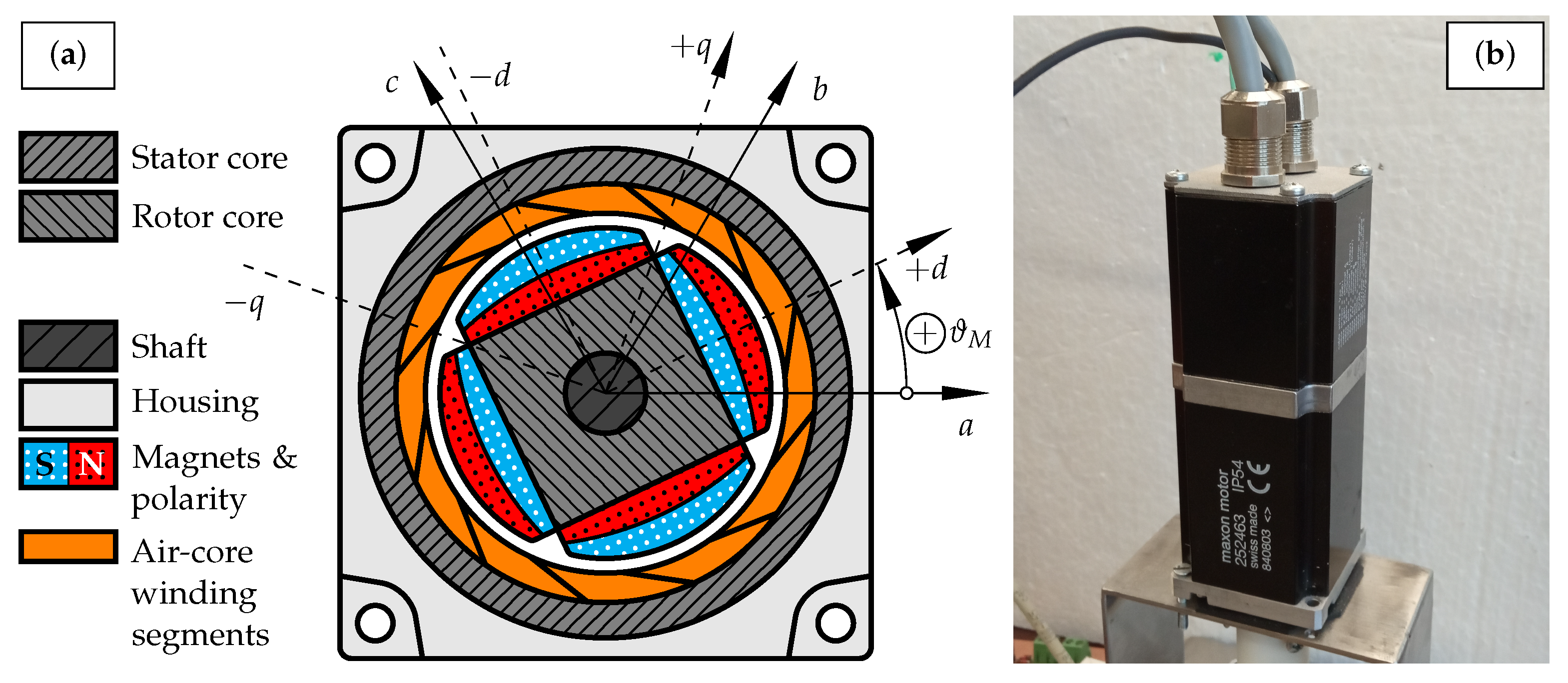
We used two Maxon EC4-pole 45 252463 slotless surface-mounted PMSMs as our test motors.

Table 1. Datasheet parameters of the Maxon EC4-pole 45 252463 type.

Parameter	Value	Parameter	Value
Nominal power	200 $\mathrm{W}$	Maximum rated continuous current	$4.16$$\mathrm{A}$
Nominal voltage	48 $\mathrm{V}$	Terminal-to-terminal resistance	878 $\mathrm{m}$$\mathsf{\Omega }$
Nominal speed	6120/$\min$	Terminal-to-terminal inductance	350 $\mathsf{\mu }$$\mathrm{H}$
Torque constant	$74.5$ $\mathrm{m}$$\mathrm{NmA}$	Rotor inertia	200 $\mathrm{g}$ $\mathrm{cm}$${}^2$
Stall torque	4070 $\mathrm{mNm}$	Mechanical time constant	$3.16$$\mathrm{ms}$
Starting current	$54.7$$\mathrm{A}$	Number of pole-pairs	2

contains the datasheet parameters and Figure 1 shows the cross-section and the photo of the motors. Important to note, the size of the factory-mounted optical encoder is comparable to the size of the motor itself.

4.2. Measurement Automation

We designed our measurement system to be able to automatically change the rotor position using a stepper motor that has a full step size of $1.8{}^{°}$ which is equivalent to a resolution of $3.6{}^{°}$ in terms of electrical angle for our two pole-pair test motors. We used the factory-mounted encoders of 13-bit resolution to correct the position error introduced by the stepper motor.

The drive control was implemented on a National Instruments CompactRIO. The low-level functions, such as the MOSFET control signal generation, current sampling, encoder signal processing and data acquisition, run on the cRIO-9104 FPGA module. The FPGA stores the measured current and rotor position values in the FIFO memory of the cRIO-9014 real-time controller which transmits the acquired current signals to our LabVIEW-based control application.

The terminal and neutral point voltages were measured using a Tektronix MSO 4054B oscilloscope. A CompactDAQ cDAQ-9188 was used as the digital output to control the stepper driver as well as trigger the data acquisition in the FPGA and the oscilloscope. The external triggering ensured the synchronized the operation of the FPGA and the oscilloscope which was required by the parameter identification method we used. We performed the voltage measurement at a higher sampling frequency in order to capture the switching transients and downsampled the voltage data to match the sampling time of the current data.

Our custom-designed and built parts include the three-phase inverter, optical coupling and current measurement circuits. Figure 2 shows a photo of our measurement environment. Figure 3 shows the types of the components used in the drive.

5. Measurement and Parameter Identification Results

We performed sinusoidal pulsating voltage injection-based measurements to acquire suitable data for the least squares estimation of the unknown machine parameters (16)–(18). The $abc$ phase voltages and currents were directly measured (see Figure 3). The $\alpha -\beta$ and $d-q$ voltages and currents were calculated using Clarke’s and Park’s transformations. The measurements were performed at zero speed.

The frequency of the pulse-width modulation was 40 $\mathrm{k}$$\mathrm{Hz}$. The sampling frequency for the current measurement was 240 $\mathrm{k}$$\mathrm{Hz}$ and we synchronized the sampling to the modulation (6 current sampling in every modulation cycle). The sampling frequency for the voltages was 10 $\mathrm{M}$$\mathrm{Hz}$ in order to capture the switching transients. The voltage signals were later downsampled to match the sampling frequency of the current data.

The frequency of the injected voltage signal was 1 $\mathrm{k}$$\mathrm{Hz}$ and its amplitude was set to $6.2$ $\mathrm{V}$. The rotor position and the injection angle were changed between each measurement. The acquired data cover all combinations of 200 rotor positions ($3.6$${}^{\circ }$ resolution in terms of electrical angle) and 18 injection angles (10${}^{\circ }$ resolution in terms of electrical angle). The duration of the signal acquisition was 10 $\mathrm{m}$$\mathrm{s}$ resulting in 2400 samples per channel i.e., time series data for 10 periods of the voltages and currents at all measurement points. Later, the 10 periods were averaged resulting in 240 samples long time series data for all measured quantities.

Figure 4 shows the voltage and current signals acquired at $\vartheta =1.36{}^{\circ }$ electrical rotor position for 18 different injection angles from 0${}^{\circ }$ to 170${}^{\circ }$ in the stationary reference frame.

5.1. Offline Ordinary Least Squares Estimation of the Machine Parameters

By substituting the quadratic flux-linkage (10) and $\omega =0$ into (2), the voltage equation that is valid at zero speed takes the form

$$\underline{u}{\phantom{u}}_{dq}=R\underline{i}{\phantom{i}}_{dq}+\underline{\underline{L}}{\phantom{L}}_{dq}\frac{\mathrm{d}{\underline{i}}_{dq}}{\mathrm{d}t}+\left(\underline{\underline{I}}{\phantom{I}}_2\otimes \underline{i}{\phantom{i}}_{dq}^T\right)\underline{\underline{\mathsf{\Gamma }}}{\phantom{\mathsf{\Gamma }}}_{dq}\frac{\mathrm{d}{\underline{i}}_{dq}}{\mathrm{d}t}.$$

(13)

After performing the matrix operations, the d- and q-direction voltage equations take the general forms

$$u_d=R{i}_d+L_{dd}\frac{\mathrm{d}{i}_d}{\mathrm{d}t}+L_{dq}\frac{\mathrm{d}{i}_q}{\mathrm{d}t}+{\displaystyle \frac{1}{2}}{\mathsf{\Gamma }}_{ddd}\frac{\mathrm{d}{i}_d^2}{\mathrm{d}t}+{\mathsf{\Gamma }}_{ddq}\frac{\mathrm{d}{i}_d{i}_q}{\mathrm{d}t}+{\displaystyle \frac{1}{2}}{\mathsf{\Gamma }}_{dqq}\frac{\mathrm{d}{i}_q^2}{\mathrm{d}t}\mathrm{and}$$

(14)

$$u_q=R{i}_q+L_{qd}\frac{\mathrm{d}{i}_d}{\mathrm{d}t}+L_{qq}\frac{\mathrm{d}{i}_q}{\mathrm{d}t}+{\displaystyle \frac{1}{2}}{\mathsf{\Gamma }}_{qdd}\frac{\mathrm{d}{i}_d^2}{\mathrm{d}t}+{\mathsf{\Gamma }}_{qdq}\frac{\mathrm{d}{i}_d{i}_q}{\mathrm{d}t}+{\displaystyle \frac{1}{2}}{\mathsf{\Gamma }}_{qqq}\frac{\mathrm{d}{i}_q^2}{\mathrm{d}t}.$$

(15)

The voltage equations are linear with respect to the unknown machine parameters and can be transformed into multiple linear regression models. The response variables are the voltages. The regressors are the currents as well as the derivatives of the currents, including the quadratic ones.

The regression models created from the d- and q-direction voltage equations are

$$\underline{u}{\phantom{u}}_d=R\underline{i}{\phantom{i}}_d+L_{dd}\underline{d}{\phantom{d}}_d+L_{dq}\underline{d}{\phantom{d}}_q+{\mathsf{\Gamma }}_{ddd}\underline{q}{\phantom{q}}_d+{\mathsf{\Gamma }}_{ddq}\underline{q}{\phantom{q}}_{dq}+{\mathsf{\Gamma }}_{dqq}\underline{q}{\phantom{q}}_q\mathrm{and}$$

(16)

$$\underline{u}{\phantom{u}}_q=R\underline{i}{\phantom{i}}_q+L_{qd}\underline{d}{\phantom{d}}_d+L_{qq}\underline{d}{\phantom{d}}_q+{\mathsf{\Gamma }}_{qdd}\underline{q}{\phantom{q}}_d+{\mathsf{\Gamma }}_{qdq}\underline{q}{\phantom{q}}_{dq}+{\mathsf{\Gamma }}_{qqq}\underline{q}{\phantom{q}}_q,$$

(17)

where $\underline{u}{\phantom{u}}_d$ and $\underline{u}{\phantom{u}}_q$ are the voltage sample vectors, $\underline{i}{\phantom{i}}_d$ and $\underline{i}{\phantom{i}}_q$ are the current sample vectors, $\underline{d}{\phantom{d}}_d$ and $\underline{d}{\phantom{d}}_q$ are the numeric derivatives of the current vectors, and the derivatives of the quadratic currents are denoted by $\underline{q}{\phantom{q}}_d$, $\underline{q}{\phantom{q}}_{dq}$ and $\underline{q}{\phantom{q}}_q$. The discretization and numeric differentiation steps are included in Appendix B.

Equations (16) and (17) are overdetermined equation systems in the forms $\underline{y}\phantom{y}=\underline{\underline{X}}\phantom{X}\underline{\beta }\phantom{\beta }$. In order to solve them, they were rearranged into the matrix forms

$$\underset{\underline{y}{\phantom{y}}_d}{\underbrace{\underline{u}{\phantom{u}}_d}}=\underset{\underline{\underline{X}}{\phantom{X}}_d}{\underbrace{\left[\begin{array}{c}\underline{i}{\phantom{i}}_d,\underline{d}{\phantom{d}}_d,\underline{d}{\phantom{d}}_q,\underline{q}{\phantom{q}}_d,\underline{q}{\phantom{q}}_{dq},\underline{q}{\phantom{q}}_q\end{array}\right]}}\underset{\underline{\beta }{\phantom{\beta }}_d}{\underbrace{\left[\begin{array}{c}R\\ L_{dd}\\ L_{dq}\\ {\mathsf{\Gamma }}_{ddd}\\ {\mathsf{\Gamma }}_{ddq}\\ {\mathsf{\Gamma }}_{dqq}\end{array}\right]}}\mathrm{and}\underset{\underline{y}{\phantom{y}}_q}{\underbrace{\underline{u}{\phantom{u}}_q}}=\underset{\underline{\underline{X}}{\phantom{X}}_q}{\underbrace{\left[\begin{array}{c}\underline{i}{\phantom{i}}_q,\underline{d}{\phantom{d}}_d,\underline{d}{\phantom{d}}_q,\underline{q}{\phantom{q}}_d,\underline{q}{\phantom{q}}_{dq},\underline{q}{\phantom{q}}_q\end{array}\right]}}\underset{\underline{\beta }{\phantom{\beta }}_q}{\underbrace{\left[\begin{array}{c}R\\ L_{qd}\\ L_{qq}\\ {\mathsf{\Gamma }}_{qdd}\\ {\mathsf{\Gamma }}_{qdq}\\ {\mathsf{\Gamma }}_{qqq}\end{array}\right]}}.$$

(18)

The best fits were calculated as ${\widehat{\beta }}_d={\left(\underline{\underline{X}}{\phantom{X}}_d^T\underline{\underline{X}}{\phantom{X}}_d\right)}^{-1}\underline{\underline{X}}{\phantom{X}}_d^T\underline{y}{\phantom{y}}_d$ and ${\widehat{\beta }}_q={\left(\underline{\underline{X}}{\phantom{X}}_q^T\underline{\underline{X}}{\phantom{X}}_q\right)}^{-1}\underline{\underline{X}}{\phantom{X}}_q^T\underline{y}{\phantom{y}}_q$.

5.2. Parameter Identification Results

The voltage and current signals acquired at a certain rotor position were concatenated to form the regressor vectors of (16) and (17). The machine parameters were calculated by solving (18). The average value of the phase resistance was $R=0.55 \mathsf{\Omega }$. Figure 5 shows the identified inductance values. The inductance values show little rotor position dependence. $L_{qq}$ is higher than $L_{dd}$. The mutual inductances $L_{dq}$ and $L_{qd}$ are negligibly small. The average values of the self-inductances are

$$L_{dd}=158\mathsf{\mu }\mathrm{H}\mathrm{and}{L}_{qq}=182\mathsf{\mu }\mathrm{H}.$$

(19)

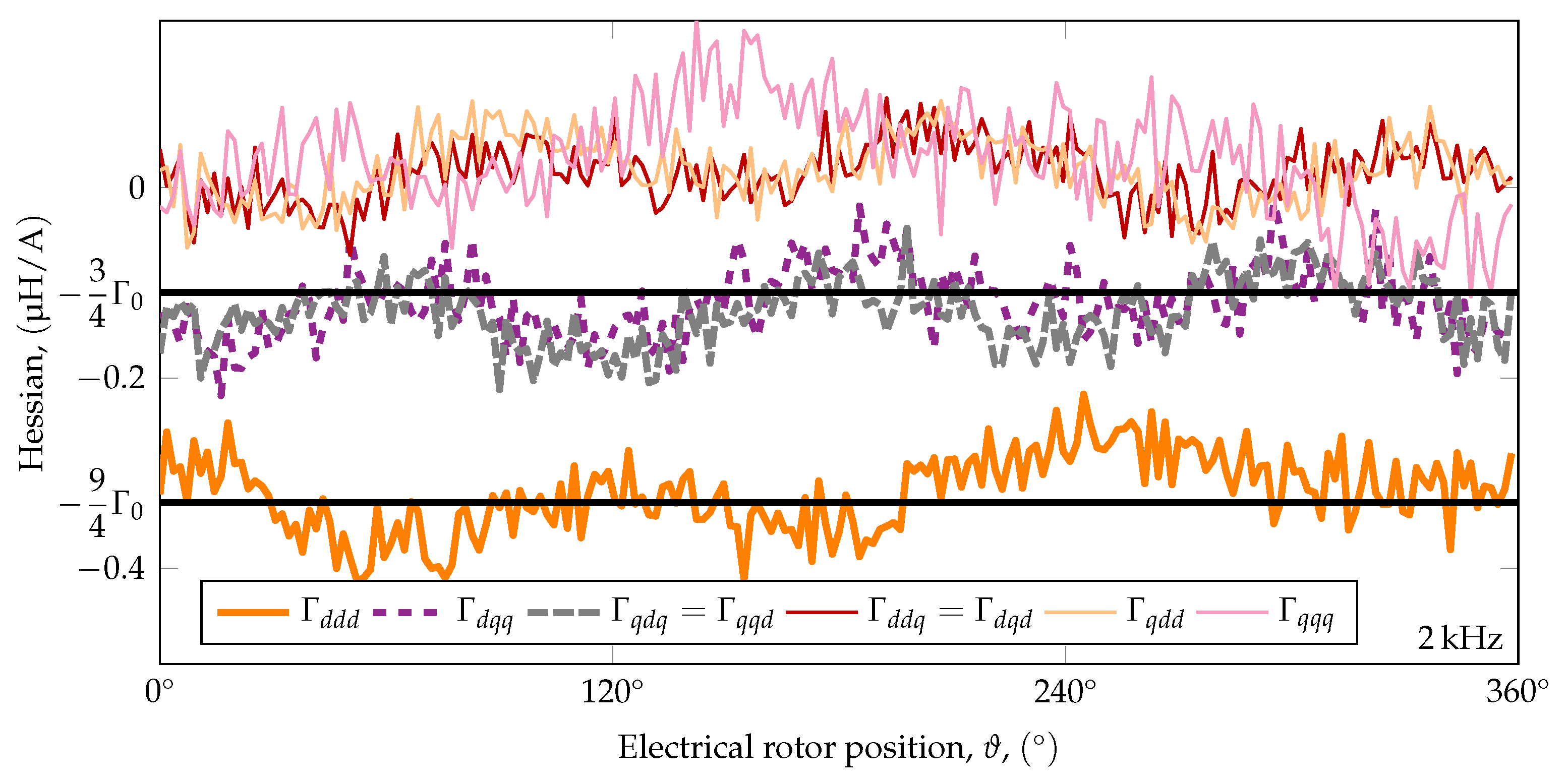
Figure 6 shows the identified values of the elements of the Hessian matrix. Their values are small and significantly noisier than the inductances but they also show little rotor position dependence. Three of the six elements are very small and we set their values to zero.

$${\mathsf{\Gamma }}_{ddq}={\mathsf{\Gamma }}_{qdd}={\mathsf{\Gamma }}_{qqq}=0\frac{\mathsf{\mu }\mathrm{H}}{\mathrm{A}}$$

(20)

Besides the $d-q$ representation, it is also important how the Hessian appears in the $\alpha -\beta$ and $abc$ coordinate systems. By introducing a new machine parameter, ${\mathsf{\Gamma }}_0$, to define the non-zero elements of $\underline{\underline{\mathsf{\Gamma }}}{\phantom{\mathsf{\Gamma }}}_{dq}$ as

$${\mathsf{\Gamma }}_{ddd}=-{\displaystyle \frac{9}{4}}{\mathsf{\Gamma }}_0=-0.281\frac{\mathsf{\mu }\mathrm{H}}{\mathrm{A}}\mathrm{and}{\mathsf{\Gamma }}_{dqq}={\mathsf{\Gamma }}_{qdq}=-{\displaystyle \frac{3}{4}}{\mathsf{\Gamma }}_0=-0.094\frac{\mathsf{\mu }\mathrm{H}}{\mathrm{A}}$$

(21)

where

$${\mathsf{\Gamma }}_0=0.125\frac{\mathsf{\mu }\mathrm{H}}{\mathrm{A}}$$

(22)

the elements of the $\alpha -\beta$ and $abc$ Hessians will have only first spatial harmonics. The idealized values defined by (21) are also plotted on Figure 6. Measurement data for 2 $\mathrm{k}$$\mathrm{Hz}$ injection frequency are included in Appendix D and

Table A1. The model parameters for 2 $\mathrm{k}$$\mathrm{Hz}$ injection frequency.

Parameter	Notation	Value
Phase resistance	R	715 $\mathrm{m}$$\mathsf{\Omega }$
d-axis self-inductance	$L_{dd}$	155 $\mathsf{\mu }$$\mathrm{H}$
q-axis self-inductance	$L_{qq}$	188 $\mathsf{\mu }$$\mathrm{H}$
Polarity dependent saliency coefficient	${\mathsf{\Gamma }}_0$	$0.146$$\frac{\mathsf{\mu }\mathrm{H}}{\mathrm{A}}$

.

Based on (19)–(21), the idealized forms of the inductance and Hessian matrices are

$$\underline{\underline{L}}{\phantom{L}}_{dq}=\left[\begin{array}{cc}{L}_{dd}& 0\\ 0& L_{qq}\end{array}\right]\mathrm{and}\underline{\underline{\mathsf{\Gamma }}}{\phantom{\mathsf{\Gamma }}}_{dq}=\left[\begin{array}{cc}-{\displaystyle \frac{9}{4}}{\mathsf{\Gamma }}_0& 0\\ 0& -{\displaystyle \frac{3}{4}}{\mathsf{\Gamma }}_0\\ 0& -{\displaystyle \frac{3}{4}}{\mathsf{\Gamma }}_0\\ -{\displaystyle \frac{3}{4}}{\mathsf{\Gamma }}_0& 0\end{array}\right].$$

(23)

The flux-linkages extended with the idealized forms of the quadratic terms are

$${\mathsf{\Psi }}_d={\mathsf{\Psi }}_{PM}+L_{dd}{i}_d-{\displaystyle \frac{9}{8}}{\mathsf{\Gamma }}_0{i}_d^2-{\displaystyle \frac{3}{8}}{\mathsf{\Gamma }}_0{i}_q^2\mathrm{and}$$

(24)

$${\mathsf{\Psi }}_q=L_{qq}{i}_q-{\displaystyle \frac{3}{4}}{\mathsf{\Gamma }}_0{i}_d{i}_q.$$

(25)

The d-axis flux-linkage is influenced by the squares of the currents, and regardless of the axis of the currents, the flux-linkage becomes lower. The q-axis flux-linkage is influenced by the product of the currents.

The phenomena described by the quadratic terms are the polarity dependent subset of main flux saturation and cross-saturation. The equations also can be interpreted as linear definitions for current dependent inductances,

$$L_{dd}^{\prime }=L_{dd}+{\displaystyle \frac{1}{2}}{\mathsf{\Gamma }}_{ddd}{i}_d=L_{dd}-{\displaystyle \frac{9}{8}}{\mathsf{\Gamma }}_0{i}_d\mathrm{and}{L}_{qq}^{\prime }=L_{qq}+{\displaystyle \frac{1}{2}}{\mathsf{\Gamma }}_{qdq}{i}_d=L_{qq}-{\displaystyle \frac{3}{8}}{\mathsf{\Gamma }}_0{i}_d.$$

(26)

6. Second Harmonic Generation Predicted by the Quadratic Flux-Linkage Extension

The main disadvantage of the linear model is the unsuitability for polarity detection. To overcome this limitation, we introduced the quadratic term of the flux-linkage in our PMSM model as described in the previous sections. The resulting nonlinear model predicts polarity dependent behavior. In this section we present the effect of the quadratic terms on the phase currents, namely the second-harmonic generation. Measurement data are also presented to demonstrate the correctness of the model.

6.1. Approximate Solution of Our Model

The voltage Equations (27) and (28) were formulated by substituting the idealized forms of the coefficient matrices (23) into (14) and (15).

$$u_d=R{i}_d+L_{dd}\frac{\mathrm{d}{i}_d}{\mathrm{d}t}-{\displaystyle \frac{9}{4}}{\mathsf{\Gamma }}_0{i}_d\frac{\mathrm{d}{i}_d}{\mathrm{d}t}-{\displaystyle \frac{3}{4}}{\mathsf{\Gamma }}_0{i}_q\frac{\mathrm{d}{i}_q}{\mathrm{d}t}$$

(27)

$$u_q=R{i}_q+L_{qq}\frac{\mathrm{d}{i}_q}{\mathrm{d}t}-{\displaystyle \frac{3}{4}}{\mathsf{\Gamma }}_0\frac{\mathrm{d}{i}_d{i}_q}{\mathrm{d}t}$$

(28)

During sinusoidal pulsating injection the voltage consists of a single harmonic with the angular frequency of ${\omega }_c$ in the form

$$\underline{u}{\phantom{u}}_{dq}=U_{0}cos\left({\omega }_{c}t\right){\mathrm{e}}^{j\gamma }=\left[\begin{array}{c}{U}_{0}cos\left({\omega }_{c}t\right)cos\left(\gamma \right)\\ U_{0}cos\left({\omega }_{c}t\right)sin\left(\gamma \right)\end{array}\right]=\left[\begin{array}{c}{u}_d\\ u_q\end{array}\right]$$

(29)

where $U_0$ is the amplitude of the injected signal, $\gamma =\delta -\vartheta$ denotes the injection angle error measured from the d axis and $\delta$ is the injection angle measured from the $\alpha$ axis.

The linear parts of the voltage equations

$$u_d=R{i}_{d\left(1\right)}+L_{dd}\frac{\mathrm{d}{i}_{d\left(1\right)}}{\mathrm{d}t}\mathrm{and}{u}_q=R{i}_{q\left(1\right)}+L_{qq}\frac{\mathrm{d}{i}_{q\left(1\right)}}{\mathrm{d}t}$$

(30)

determine the fundamental harmonics of the phase currents, $i_{d\left(1\right)}$ and $i_{q\left(1\right)}$. The parametric forms of the quasi-stationary solutions are

$$i_{d\left(1\right)}=I_{d\left(1\right)}cos\left({\omega }_{c}t+{\phi }_{d\left(1\right)}\right)\mathrm{and}{i}_{q\left(1\right)}=I_{q\left(1\right)}cos\left({\omega }_{c}t+{\phi }_{q\left(1\right)}\right),$$

(31)

where $I_{d\left(1\right)}$ and $I_{q\left(1\right)}$ are the amplitudes, ${\phi }_{d\left(1\right)}$ and ${\phi }_{q\left(1\right)}$ are the phases of the fundamental harmonics of the currents. The detailed definitions of the amplitudes and phases are included in Appendix C.

The quadratic terms of the voltage equations $-e_{d\left(2\right)}$ and $-e_{q\left(2\right)}$ act as the voltage sources for the second harmonics in the equations

$$0\mathrm{V}=R{i}_{d\left(2\right)}+L_{dd}\frac{\mathrm{d}{i}_{d\left(2\right)}}{\mathrm{d}t}\underset{-e_{d\left(2\right)}}{\underbrace{-{\displaystyle \frac{9}{4}}{\mathsf{\Gamma }}_0{i}_{d\left(1\right)}\frac{\mathrm{d}{i}_{d\left(1\right)}}{\mathrm{d}t}-{\displaystyle \frac{3}{4}}{\mathsf{\Gamma }}_0{i}_{q\left(1\right)}\frac{\mathrm{d}{i}_{q\left(1\right)}}{\mathrm{d}t}}}\mathrm{and}$$

(32)

$$0\mathrm{V}=R{i}_{q\left(2\right)}+L_{qq}\frac{\mathrm{d}{i}_{q\left(2\right)}}{\mathrm{d}t}\underset{-e_{q\left(2\right)}}{\underbrace{-{\displaystyle \frac{3}{4}}{\mathsf{\Gamma }}_0\frac{\mathrm{d}{i}_{d\left(1\right)}{i}_{q\left(1\right)}}{\mathrm{d}t}}}.$$

(33)

Expressing $e_{d\left(2\right)}$ and $e_{q\left(2\right)}$ by substituting the fundamental harmonics of the currents (31) reveals that their angular frequency is $2{\omega }_c$.

$$e_{d\left(2\right)}={\displaystyle \frac{9}{8}}{\mathsf{\Gamma }}_0{I}_{d\left(1\right)}^2{\omega }_{c}sin\left(2{\omega }_{c}t+2{\phi }_{d\left(1\right)}\right)+{\displaystyle \frac{3}{8}}{\mathsf{\Gamma }}_0{I}_{q\left(1\right)}^2{\omega }_{c}sin\left(2{\omega }_{c}t+2{\phi }_{q\left(1\right)}\right)$$

(34)

$$e_{q\left(2\right)}={\displaystyle \frac{3}{4}}{\mathsf{\Gamma }}_0{I}_{d\left(1\right)}{I}_{q\left(1\right)}{\omega }_{c}sin\left(2{\omega }_{c}t+{\phi }_{d\left(1\right)}+{\phi }_{q\left(1\right)}\right)$$

(35)

The inductive-resistive linear parts of the model filter $e_{d\left(2\right)}$ and $e_{q\left(2\right)}$ to produce the second harmonics of the currents, $i_{d\left(2\right)}$ and $i_{q\left(2\right)}$, respectively. The additional phase shifts ${\eta }_{d\left(2\right)}$ and ${\eta }_{q\left(2\right)}$ corresponding to $2{\omega }_c$ angular frequency are

$${\eta }_{d\left(2\right)}=arctan\left({\displaystyle \frac{R}{2{\omega }_c{L}_{dd}}}\right)\mathrm{and}{\eta }_{q\left(2\right)}=arctan\left({\displaystyle \frac{R}{2{\omega }_c{L}_{qq}}}\right).$$

(36)

The detailed definitions of the phase shifts that take into account the ambiguity introduced by inductance tracking, are included in Appendix C.

The quasi-stationary solutions of (32) and (33) are the second harmonics of the currents,

$$i_{d\left(2\right)}={\displaystyle \frac{9}{8}}{\displaystyle \frac{I_{d\left(1\right)}^2\left|{\mathsf{\Gamma }}_0\right|cos\left(2{\omega }_{c}t+2{\phi }_{d\left(1\right)}+{\eta }_{d\left(2\right)}\right)}{\sqrt{R^2+4{\omega }_c^2{L}_{dd}^2}}}+{\displaystyle \frac{3}{8}}{\displaystyle \frac{I_{q\left(1\right)}^2\left|{\mathsf{\Gamma }}_0\right|cos\left(2{\omega }_{c}t+2{\phi }_{q\left(1\right)}+{\eta }_{d\left(2\right)}\right)}{\sqrt{R^2+4{\omega }_c^2{L}_{dd}^2}}}$$

(37)

$$\mathrm{and}{i}_{q\left(2\right)}={\displaystyle \frac{3}{4}}{\displaystyle \frac{I_{d\left(1\right)}{I}_{q\left(1\right)}\left|{\mathsf{\Gamma }}_0\right|cos\left(2{\omega }_{c}t+{\phi }_{d\left(1\right)}+{\phi }_{q\left(1\right)}+{\eta }_{q\left(2\right)}\right)}{\sqrt{R^2+{\omega }_c^2{L}_{qq}^2}}}.$$

(38)

To conclude this section, the inductive-resistive linear part of the model produces the fundamental harmonics of the response currents. Then the quadratic terms act as frequency doubling inner voltage sources. Finally, as a response to $e_{d\left(2\right)}$ and $e_{q\left(2\right)}$, the linear part produces the second harmonics of the currents, $i_{d\left(2\right)}$ and $i_{q\left(2\right)}$.

6.2. Validation of the Second Harmonic Generation

Our quadratic model extension predicts the second harmonic content of the d- and q-axis currents, (37) and (38). The second harmonics can be rearranged into forms

$$i_{d\left(2\right)}=I_{d\left(2\right)}cos(2{\omega }_{c}t+{\phi }_{d\left(2\right)})\mathrm{and}{i}_{q\left(2\right)}=I_{q\left(2\right)}cos(2{\omega }_{c}t+{\phi }_{q\left(2\right)}),$$

(39)

where $I_{d\left(2\right)}$ and $I_{q\left(2\right)}$ are the amplitudes, ${\phi }_{d\left(2\right)}$ and ${\phi }_{q\left(2\right)}$ are the phases of the second harmonics of the currents. The detailed definitions of the amplitudes and phases are included in Appendix C, (A12)–(A15).

The amplitudes and phases of the second harmonics are not constant values, they depend on the injection angle error $\gamma$ and indirectly on the rotor position $\vartheta$. We analyzed these properties to prove the correctness of our model extension.

Figure 7, Figure 8, Figure 9 and Figure 10 show the measured values of the amplitudes and phases, and compare them to the values predicted by the model. The measurement data are plotted as surfaces against the independent variables of the measurement. The comparison charts are plotted against the $\gamma$ injection angle error, which is equal to the difference between the injection angle in the stationary reference frame $\delta$ and the electrical rotor position $\vartheta$.

In this section we reused the pulsating injection measurement data acquired for the parameter identification where the amplitude of the injected voltage signal was $6.2$ $\mathrm{V}$. To put the amplitude values into context, the amplitudes of the fundamental harmonics of the currents were between $4.7$ $\mathrm{A}$ and 6 $\mathrm{A}$ and the standard deviation of the current measurement was ${\sigma }_{CM}=4.4 \mathrm{m}\mathrm{A}$. The amplitude and phase values were produced by discrete Fourier-transforming the current signals.

Figure 7 shows the amplitude of the second harmonic of the d-axis current, $I_{d\left(2\right)}$. Our model correctly predicts the values and the injection angle error dependency of $I_{d\left(2\right)}$ in the 4–$15 \mathrm{m}\mathrm{A}$ range, although there are certain $\delta$-$\vartheta$ combinations where we can see systematic deviations from the model. Important to note that the current values were quiet high for our test motors yet the polarity dependent second harmonics were very small compared to the first harmonics. Figure 8 shows the phase of the second harmonic of the d-axis current, ${\phi }_{d\left(2\right)}$. The phase value is less noisy during injection in the $+d$ and $-d$ directions where the $I_{d\left(2\right)}$ amplitude is higher and the phase value becomes unreliable when the injection happens in the $+q$ or $-q$ directions.

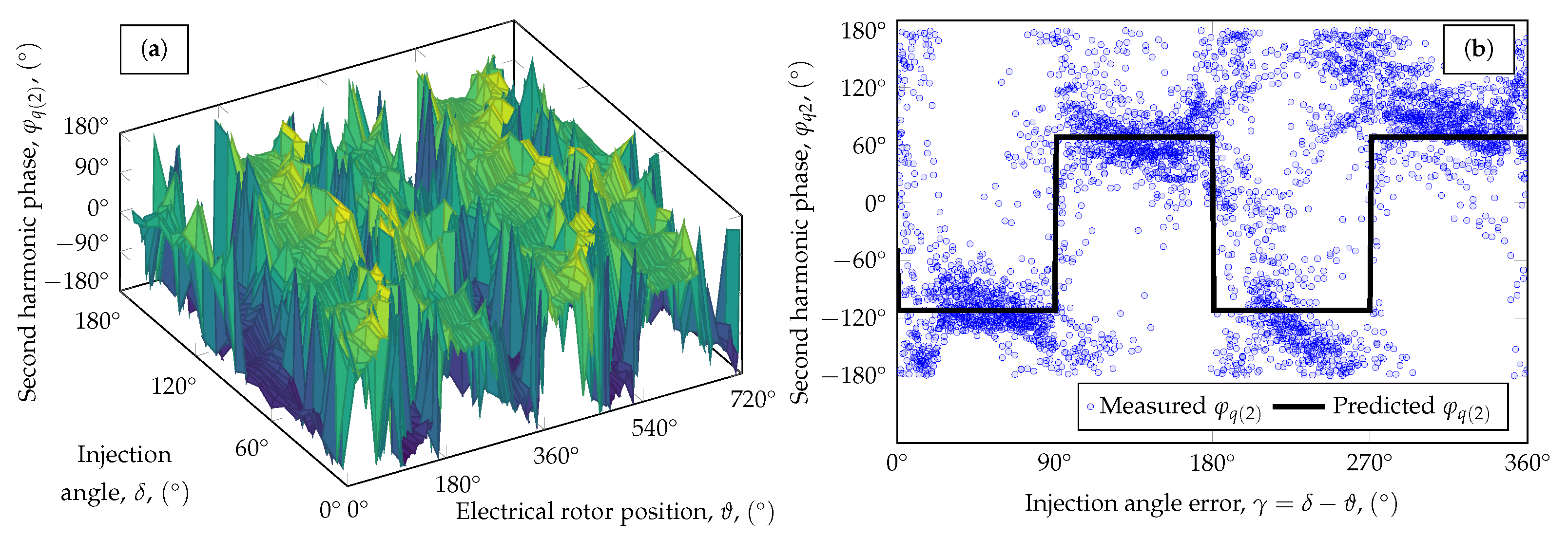
Figure 9 and Figure 10 show the parameters of the second harmonic of the q-axis current. The measurement results are much noisier than the d-direction results. The amplitude predicted by the model is smaller than ${\sigma }_{CM}=4.4 \mathrm{m}\mathrm{A}$ and the injection angle error dependence of $I_{q\left(2\right)}$ is unclear. The ${\phi }_{q\left(2\right)}$ phase data are also noisy, however, a large number of the samples are in clusters around the predicted values.

We also performed measurements at 7 different injected voltage amplitudes. In these measurements, the voltage signals were injected in the d-direction and the measurement was repeated at 25 evenly distributed rotor positions. We analyzed the relationship between the amplitude of the fundamental harmonic and the properties of the second harmonic of the d-axis current. Figure 11 shows the measured and predicted amplitudes and phases of the second harmonic for different $I_{d\left(1\right)}$ values.

The relationship between the amplitudes of the fundamental and second harmonics of the d-axis current is quadratic and can be written in the form

$$I_{d\left(2\right)}={\displaystyle \frac{9}{4}}{\displaystyle \frac{{\omega }_c{\mathsf{\Gamma }}_0}{\sqrt{R^2+4{\omega }_c^2{L}_{dd}^2}}}{I}_{d\left(1\right)}^2$$

(40)

when the injection angle error $\gamma =0$ and consequently $I_{q\left(1\right)}=0\mathrm{A}$. Under the same circumstances, the phase of the second harmonic of the d-axis current is equal to

$${\phi }_{d\left(2\right)}=2{\phi }_{d\left(1\right)}+{\eta }_{d\left(2\right)}.$$

(41)

The model parameters for 1 $\mathrm{k}$$\mathrm{Hz}$ injection frequency are listed in

Table 2. The model parameters for 1$\mathrm{k}$$\mathrm{Hz}$ injection frequency.

Parameter	Notation	Value
Phase resistance	R	550 $\mathrm{m}$$\mathsf{\Omega }$
d-axis self-inductance	$L_{dd}$	158 $\mathsf{\mu }$$\mathrm{H}$
q-axis self-inductance	$L_{qq}$	182 $\mathsf{\mu }$$\mathrm{H}$
Polarity dependent saliency coefficient	${\mathsf{\Gamma }}_0$	$0.125$$\frac{\mathsf{\mu }\mathrm{H}}{\mathrm{A}}$

.

6.3. Separated Forms of the Voltage Equations

The model defined by (27) and (28) is a separable nonlinear differential equation system. We are not aware of a general analytical solution for arbitrary $u_d$ and $u_q$ voltage inputs. Therefore, we developed a form of the model that is more suitable for numerical simulation by separating the variables of (27) and (28) as can be seen in (42) and (43).

$$\frac{\mathrm{d}{i}_d}{\mathrm{d}t}={\displaystyle \frac{\left(L_{qq}-{\displaystyle \frac{3}{4}}{\mathsf{\Gamma }}_0{i}_d\right)\left(u_d-R{i}_d\right)+{\displaystyle \frac{3}{4}}{\mathsf{\Gamma }}_0{i}_q\left(u_q-R{i}_q\right)}{\left(L_{dd}-{\displaystyle \frac{9}{4}}{\mathsf{\Gamma }}_0{i}_d\right)\left(L_{qq}-{\displaystyle \frac{3}{4}}{\mathsf{\Gamma }}_0{i}_d\right)-{\displaystyle \frac{9}{16}}{\mathsf{\Gamma }}_0^2{i}_q^2}}$$

(42)

$$\frac{\mathrm{d}{i}_q}{\mathrm{d}t}={\displaystyle \frac{\left(L_{dd}-{\displaystyle \frac{9}{4}}{\mathsf{\Gamma }}_0{i}_d\right)\left(u_q-R{i}_q\right)-{\mathsf{\Gamma }}_{qdq}{i}_q\left(u_d-R{i}_d\right)}{\left(L_{dd}-{\displaystyle \frac{9}{4}}{\mathsf{\Gamma }}_0{i}_d\right)\left(L_{qq}-{\displaystyle \frac{3}{4}}{\mathsf{\Gamma }}_0{i}_d\right)-{\displaystyle \frac{9}{16}}{\mathsf{\Gamma }}_0^2{i}_q^2}}$$

(43)

The domain of the differential equation system is limited by the divisions. In the case of our test motors, the absolute value of $i_q$ must be smaller than 1808 $\mathrm{A}$ to avoid division by zero, which is much higher than the physically realizable current, and therefore, does not provide a practical limitation.

7. Polarity Detection Based on the Second Harmonic of the $\mathit{D}$-Axis Current

Polarity detection is performed in the initial position detection phase after the saliency tracking algorithm found the $+d$ or the $-d$ axis. At that point the estimated rotor position is either $\widehat{\vartheta }\approx \vartheta$ (i.e., $\gamma \approx 0$) or $\widehat{\vartheta }\approx \vartheta +\pi$ (i.e., $\gamma \approx \pi$). The inductance matrices of the correct $+d/+q$ and opposite $-d/-q$ coordinate systems are equal because

$$\underline{\underline{L}}{\phantom{L}}_{dq}^{\mathrm{opposite}}=\underline{\underline{T}}\phantom{T}\left(\vartheta +\pi \right)\underline{\underline{L}}{\phantom{L}}_{\alpha \beta }\left(\vartheta \right)\underline{\underline{T}}{\phantom{T}}^{-1}\left(\vartheta +\pi \right)=\left[\begin{array}{cc}{L}_{dd}& 0\\ 0& L_{qq}\end{array}\right]=\underline{\underline{L}}{\phantom{L}}_{dq}.$$

(44)

Therefore, the inductance-based algorithms cannot distinguish between +d/+q and opposite $-d/-q$ coordinate systems.

The Hessian matrix, however, which takes the form

$$\underline{\underline{\mathsf{\Gamma }}}{\phantom{\mathsf{\Gamma }}}_{\alpha \beta }\left(\vartheta \right)=\left(\underline{\underline{I}}{\phantom{I}}_2\otimes \underline{\underline{T}}{\phantom{T}}^T\left(\vartheta \right)\right)\left(\underline{\underline{T}}{\phantom{T}}^{-1}\left(\vartheta \right)\otimes \underline{\underline{I}}{\phantom{I}}_2\phantom{\underline{\underline{T}}\phantom{T}\left(\vartheta \right)}\right)\underline{\underline{\mathsf{\Gamma }}}{\phantom{\mathsf{\Gamma }}}_{dq}\underline{\underline{T}}\phantom{T}\left(\vartheta \right)=-{\displaystyle \frac{3}{4}}{\mathsf{\Gamma }}_0\left[\begin{array}{cc}3cos\vartheta & sin\vartheta \\ sin\vartheta & cos\vartheta \\ sin\vartheta & cos\vartheta \\ cos\vartheta & 3sin\vartheta \end{array}\right]$$

(45)

in the $\alpha -\beta$ coordinate system, behaves differently. In the opposite $-d/-q$ coordinate system (i.e., $\gamma \approx \pi$), the opposite Hessian is

$$\underline{\underline{\mathsf{\Gamma }}}{\phantom{\mathsf{\Gamma }}}_{dq}^{\mathrm{opposite}}=\left(\underline{\underline{I}}{\phantom{I}}_2\otimes \underline{\underline{T}}{\phantom{T}}^{T-1}\left(\vartheta +\pi \right)\right)\left(\underline{\underline{T}}\phantom{T}\left(\vartheta +\pi \right)\otimes \underline{\underline{I}}{\phantom{I}}_2\right)\underline{\underline{\mathsf{\Gamma }}}{\phantom{\mathsf{\Gamma }}}_{\alpha \beta }\left(\vartheta \right)\underline{\underline{T}}{\phantom{T}}^{-1}\left(\vartheta +\pi \right)=-\underline{\underline{\mathsf{\Gamma }}}{\phantom{\mathsf{\Gamma }}}_{dq},$$

(46)

which is the opposite of $\underline{\underline{\mathsf{\Gamma }}}{\phantom{\mathsf{\Gamma }}}_{dq}$. Then the motor behaves like if its ${\mathsf{\Gamma }}_0^{\mathrm{opposite}}$ parameter were equal to $-{\mathsf{\Gamma }}_0$. The quadratic terms of the voltage Equations (34) and (35) are affected by the sign change and the second harmonics of the currents undergo an additional 180 ${}^{\circ }$ phase change (A11). As a consequence, the magnet polarity can be determined based on the phase of the second harmonic of the d-axis current. It should be noted that it would be possible to use a signed amplitude instead of a phase change. In addition, the injection in the $-d$-direction is equivalent to $\gamma =180{}^{\circ }$ injection angle error in the correct $+d/+q$ coordinate system.

We can decide if the coordinate system is $+d/+q$ or $-d/-q$ based on the phase of $i_{d\left(2\right)}$. However, it is impractical to use the voltage signal as phase reference because the drive electronics introduce an unknown time delay between the digital I/O ports and the motor windings. Instead, the fundamental harmonic of the d-axis current is used as reference signal and the polarity-dependent quantity is

$$\mathsf{\Delta }{\phi }_{d\left(2\right)}={\phi }_{d\left(2\right)}-2{\phi }_{d\left(1\right)}$$

(47)

which is the phase difference between the second and the fundamental harmonic of $i_d$. Based on (A13) the phase differences are

$$\mathsf{\Delta }{\phi }_{d\left(2\right)}\left(\gamma =0\right)={\eta }_{d\left(2\right)}\mathrm{and}\mathsf{\Delta }{\phi }_{d\left(2\right)}\left(\gamma =\pi \right)={\eta }_{d\left(2\right)}-\pi .$$

(48)

Figure 12 shows the measured current as well as the measured and predicted second harmonics for $\gamma =0$ and $\gamma =\pi$. The measured $i_{d\left(2\right)}$ curves are in fact the even harmonic contents of the current signals.

7.1. The Properties of the Apparent D-Axis Current

The injection angle error is not guaranteed to be exactly 0 or $\pi$ during polarity detection. The apparent current vector $\underline{\widehat{\mathit{ı}}}{\phantom{\widehat{\mathit{ı}}}}_d$ measured in the estimated $d-q$ system is a projection of the actual $\underline{i}{\phantom{i}}_{dq}$ current vector that takes the form

$$\underline{\widehat{\mathit{ı}}}{\phantom{\widehat{\mathit{ı}}}}_{dq}=\underline{\underline{R}}\phantom{R}\left(-\gamma \right)\underline{i}{\phantom{i}}_{dq}=\left[\begin{array}{cc}cos\gamma & sin\gamma \\ -sin\gamma & cos\gamma \end{array}\right]\left[\begin{array}{c}{i}_d\\ i_q\end{array}\right]$$

(49)

from where the apparent d-axis current is

$${\widehat{\mathit{ı}}}_d=i_{d}cos\gamma +i_{q}sin\gamma .$$

(50)

The phase difference between the second and fundamental harmonic of ${\widehat{\mathit{ı}}}_d$ is

$$\mathsf{\Delta }{\widehat{\phi }}_{d\left(2\right)}={\widehat{\phi }}_{d\left(2\right)}-2{\widehat{\phi }}_{d\left(1\right)},$$

(51)

where ${\widehat{\phi }}_{d\left(1\right)}$ and ${\widehat{\phi }}_{d\left(2\right)}$ are the phases of the fundamental and second harmonics of ${\widehat{\mathit{ı}}}_d$. The detailed definitions of the amplitudes and phases are included in Appendix C.3, (A16)–(A19).

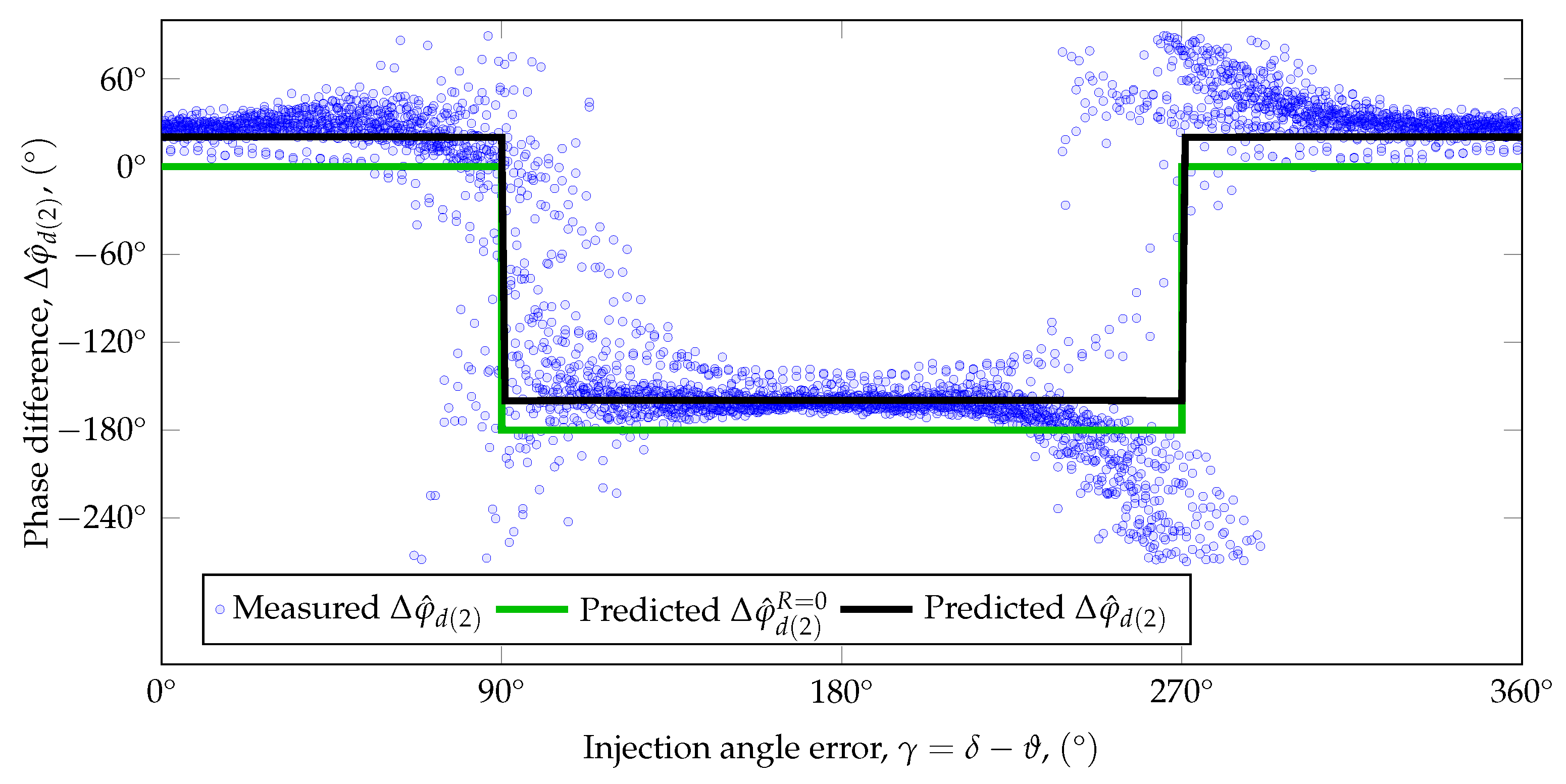
Figure 13 shows the measured and predicted values of the apparent phase difference. Our model reliably predicts the phase difference. The data show that polarity detection is the most reliable around the $+d$ and $-d$ directions.

7.2. Comparison to a Purely Inductive Model

Figure 12 and Figure 13 also show the predicted second harmonics and phase difference for the case of neglected phase resistance ($i_{d\left(2\right)}^{R=0}$ and $\mathsf{\Delta }{\widehat{\phi }}_{d\left(2\right)}^{R=0}$, both plotted in green). The phase difference $\mathsf{\Delta }{\widehat{\phi }}_{d\left(2\right)}^{R=0}$ is equal to 0 ${}^{\circ }$ at the north pole and $-180$${}^{\circ }$ at the south pole which are equivalent to the phase differences estimated based on [4,35,36]. Compared to the measured values, the error of the purely inductive model is $23.5$${}^{\circ }$. The proposed model, taking into account the phase resistance, provides a better prediction for the phase of the second harmonic, and the error is about $3.2$${}^{\circ }$.

References [4,35,36] do not quantify the coefficients of the quadratic term and therefore cannot be used to estimate the amplitude of $i_{d\left(2\right)}$. To evaluate the effect of the neglected phase resistance, we set R to zero in the proposed model to calculate $i_{d\left(2\right)}^{R=0}$. The purely inductive model slightly overestimates the amplitude of $i_{d\left(2\right)}$. The proposed model accurately predicts the polarity dependent second harmonic of $i_d$ for pulsating sinusoidal voltage injection.

7.3. Sensorless Polarity Detection Based on D-Direction Pulsating Injection

Figure 14 shows the signal processing system we designed for initial position detection that is capable of extracting the polarity information from the measured phase currents. The system is a combined and modified version of [12,26,35]. The two main components of the initial position detection algorithm are the d-axis tracking and the polarity detection that are based on coherent amplitude demodulation. The coherent reference signal generation requires synchronization to the apparent d-axis current which is achieved by the phase detection subsystem that calculates ${\widehat{\phi }}_{d\left(1\right)}$, the phase of the fundamental harmonic of the apparent d-axis current. The phase detection is based on I/Q-demodulation and complex argument calculation. In our implementation ${\widehat{\phi }}_{d\left(1\right)}$ is constant, and therefore it is determined only once at startup before d-axis search and polarity detection.

The coherent amplitude demodulation algorithm applied in the polarity detection subsystem uses $r_2\left(t\right)=cos\left(2{\omega }_{c}t+{\alpha }_2\right)$ as reference signal. The output of the demodulation is proportional to the $L^2$-inner product of ${\widehat{\mathit{ı}}}_d$ and $r_2$,

$$\langle {\widehat{\mathit{ı}}}_d,r_2\rangle =\underset{0}{\overset{T}{\int }}{\widehat{I}}_{d\left(2\right)}cos(2{\omega }_{c}t+{\phi }_{d\left(2\right)})cos\left(2{\omega }_{c}t+{\alpha }_2\right)\mathrm{d}t={\displaystyle \frac{{\widehat{I}}_{d\left(2\right)}\pi cos({\phi }_{d\left(2\right)}-{\alpha }_2)}{2{\omega }_c}}$$

(52)

where $2{\omega }_{c}T=2\pi$. To maximize its absolute value, ${\alpha }_2$ has to be set to

$${\alpha }_2={\phi }_{d\left(2\right)}\approx 2{\widehat{\phi }}_{d\left(1\right)}+{\eta }_{d\left(2\right)}$$

(53)

The ${\eta }_{d\left(2\right)}$ and ${\phi }_{q\left(1\right)}-{\phi }_{d\left(1\right)}$ phase shifts are constant values and has to be precomputed using (36), (A9) and (A10) by substituting $\gamma =0$. The output of the demodulation in the polarity detection subsystem is positive in the $+d/+q$ system and negative in the $-d/-q$. The value of $\epsilon$ is zero in the former case, whereas $\pi$ in the latter case.

In the case of our test motors, the measurement results plotted in Figure 13 show that ${\eta }_{d\left(2\right)}=23.5{}^{\circ }$. The proposed model predicts ${\eta }_{d\left(2\right)}=20.25{}^{\circ }$, while a purely inductive model predicts ${\eta }_{d\left(2\right)}=0{}^{\circ }$. This means that the proposed model provides better phase coherence. The output of the demodulation is 99.8% of the theoretical maximum for the proposed model and 91.7% for the purely inductive model. The better phase coherence results in slightly better performance in noisy environment and faster polarity detection.

8. Conclusions

In this article, a quadratic flux-linkage model extension was presented for the sensorless control of PMSM drives. The purpose of the model extension was to accurately predict the polarity-dependent second harmonic content of the motor currents. The model extension is based on the Taylor series expansion of the flux-linkage function. It does not introduce discontinuities and is not limited to the d-direction. The model extension introduces a new machine parameter, the polarity-dependent saliency coefficient ${\mathsf{\Gamma }}_0$, which describes the susceptibility of the machine to polarity-dependent saturation. The parameters of the extended machine model were determined by measurements.

We provide an approximate analytical solution of the proposed machine model for sinusoidal pulsating voltage injection where the phase resistances are not neglected. The model predicts polarity dependent second harmonic generation. The article presents measurement data showing that the predicted amplitudes and phases of the second harmonics are correct. Data for the comparison of the proposed model and a purely inductive model is also presented. It is shown that the proposed model provides more accurate prediction of the phase difference between the fundamental and second harmonics of the d-axis current. The proposed model also provides formulae for the calculation the amplitude of the second harmonics. Both the presented measurement data and the proposed model show that injection in the d-direction is optimal for polarity detection. Polarity detection using q-direction injection is impractical.

In future research work, we plan to analyze the frequency dependence of ${\mathsf{\Gamma }}_0$ and investigate the existence of an optimal injection frequency for polarity detection. Moreover, we plan to measure the Hessians of other PMSM types to see if the constants introduced in (21) are machine specific.

References

- De Kock, H.W.; Kamper, M.J.; Kennel, R.M. Anisotropy comparison of reluctance and PM synchronous machines for position sensorless control using HF carrier injection. IEEE Trans. Power Electron. 2009, 24, 1905–1913. [Google Scholar] [CrossRef]
- Rind, S.J.; Jamil, M.; Amjad, A. Electric Motors and Speed Sensorless Control for Electric and Hybrid Electric Vehicles: A Review. In Proceedings of the 2018 53rd International Universities Power Engineering Conference (UPEC), Scotland, UK, 4–7 September 2018; pp. 1–6. [Google Scholar] [CrossRef]
- Tan, L.N.; Cong, T.P.; Cong, D.P. Neural Network Observers and Sensorless Robust Optimal Control for Partially Unknown PMSM With Disturbances and Saturating Voltages. IEEE Trans. Power Electron. 2021, 36, 12045–12056. [Google Scholar] [CrossRef]
- Jeong, Y.S.; Lorenz, R.; Jahns, T.; Sul, S.K. Initial rotor position estimation of an interior permanent-magnet synchronous machine using carrier-frequency injection methods. IEEE Trans. Ind. Appl. 2005, 41, 38–45. [Google Scholar] [CrossRef] [Green Version]
- Zhao, Y.; Yu, H.; Wang, S. An Improved Super-Twisting High-Order Sliding Mode Observer for Sensorless Control of Permanent Magnet Synchronous Motor. Energies 2021, 14, 6047. [Google Scholar] [CrossRef]
- Bojoi, R.; Pastorelli, M.; Bottomley, J.; Giangrande, P.; Gerada, C. Sensorless control of PM motor drives—A technology status review. In Proceedings of the 2013 IEEE Workshop on Electrical Machines Design, Control and Diagnosis (WEMDCD), Paris, France, 11–12 March 2013; pp. 168–182. [Google Scholar] [CrossRef]
- Wei, J.; Xu, H.; Zhou, B.; Zhang, Z.; Gerada, C. An Integrated Method for Three-Phase AC Excitation and High-Frequency Voltage Signal Injection for Sensorless Starting of Aircraft Starter/Generator. IEEE Trans. Ind. Electron. 2019, 66, 5611–5622. [Google Scholar] [CrossRef]
- Hua, Y.; Zhu, H. Sensorless Control of Bearingless Permanent Magnet Synchronous Motor Based on LS-SVM Inverse System. Electronics 2021, 10, 265. [Google Scholar] [CrossRef]
- Lehmann, O.; Schuster, J.; Roth-Stielow, J. Sensorless Control Techniques as Redundancy for the Control of Permanent Magnet Synchronous Machines in Electric Vehicles. In Proceedings of the 2014 IEEE Vehicle Power and Propulsion Conference (VPPC), Coimbra, Portugal, 27–30 October 2014; pp. 1–6. [Google Scholar] [CrossRef]
- Jarzebowicz, L.; Karwowski, K.; Kulesza, W.J. Sensorless algorithm for sustaining controllability of IPMSM drive in electric vehicle after resolver fault. Control Eng. Pract. 2017, 58, 117–126. [Google Scholar] [CrossRef]
- Briz, F.; Degner, M.W. Rotor position estimation—A review of high-frequency methods. IEEE Ind. Electron. Mag. 2011, 5, 24–36. [Google Scholar] [CrossRef]
- Holtz, J. Initial rotor polarity detection and sensorless control of PM synchronous machines. In Proceedings of the Conference Record of the 2006 IEEE Industry Applications Conference Forty-First IAS Annual Meeting, Tampa, FL, USA, 8–12 October 2006; Volume 4, pp. 2040–2047. [Google Scholar] [CrossRef]
- Liu, Y.; Fang, J.; Tan, K.; Huang, B.; He, W. Sliding Mode Observer with Adaptive Parameter Estimation for Sensorless Control of IPMSM. Energies 2020, 13, 5991. [Google Scholar] [CrossRef]
- Marchesoni, M.; Passalacqua, M.; Vaccaro, L.; Calvini, M.; Venturini, M. Performance improvement in a sensorless surface-mounted PMSM drive based on rotor flux observer. Control Eng. Pract. 2020, 96, 104276–104286. [Google Scholar] [CrossRef]
- Dilys, J.; Stankevič, V.; Łuksza, K. Implementation of Extended Kalman Filter with Optimized Execution Time for Sensorless Control of a PMSM Using ARM Cortex-M3 Microcontroller. Energies 2021, 14, 3491. [Google Scholar] [CrossRef]
- Vas, P. Sensorless Vector and Direct Torque Control; Monographs in Electrical and Electronic Engineering; Oxford University Press: Oxford, UK, 1998. [Google Scholar]
- Wang, G.; Valla, M.; Solsona, J. Position Sensorless Permanent Magnet Synchronous Machine Drives—A Review. IEEE Trans. Ind. Electron. 2020, 67, 5830–5842. [Google Scholar] [CrossRef]
- Bianchi, N.; Bolognani, S.; Jang, J.H.; Sul, S.K. Comparison of PM Motor Structures and Sensorless Control Techniques for Zero-Speed Rotor Position Detection. IEEE Trans. Power Electron. 2007, 22, 2466–2475. [Google Scholar] [CrossRef]
- Xu, D.; Wang, B.; Zhang, G.; Wang, G.; Yu, Y. A review of sensorless control methods for AC motor drives. CES Trans. Electr. Mach. Syst. 2018, 2, 104–115. [Google Scholar] [CrossRef]
- Guo, L.; Yang, Z.; Lin, F. A Novel Strategy for Sensorless Control of IPMSM with Error Compensation Based on Rotating High Frequency Carrier Signal Injection. Energies 2020, 13, 1919. [Google Scholar] [CrossRef]
- Linke, M.; Kennel, R.; Holtz, J. Sensorless position control of permanent magnet synchronous machines without limitation at zero speed. In Proceedings of the IEEE 2002 28th Annual Conference of the Industrial Electronics Society, Sevilla, Spain, 5–8 November 2002; Volume 1, pp. 674–679. [Google Scholar] [CrossRef]
- Zhao, C.; Tanaskovic, M.; Percacci, F.; Mariéthoz, S.; Gnos, P. Sensorless Position Estimation for Slotless Surface Mounted Permanent Magnet Synchronous Motors in Full Speed Range. IEEE Trans. Power Electron. 2019, 34, 11566–11579. [Google Scholar] [CrossRef]
- Wang, Z.; Yao, B.; Guo, L.; Jin, X.; Li, X.; Wang, H. Initial Rotor Position Detection for Permanent Magnet Synchronous Motor Based on High-Frequency Voltage Injection without Filter. World Electr. Veh. J. 2020, 11, 71. [Google Scholar] [CrossRef]
- Szalay, I.; Kohlrusz, G.; Fodor, D. Modeling of slotless surface-mounted PM synchronous motor for sensorless applications. In Proceedings of the 2014 IEEE International Electric Vehicle Conference, Florence, Italy, 17–19 December 2014; pp. 1–5. [Google Scholar] [CrossRef]
- Murakami, S.; Shiota, T.; Ohto, M.; Ide, K.; Hisatsune, M. Encoderless Servo Drive With Adequately Designed IPMSM for Pulse-Voltage-Injection-Based Position Detection. IEEE Trans. Ind. Appl. 2012, 48, 1922–1930. [Google Scholar] [CrossRef]
- Kim, H.; Huh, K.K.; Lorenz, R.; Jahns, T. A novel method for initial rotor position estimation for IPM synchronous machine drives. IEEE Trans. Ind. Appl. 2004, 40, 1369–1378. [Google Scholar] [CrossRef] [Green Version]
- Nakashima, S.; Inagaki, Y.; Miki, I. Sensorless initial rotor position estimation of surface permanent-magnet synchronous motor. IEEE Trans. Ind. Appl. 2000, 36, 1598–1603. [Google Scholar] [CrossRef]
- Wang, Z.; Cao, Z.; He, Z. Improved Fast Method of Initial Rotor Position Estimation for Interior Permanent Magnet Synchronous Motor by Symmetric Pulse Voltage Injection. IEEE Access 2020, 8, 59998–60007. [Google Scholar] [CrossRef]
- Tursini, M.; Petrella, R.; Parasiliti, F. Initial rotor position estimation method for PM motors. IEEE Trans. Ind. Appl. 2003, 39, 1630–1640. [Google Scholar] [CrossRef]
- Lee, W.J.; Sul, S.K. A New Starting Method of BLDC Motors Without Position Sensor. IEEE Trans. Ind. Appl. 2006, 42, 1532–1538. [Google Scholar] [CrossRef]
- Hu, H.; Xu, G.; Hu, B. A New Start Method for Sensorless Brushless DC Motor Based on Pulse Injection. In Proceedings of the 2009 Asia-Pacific Power and Energy Engineering Conference, Wuhan, China, 28–30 March 2009; pp. 1–5. [Google Scholar] [CrossRef]
- Bi, G.; Wang, G.; Zhang, G.; Zhao, N.; Xu, D. Low-Noise Initial Position Detection Method for Sensorless Permanent Magnet Synchronous Motor Drives. IEEE Trans. Power Electron. 2020, 35, 13333–13344. [Google Scholar] [CrossRef]
- Raca, D.; Harke, M.C.; Lorenz, R.D. Robust Magnet Polarity Estimation for Initialization of PM Synchronous Machines With Near-Zero Saliency. IEEE Trans. Ind. Appl. 2008, 44, 1199–1209. [Google Scholar] [CrossRef]
- Wang, Y.; Guo, N.; Zhu, J.; Duan, N.; Wang, S.; Guo, Y.; Xu, W.; Li, Y. Initial Rotor Position and Magnetic Polarity Identification of PM Synchronous Machine Based on Nonlinear Machine Model and Finite Element Analysis. IEEE Trans. Magn. 2010, 46, 2016–2019. [Google Scholar] [CrossRef] [Green Version]
- Zossak, S.; Stulraiter, M.; Makys, P.; Sumega, M. Initial Position Detection of PMSM. In Proceedings of the 2018 IEEE 9th International Symposium on Sensorless Control for Electrical Drives (SLED), Helsinki, Finland, 13–14 September 2018; pp. 12–17. [Google Scholar] [CrossRef]
- Filka, R.; Balazovic, P.; Dobrucky, B. Transducerless speed control with initial position detection for low cost PMSM drives. In Proceedings of the 2008 13th International Power Electronics and Motion Control Conference, Poznań, Poland, 1–3 September 2008; pp. 1402–1408. [Google Scholar] [CrossRef]
- Kumar, P.; Bottesi, O.; Calligaro, S.; Alberti, L.; Petrella, R. Self-Adaptive High-Frequency Injection Based Sensorless Control for Interior Permanent Magnet Synchronous Motor Drives. Energies 2019, 12, 3645. [Google Scholar] [CrossRef] [Green Version]
- Choi, J. Regression Model-Based Flux Observer for IPMSM Sensorless Control with Wide Speed Range. Energies 2021, 14, 6249. [Google Scholar] [CrossRef]
- Benjak, O.; Gerling, D. Review of position estimation methods for PMSM drives without a position sensor, part III: Methods based on saliency and signal injection. In Proceedings of the 2010 International Conference on Electrical Machines and Systems, Incheon, Korea, 10–13 October 2010; pp. 873–878. [Google Scholar]
Figure 1.
(a) The cross-section and main components of the Maxon EC4-pole 45 252463, a two pole-pairs slotless PMSM, that we used as test motor. (b) A photo showing one of the test motors.
Figure 2.
Our experimental PMSM drive and measurement environment.
Figure 3.
The schematics of our experimental PMSM drive and measurement environment.
Figure 4.
The voltage and current data acquired at electrical rotor position plotted in the coordinate system. (a) Voltage signals. (b) Current signals.
Figure 5.
The identified values of the inductance matrix (200 measurement points, resolution in terms of electrical angle).
Figure 6.
The identified values of the Hessian matrix (200 measurement points, resolution in terms of electrical angle).
Figure 7.
The amplitude of the second harmonic of . (a) Measurement data plotted against the injection angle and electrical rotor position ( points). (b) Comparison of the measured and predicted values (3600 points).
Figure 8.
The phase of the second harmonic of . (a) Measurement data plotted against the injection angle and electrical rotor position ( points). (b) Comparison of the measured and predicted values (3600 points).
Figure 9.
Figure 10.
Figure 11.
Comparison of the measured and model predicted values for the properties of the second harmonic of the d-axis current (calculated from measurements). (a) Amplitude . (b) Phase . The error bars indicate the standard deviation.
Figure 12.
The measured d-axis current, it’s even harmonic content and the predicted second harmonic. (a) Injection in the coordinate system. (b) Injection in the coordinate system.
Figure 13.
Comparison of the measured and model predicted phase difference values between the second and fundamental harmonics of the apparent d-axis current (3600 points).
Figure 14.
The sensorless initial position and polarity detection algorithm.