Article

Why Biomass Fuels Are Principally Not Carbon Neutral

Global Studies, Graz University, 8010 Graz, Austria
Energies 2022, 15(24), 9619; https://doi.org/10.3390/en15249619
Submission received: 10 August 2022 / Revised: 23 November 2022 / Accepted: 29 November 2022 / Published: 19 December 2022
(This article belongs to the Special Issue Global Climate Change and Energy Transition)

Abstract

:
In order to realistically fulfil global and national climate protection targets, all potential measures have to be made use of to a maximum extent. Because it is readily available, biomass energy has been playing a key practical role for decades, supported by the traditional assumption of its carbon neutrality: under sustainable conditions, carbon dioxide emitted during combustion is held to be equal to its absorption during plant growth. In order to clarify conditions of carbon (C) neutrality, it is therefore necessary to model the annual natural C cycle on the entire planet and to include changes caused by a variety of growth strategies for biomass fuels. The “Combined Energy and Biosphere Model” CEBM calculates the cycle of plant growth, decay, biomass fuel production and its combustion on 2433 grid elements worldwide. CEBM results suggest that over many decades, the C pools of litter and especially soil organic carbon (i.e., humus layer) deplete considerably as a consequence of the interrupted natural carbon cycle. Overall, based on this finding, the earlier assumption of “carbon-neutral biomass fuels” is disapproved of in a long-term evaluation and—as a coarse rule of thumb—might be reduced to “half as carbon neutral as previously assumed” (when compared to a current fuel mix). On top of this principal effect, it is well known that life-cycle emissions, indirect or secondary emissions such as energy input related to production, transport and conversion into fuels will still add to this already principally highly incomplete carbon neutrality of biomass.

1. Introduction

During the past decades, the causes of climate change have been quantitatively assessed [1] (Ch. 2) and these findings have been converted into guiding principles for global strategies against global warming. On national, supranational (the best recent example being the “European Green Deal” [2]) and global levels, various modes of energy systems and several groups of fuels were favoured and others disfavoured. In all strategies, energy-related CO2 emissions form the heart of measures, while deforestation-related emissions played an important but minor role, given the roughly tenfold higher energy-related GHG (greenhouse gas) emissions from energy as compared to deforestation [3].
While solar energy (solar thermal and photovoltaics) and wind energy play, in most cases, the leading part in energy strategies, especially in earlier decades biomass energy sources long enjoyed a central role be it as “transitory fuel” [4,5,6,7,8,9,10,11,12,13,14,15,16,17]. Favourable aspects include the potential of biomass for additional carbon capture and storage [4]; its easy combustibility, especially when pulverized [6]; its combination with nature-oriented forestry [7,8] while respecting biofuel Life Cycle Assessments (LCAs) [9,10,11] for a wide variety of chemical transformation [12,13], additionally also using microorganisms as converters of solar energy [14]; energy security reasons [15]; and the removal of logging residues with the target to displace fossil fuels [17]. To materialize such advantages, the production of biomass fuels must follow sustainability prescriptions on various levels [16], including how procedures and technologies during the phases of growth, harvesting and conversion cause additional emissions and comply with environmental protection in general.
Within that mindset and in a theoretical frame, biomass energy was widely considered as “carbon neutral” because the following net zero balance of carbon flows was assumed to be a precise and true image of reality: exactly the emitted amount of carbon was sequestrated from the atmosphere by these plants when growing [3,4,5,6,7,8,9,10,11,12,13,14,15,16,17]. Within this frame of perception, the only effects disturbing the carbon neutrality of biomass were emissions generated during the growth, harvest, and processing of raw biomass into readily combustible fuels—thus limited to merely “secondary effects” such as emissions during the entire life cycle of biofuel production, or indirect emissions, which—on a principal level—might be rendered avoidable when managed suitably. For a detailed review of the literature and a comparison with CEBM results please see Section 4.2.
In such situation, a targeted model-based analysis was undertaken to double-check the hypothesis of biomass fuels’ carbon neutrality; i.e., to compute their net effect on the global atmospheric CO2 concentration—and additionally to evaluate their global potential, while using scenarios derivable from trends in energy carriers [18,19,20,21]. These results are compared to recent literature findings (mainly in Section 4.2), after the main quantitative concepts are developed in Section 2 and Section 3. It becomes apparent that recent literature increasingly takes a more critical standpoint regarding the carbon neutrality of biomass energy, e.g., [18,22] and thus largely corroborates CEBM results. As a consequence, much better targeted and better reflected biomass energy strategies are called for [22] (p. 2). In this sense, also the present original article’s “objective is to reduce confusion arising from the publication of diverging studies on forest bioenergy”, as does [22] (p. 3).
The research question dealt with in this article is as follows:
  • To what extent is biomass energy carbon neutral in principle?
The novelty of this study is to provide a clear, carbon flow-based argumentation for why biomass should not be considered as carbon neutral as is generally assumed. This article’s contributions in the field of energy-related carbon emission reductions are a quantification of the global net effect of worldwide production and combustion of biomass fuels to replace fossil fuels.
The structure of the following article is as follows: Section 2, describing “materials and methods”, presents the model CEBM including the main global carbon fluxes, pools and their sensitivities. Section 3 on “Results” provides the scenarios and defines their assumptions, including the main shifts within global carbon pools after BM energy usage, while differentiating into the five biomass production types defined therein. One key result (Section 3.6) is the extent to which BM energy appears not to be carbon neutral. Section 4, the “Discussion”, reflects on this key result of non-neutrality based on an extensive analysis of literature and other models; and presents long-term effects for biomass energy policies. The conclusions of Section 5 sum up the above, and—in a nutshell—express that biomass energy is only “half as carbon neutral as previously assumed”, which allows for the repositioning of biomass energy within the global portfolio of climate protection, thus adding the policy-making component to the offered computational model results.

2. Materials and Methods

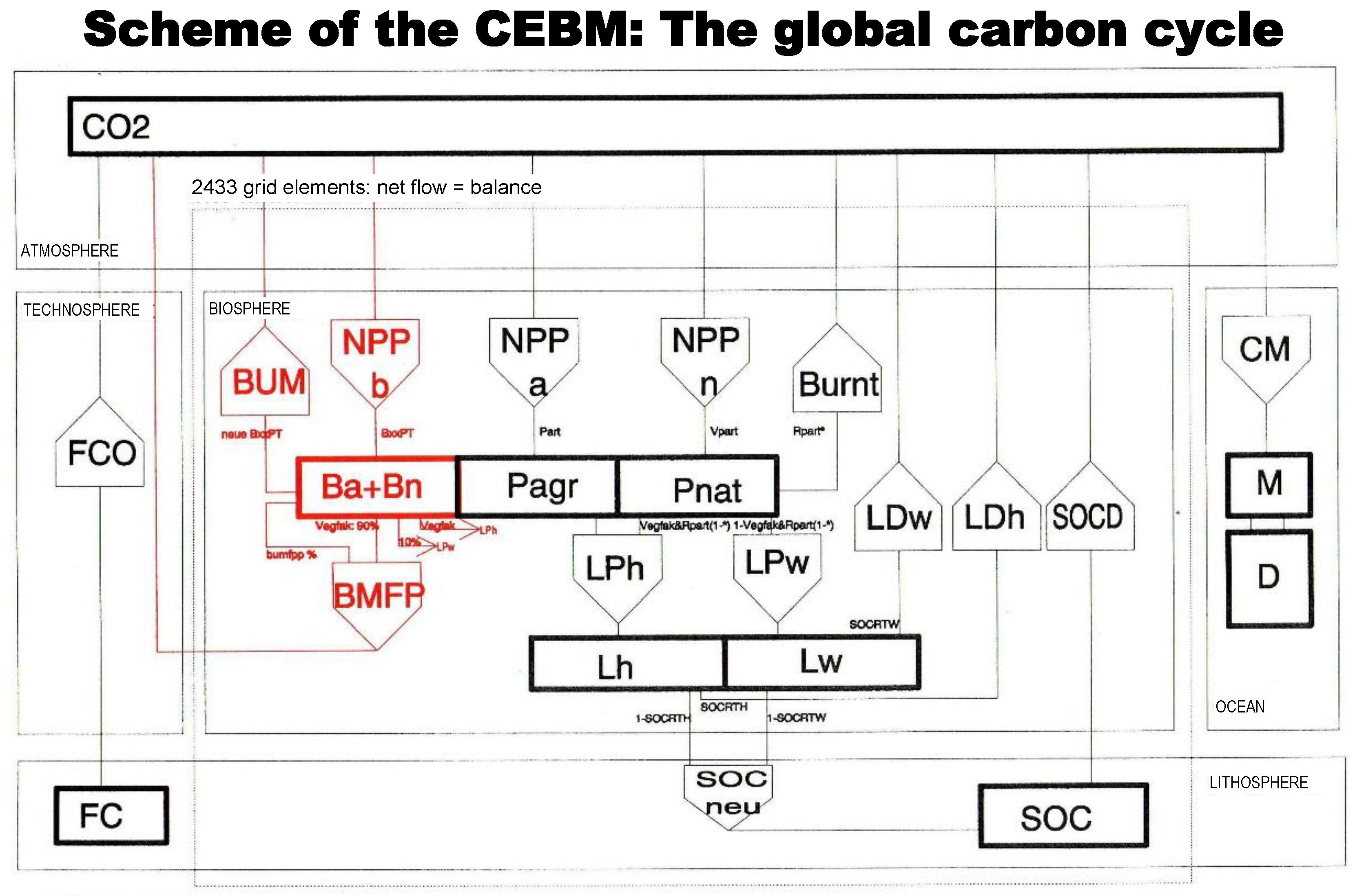
2.1. The Quantitative Tool: Combined Energy and Biosphere Model (CEBM)

This section explains the CEBM and presents the model structure with an overview of all carbon pools and flows.
The “Combined Energy and Biosphere Model” (CEBM) represents a global carbon cycle model and was created by the author based on the earlier Osnabrück Biosphere Model (OBM). The OBM had been developed by Prof. Gerd Esser in Osnabrück and Giessen, Germany [22,23,24,25,26], then refined at IIASA Laxenburg, Austria (where he handed over the OBM to the author for modification, which led to the CEBM), and later developed the OBM into the High Resolution Biosphere Model (HRBM) [27,28], again by G. Esser. The HRBM was included in several benchmarking exercises for global carbon cycle models [29,30,31] (and the author developed a land-use change module for it). The CEBM doubled the program size of the predecessor model OBM [32] (pp. 238–259), and it includes a tool for energy scenarios (Figure 9 in [32]). In its biospheric program section on worldwide 2433 grid elements, the CEBM allows the entire global carbon cycle to be calculated, including its main compartments of atmosphere, ocean, standing biomass, litter (fallen leaves and twigs) and soil organic carbon (SOC). The main carbon (C) flows (mediating between these carbon pools) are annual plant growth and plant decay depending on local temperature and precipitation levels [33] (p. 305). These C flows create a steady-state equilibrium as is typical for any living system [34]. CEBM model runs show that the global stability of the carbon cycle is determined by the relationship of magnitudes within the different existing fluxes. High sensitivity to outside disturbances occurs when these disturbances represent a large percentage of the flows in question [34,35,36,37,38,39,40,41].
This global model shows that the removal of biomass or residue from natural systems is likely to reduce soil carbon. This likelihood has been pointed out before (e.g., [41,42]), while [41] (p. 981, first para) assesses the CEBM definition of carbon pools (soil organic carbon and litter) to equate those definitions in the then most recent IPCC report.
A more direct description of how the annual carbon cycle is modelled on each of the 2433 grid elements worldwide (dotted line in Figure 1) starts out from the pool “atmospheric CO2” (labelled CO2, on top of Figure 1) and is directed as “Net Primary Productivity” NPP towards the standing phytomass (plant matter, P). As can be seen from the three parallel arrows, the CEBM distinguishes between natural areas, agricultural areas and areas dedicated to biomass energy, which add up to 100% of each or the geographical cells, amounting to some 250 km × 200 km. The phytomass P can degrade along two paths, namely to create either woody or herbaceous litter (typically, branches and leaves falling to the ground in autumn) and then follow microbial decomposition and return to the atmosphere—be it via the long-term buffer pool of “soil organic carbon” SOC. In the CEBM, instead of naturally decomposing, plant matter can also be combusted as biomass fuel (BMFP, red sector in Figure 1) and can replace the same heat value of traditional fossil fuels (FCO)—again being directed towards the atmosphere and thus closing the annual loop. Luckily, about 45% of global fossil emissions are absorbed by ocean waters (CM) in the mixed (M) or deep (D) water layers, thus preventing from a twice as fast increase in atmospheric CO2 concentration.
As a principal preliminary test for whether fundamental credibility is deserved, when inputting global annual fossil carbon emissions, the model reliably outputted atmospheric CO2 concentration as experimentally observed; namely through so-called (i) initialization runs and (ii) control runs [32] (pp. 262–265). (i) The initialization run means that all carbon pools in the model start out at a level of zero and are gradually filled by the annual carbon flows as defined through parametrization, in order to provide an equilibrated status of “only natural functions on the planet, without human interference” (Annex A3 in [32], similar to [38]). (ii) The control run means that from the historic starting year of 1860 (beginning of industrialization), the anthropogenic (fossil and deforestation) emissions begin to alter that equilibrium and successfully model the atmospheric CO2 concentration exactly (by a few ppm) as experimentally measured (Annex A4 in [32]). In a next step, the model used a defined fraction of every grid cell’s area for the production of biomass fuels which then could be used for replacing fossil fuels while keeping the calorific value of both fuel types identical.
By its detailed modelling of existing steady-state equilibria within the global carbon cycle (see Figure 1, depicted in detail through maps and time series in [33] (pp. 53–64+291–309), the CEBM is able to truly model biomass fuel usage, namely the net effect of the enhanced combustion of biomass. Such a dynamic viewpoint is not taken by a merely static calculation that only views two identical global carbon flows, namely “CO2 emitted by biomass fuel combustion” and “CO2 absorbed (i.e., sequestered) by biomass fuel growth” (symbolized in Figure 12 at left)—wherein these two carbon flows would simply add up to net zero. As this article shows, only a static view supports the idea of principal and theoretical carbon neutrality of biomass fuels, but a dynamic view tracing all single carbon flows realistically (Figure 12 at right) does not support the idea of principal carbon neutrality of biomass energy.
Before trusting the quantitative results of the model’s structure of flows and pools, and especially the effects of outside changes on this dynamic equilibrium, for several months the sensitivities of global carbon pools and fluxes were analysed in dialogue [43] and dozens of timelines and maps of these flows and pools were studied as a function of different scenarios for energy, emissions and deforestation (pp. 195–585 in [32]; a small selection is in Table A1) and compared with literature. It became apparent that disturbances in the global carbon cycle showed reasonable effects and known biogeochemical parameters such as soil organic carbon (SOC) are suitably generated as a function of thousands of model years [17,27,28]. Thus, the author trusted the model to provide suitable results also for future years. Numerous field studies had been taken into account by the authors of the predecessor models [22,23,24,25,26,27,28] when parametrizing the carbon flow. As shown in Figure 1, influx into the SOC pool stems from litter, i.e., both woody and herbaceous plant parts (Lh + Lw) that decompose annually, depending on the local climate. Flow out of the SOC pool is also governed by a heuristic formula (rightmost column in Appendix B) which was assessed multiple times by the author of the predecessor model [22,23,24,25,26,27,28].
The above section described the main pools and fluxes in the natural global carbon cycle and the anthropogenically disturbed carbon cycle.

2.2. Very Diverse Sensitivities: Annual CO2 Emissions, Deforestation and the Fertilizer Effect

This section offers several quantifications prior to the main research question of “carbon neutrality of biomass fuels” and focuses on the fertilizer effect (Section 2.2.1), deforestation (Section 2.2.2) and energy-related CO2 emissions (Section 2.2.3).
As a quick but reliable assessment of three often suggested hypotheses on how sensitive different assumptions are for the resulting atmospheric CO2 concentration, several CEBM model runs allowed the impact of (1) CO2 fertilization, (2) deforestation and (3) fossil CO2 emissions to be determined on the modelled level of atmospheric CO2 concentration for the year 2100.

2.2.1. The Fertilizer Effect

In earlier decades of climate protection, a frequent argument against the need for CO2 emission abatement was that “the entire globe’s biomass would absorb human fossil emissions anyhow”, namely by enhanced plant growth in an atmosphere with elevated CO2 concentration levels. The CEBM is able to refute such an argument (that actually had more of the character of an excuse), namely that the so-called “CO2 fertilizer effect” would offset fossil emissions (model benchmarking for its parametrization had been undertaken [40]). According to the formulaic implementation of existing and quantifiable knowledge about the so-called CO2 fertilization effect (i.e., plant growth in a given year is stronger with higher atmospheric CO2 concentration) on the growth of plants in the model, the impact of this effect on carbon sequestration is close to the error margin, hence almost undetectable [44]. (It can thus be concluded that a possible effect of more intense and frequent extreme weather events on the amount of annually growing biomass would be still more difficult to model at this stage—and is therefore left out from this model version). This is mentioned here because advocates of the coal industry in earlier decades claimed a strong offset of coal-related CO2 emissions by this fertilizer effect, and even produced a film “The Greening of Planet Earth” [45,46,47,48] (p. 283, footnote 166) in which the whole area of the Sahara Desert turned into green colour “thanks to emissions from coal fuels”. Such advertisements were led by strong economic interests and tried to misguide public opinion in earlier decades. A major underlying reason is that this effect pertains only to the annual turnover of carbon but clearly not to the standing biomass which remains roughly the same [32] (Figures 11, 17 and 21 therein), or to be exact, increases by 1–2% only within a range of low and high scenarios [33] (p. 307).

2.2.2. Deforestation

The target of this subsection is (i) to evaluate the effect of deforestation on atmospheric CO2 and (ii) to study and assess CEBM model behaviour after extensive land-use changes, with a view to planned biomass scenarios. For deforestation activities, the model includes a first quick emission (i.e., burning) followed by a longer, steady phase of emission (i.e., decomposition) [49]. A “reasonable” (or at least conceivable) variety of deforestation scenarios (defined by what is held plausible in current literature, based on an unpublished literature analysis performed by the author at IIASA) ranges from the preservation of 90% of global forests to their total annihilation by 2100—thus portraying even the theoretical maximum of diverse futures for deforestation. Model runs show that the resulting variability of atmospheric CO2 concentration amounts to a thirtieth of the variability due to diverse fossil scenarios [32] (Figure 42 therein). Hence, quantitative proof is evidence (once again) that fossil emissions are the key leverage for combating global warming by any suitable policy [33] (pp. 45–50, Figure 5.6 therein, pp. 291–310).

2.2.3. Energy-Related CO2 Emissions

While “preliminary energy scenarios” for the CEBM ranged from annual growth rates for CO2 emissions of −3% to +5% (with “+3%/a” representing a high scenario and “+1%/a” representing a moderate but still unsustainable scenario), these gross numbers do not yet reflect sufficiently well the underlying nation-by-nation techno-socio-economic dynamic patterns. In this CEBM program version, preference was given to the assessment of the impact of biomass scenarios, and therefore the energy scenarios were considered mainly as a background against which the net impact of biomass strategies is measured. In order to allow for a comparison with the scenarios proposed by IPCC AR5 [50], the scenario “+3%/a” is largely equivalent to AR5′s RCP8.5, often described as a “business-as-usual” scenario, and the scenario “+1%/a” is largely near (or a bit higher than) RCP4.5, which might be seen as a reduction scenario which, however, still proves insufficient for current 1.5 °C targets but might instead result in 3 °C warming after centuries. These two CEBM scenarios result from linear combinations of sub-scenarios for population, economic level, energy intensity (=E/GDP) and fuel mix and are provided in detail in [32] (formulae on pp. 104–106) and in [44] (pp. 119–129).
The main message of the above section is that the most essential impact on the global carbon cycle is energy-related CO2 followed by deforestation-related CO2 and then followed by the so-called greenhouse effect. This means that any political strategy should firstly address fossil energy and secondly deforestation while—thirdly—the so-called greenhouse effect can clearly never serve as an “excuse” that nature itself would be able to balance out human impacts on the carbon cycle.

3. Results

CEBM model runs are undertaken with various scenario assumptions in the style of a “what—if” logic and allow conclusions when comparing different scenarios. In order to give a first overview, the scenarios portrayed in Section 3 use as follows:
  • Underlying energy scenarios, namely, the following:
    One higher scenario corresponding to an annual CO2 emissions growth rate of +3%/a and
    One lower scenario corresponding to an annual CO2 emissions growth rate of +1%/a
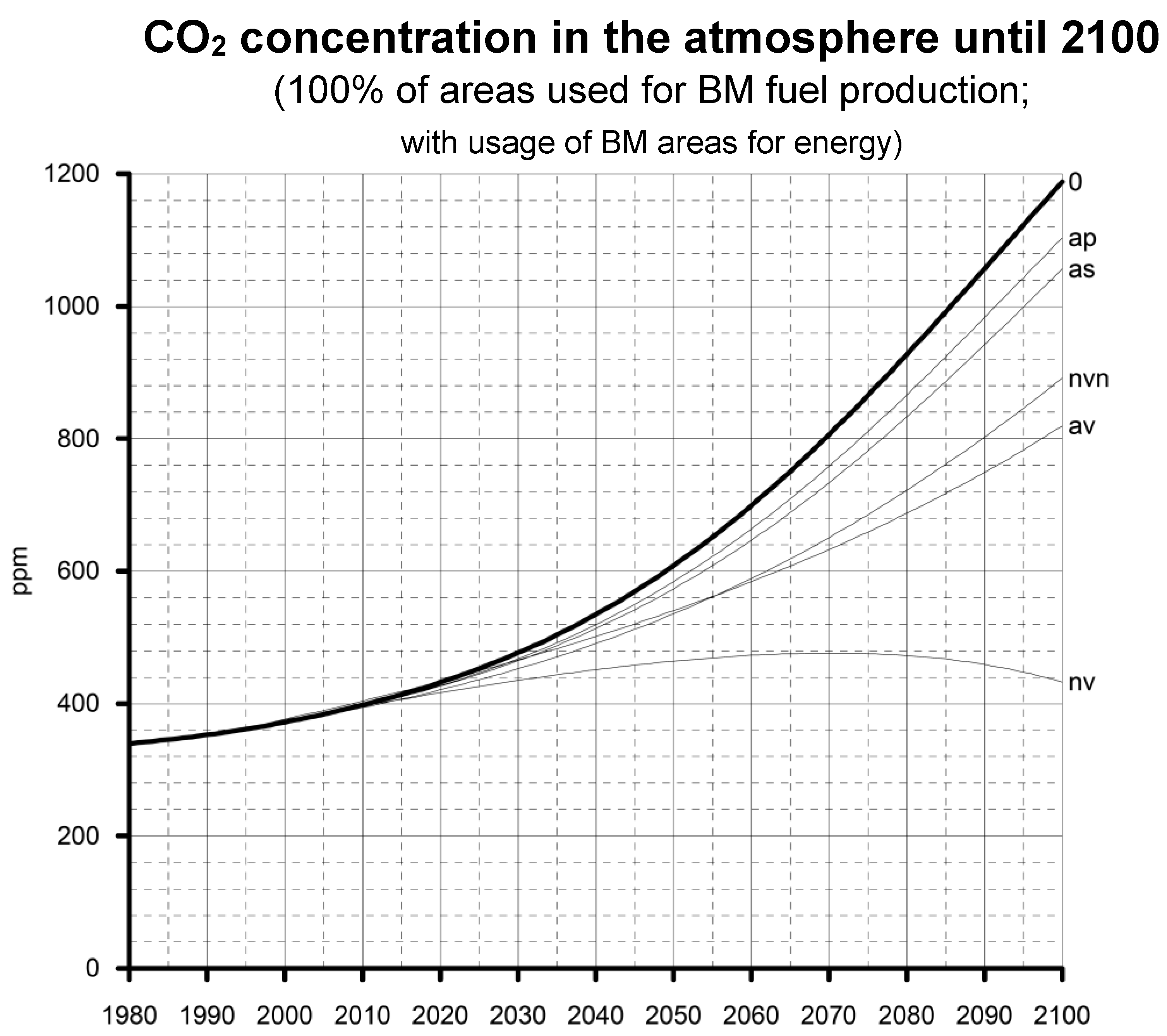
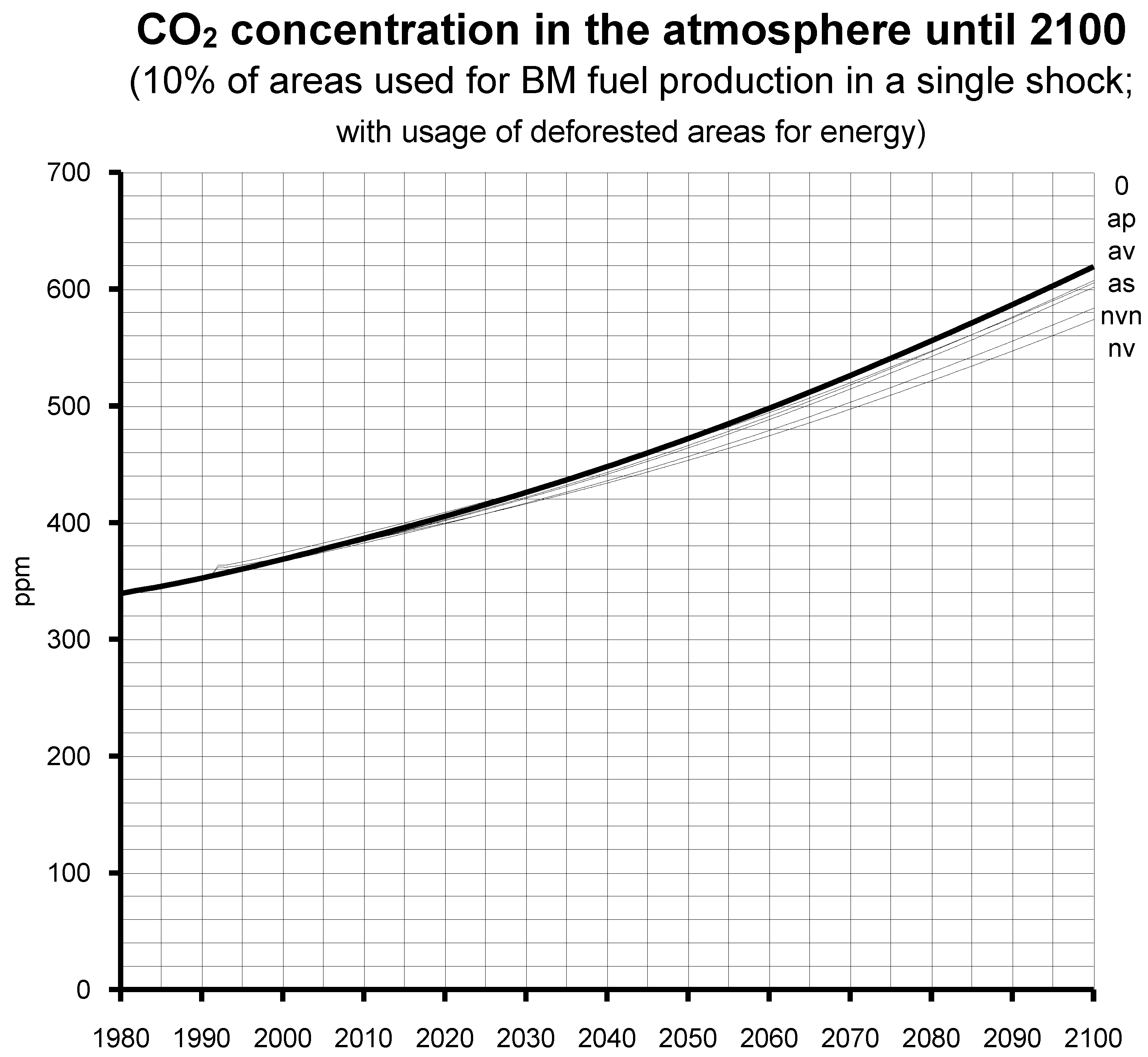
  • Upon which five types of scenarios for production types are applied, namely those described in Table 1, being ap, as, av, nv, nvn.

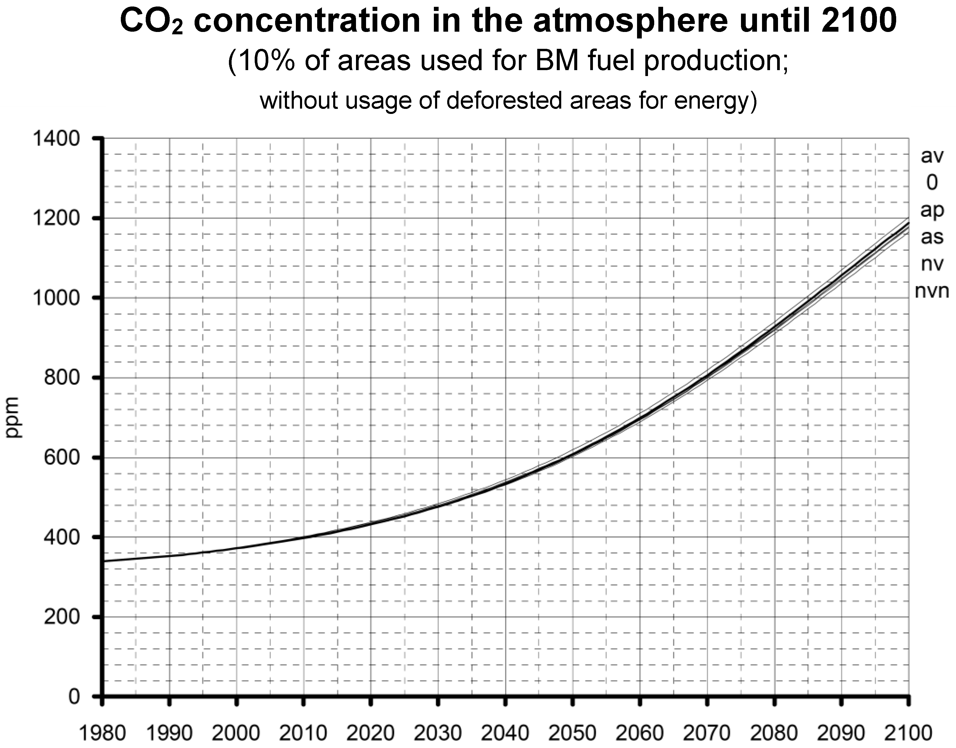
3.1. Scenarios on the Amount of Biomass Fuel Production Area
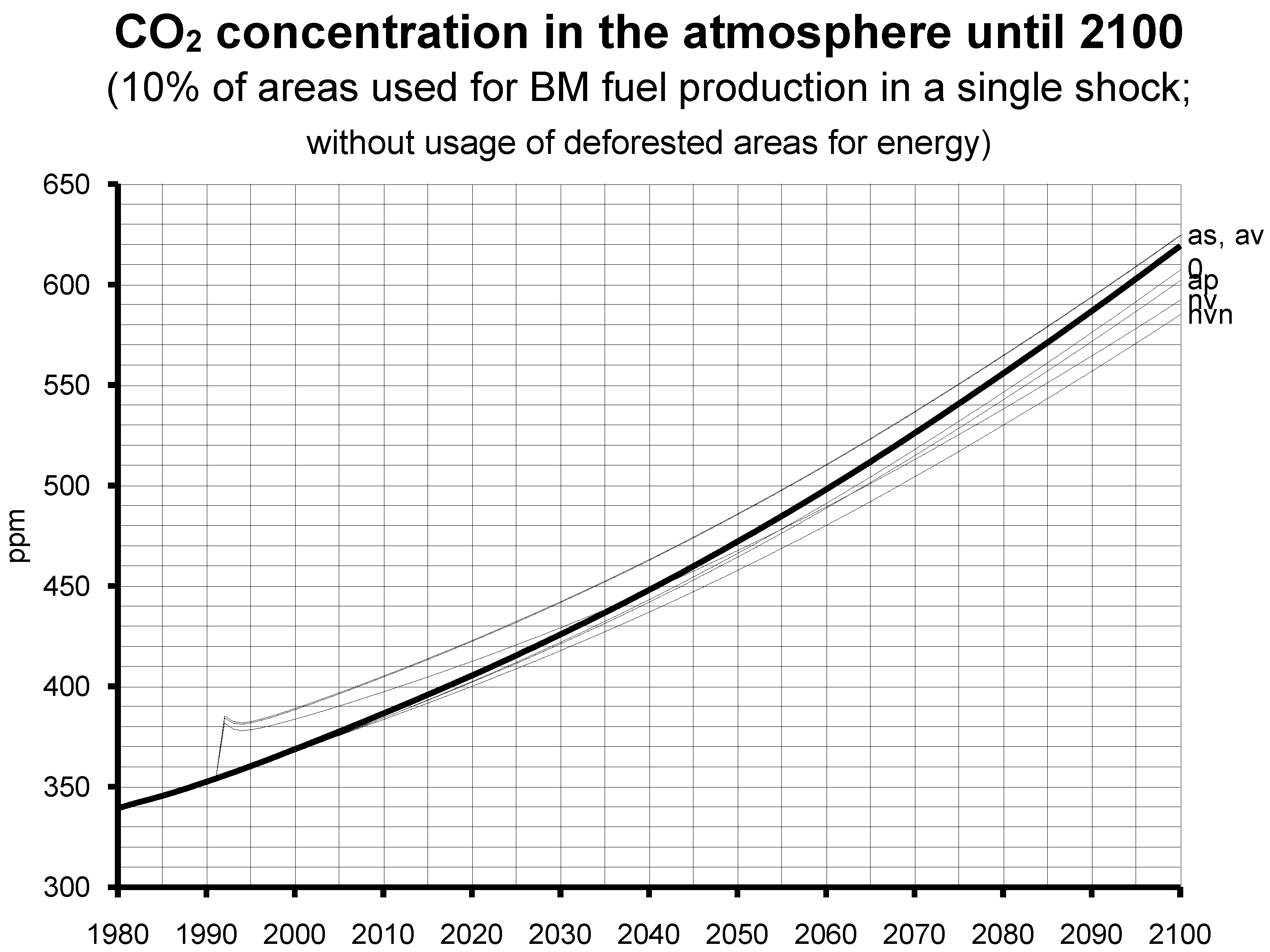
This section presents five modes of scenarios on how biomass energy may be grown and computes the results on the atmospheric CO2 concentration of these five biomass production types under varying frameworks.
In several sets of biomass (BM) energy scenarios (details for the five principal growth strategies are explained in Table 1), widely varying assumptions for the overall area dedicated to BM energy production were implemented, thus resulting in over 70 test runs of the CEBM. In general, the CEBM allocates each grid cell of land area to a certain percentage either for “natural” areas (e.g., forests, meadows) or for agricultural areas (with fields for food production), while both land-use types add up to 100% (this omission of urban areas might mean a small inconsistency but the final carbon pools and fluxes do not suffer from the deviation of a few percent). For the target of biomass energy growth, the CEBM can take a certain annual share of either natural or agricultural area and reallocate it to biomass production. One self-evident background is that humanity certainly needs areas of natural growth (to maintain biospheric cycles) and especially agriculturally used areas (for cereal etc. growth). Thus, it is evident that (in the CEBM) biomass can only grow if either natural or agricultural areas are diminished, because no large amounts of empty or barren land are available, except with unrealistically huge efforts for supplying water, humus and a suitably decent climate. When deliberating the extensive usage of areas for biomass energy production modelled in the below-mentioned scenarios, undesirable social conflicts will quickly arise—all the more because biomass energy has no great energy density and hence requires large areas.
Two main groups of biomass production scenarios included:
I
Every year, 0.1% of each grid cell’s (either natural or agricultural) area is dedicated to biomass energy production (Figure 2 and Figure 3), thus after a century resulting in 10% of the initial area being dedicated to BM fuel production and therefore still leaving sufficient space to the original usages of either natural or agricultural vegetation.
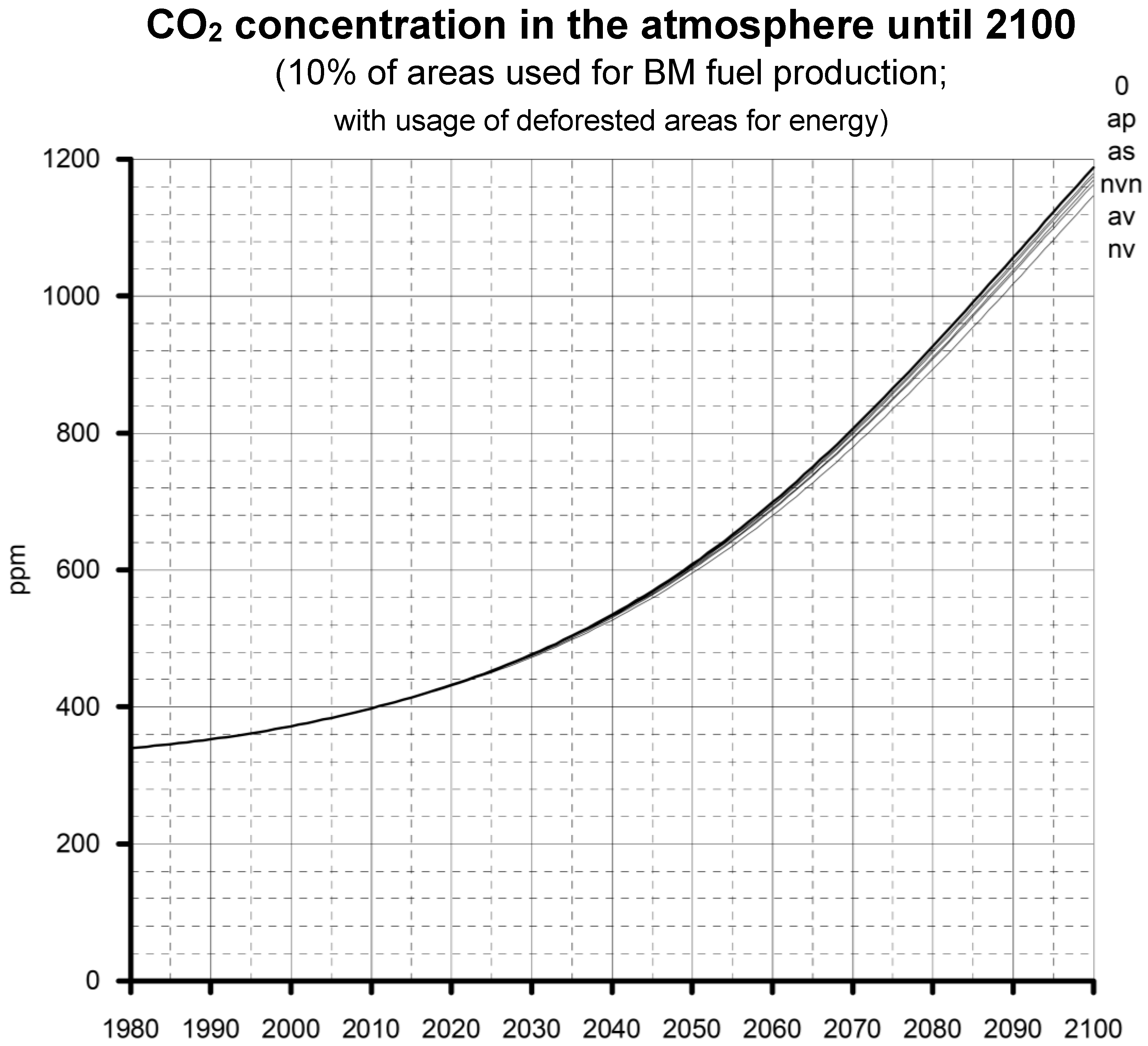
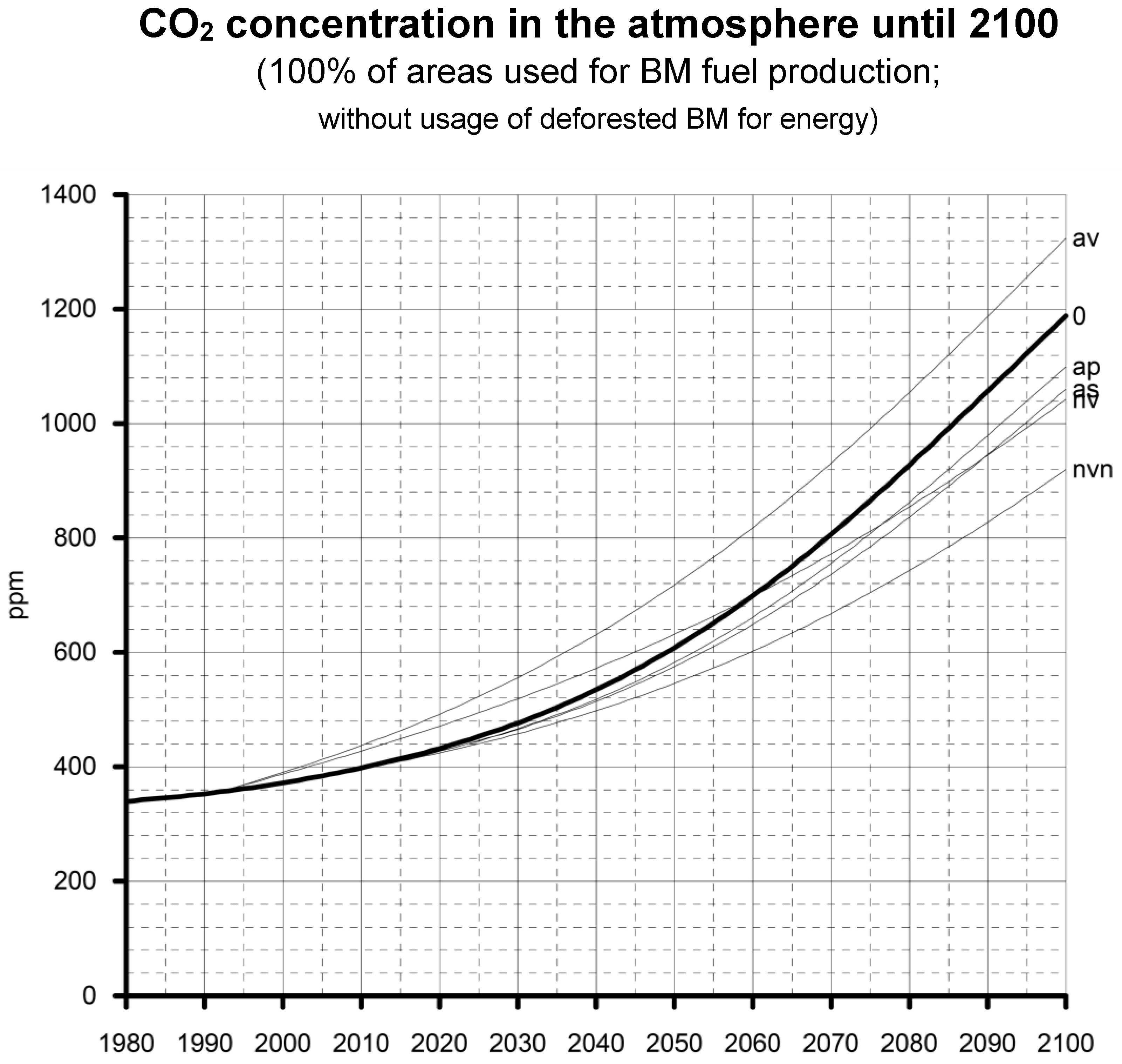
II
Every year, 1% of each grid cell’s (either natural or agricultural) area is dedicated to biomass energy production (see Figure 4 and Figure 5), thus after a century resulting in 100% of the initial area being dedicated to BM fuel production and therefore leaving no more sufficient space to the original usages of the earlier natural or agricultural vegetation. It is now already visible that in this group of scenarios the disturbing effects for the entire planet are way too strong to ever still be called “sustainable”. But, nevertheless, such scenarios are undertaken here as hypothetical and hence harmless thought experiments (Gedankenexperiment, in German language) in order to assess the global effects of biomass energy effects pushed to a theoretical maximum.
Figure 2. In a “+3%/a” CO2 emission growth scenario, when dedicating 0.1% of areas for biomass production, all five described types of biomass scenarios (without combustion of standing biomass on possibly deforested areas) show only a very small effect on the atmospheric CO2 concentration (from ~1160 to 1200 ppm in 2100). In the av scenario, even the concentration is higher than in the control scenario (labelled 0), due to uncontrolled deforestation emissions.
Energies 15 09619 g002
Figure 3. In a “+3%/a” CO2 emission growth scenario, when dedicating 0.1% of areas for biomass production, all five described types of biomass scenarios (with combustion of standing biomass on possibly deforested areas) show only a very small effect on the atmospheric CO2 concentration (from ~1140 to 1180 ppm in 2100).
Energies 15 09619 g003
It is striking that in the first group of scenarios (I), with less strong enforcement of areas dedicated to BM fuel production, the overall effect on the atmospheric CO2 concentration is highly marginal, as is visible in Figure 2 and Figure 3.
Therefore, it makes sense to subsequently look into the effects of massively enhanced BM strategies, namely gradually covering 100% of either natural or agricultural areas with BM for fuels until the end of a period of a century (second group of scenarios II, see in Figure 4 and Figure 5), leading to more marked effects on the overall output parameter of the CEBM, namely atmospheric CO2 concentration.
In the language of the CEBM, the expression “with or without usage of deforested areas for energy” means the following: in all areas coming under usage for energy production (be these former natural or former agricultural areas), a standing biomass exists. This plant matter must be dealt with when introducing a new allocation for these areas. In principle, the biomass standing there can either be combusted and the resulting energy used to replace fossil fuels (in the same way as the future-produced biomass fuels replace fossil energies) or it can be combusted without such use for the production of energy. The latter choice would actually amount to deforestation through burning and thus be highly unsatisfying. The latter option “without energetic use of biomass from re-dedicated areas” therefore shows often extremely high CO2 emissions which of course directly counteract the initial target of biomass cultivation, namely hindering CO2 emissions. Given that choosing between these two principal options most strikingly influences the final result, in all Figures a clear distinction is made between the two choices.
Figure 4. In a “+3%/a” CO2 emission growth scenario, when dedicating 1% of areas for biomass production, all five described types of biomass scenarios (without combustion of standing biomass on possibly deforested areas) show considerable effect on atmospheric CO2 concentration (from ~920 to 1320 ppm in 2100). In the av scenario, the concentration is even higher than in the control scenario (labelled 0), due to uncontrolled deforestation emissions.
Energies 15 09619 g004
Figure 5. In a “+3%/a” CO2 emission growth scenario, when dedicating 1% of areas for biomass production, all five described types of biomass scenarios (with combustion of standing biomass on possibly deforested areas) show a high to extremely high effect on the atmospheric CO2 concentration (from ~420 to 1200 ppm in 2100)—but the downside is that the globe would be fully deprived of either natural or agricultural vegetation and hence uninhabitable.
Energies 15 09619 g005
From the above four figures, the main message can be for both main groups of biomass production scenarios as follows:
I
=> a net effect on the global atmospheric CO2 concentration is almost not visible, hence such a “soft” scenario mode helps too little in mastering the initial research question, namely fighting global warming.
II
=> while considerable mitigation of the greenhouse effect is achieved, the main message is that engendered disturbing effects on the entire planet are way too strong to ever still be called “sustainable” in any respect. These disturbing effects include the following: huge damage to existing land-use change patterns, destruction of the entire (either agricultural or natural) vegetation cover for the sake of energy production, and disturbed ecological and economical patterns on all levels. In such scenarios, the globe would be completely deprived of its natural material cycles, and thus planetary biochemistry would be overturned with additional damage to the climate (that was intended to be saved in the first place).
Hence, the above four modelling scenarios teach as follows: either the mitigating effect of biomass energy is very small on the global greenhouse effect, or if the mitigating effect is large enough, the limits of sustainability are not kept.

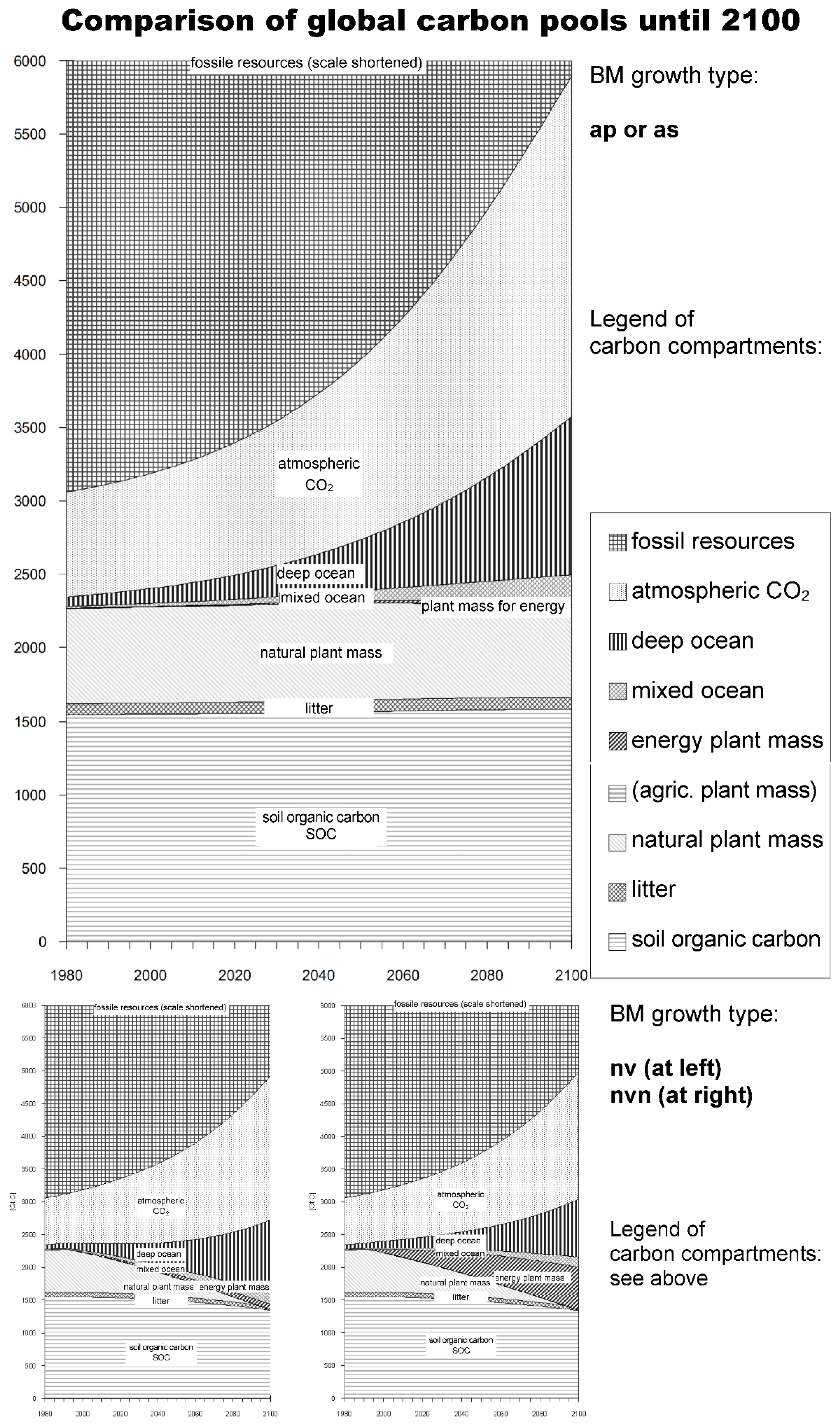
3.2. Shifts in Global Carbon Pools and Fluxes Resulting from Biomass Growth Scenarios

The above-mentioned scenarios produce long-term shifts within the global carbon pools as shown in the sections of Figure 6, and within the scheme of global carbon fluxes as shown in Figure 7.
Figure 6 provides a synopsis of all involved carbon pools as a global sum. It therefore becomes visible that the depletion of the fossil pool by energy-related fossil emissions leads to a carbon shift into the following two other reservoirs: the atmosphere and the ocean. It might be a helpful rule of thumb for quick reference that half of the fossil emissions end up in these two compartments. When focusing on the difference between the three biomass growth types, the comparison shows that using agricultural areas (image above, type ap or as) leads to no visible changes in plant mass, but usage of the globe’s natural areas leads to the complete replacement of natural plant mass by plant mass devoted to energy production—and this article discusses several times how unrealistic and how extremely unsustainable such a strategy is.

3.3. Results from the Scenarios on Biomass Energy Growth

This section presents conclusions from the above results regarding the global potential of biomass energy carriers.
One collateral result of the above-mentioned scenarios on five strategies of biomass growth (see Table 1) is the global potential for biomass fuels, i.e., the capability of the biosphere to produce biomass that can be combusted [33] (pp. 61–64). It is emphasized that all scenarios within the CEBM assume that only the amount of annually growing biomass is used for combustion but not the amount of standing biomass (=standing plant matter = P in Figure 1 and Figure 7 = phytomass as such), in order to implement at least one aspect of sustainability in very general terms. Thus, the arrow indicating biomass fuel production (BMFP, at the extreme left in Figure 7) represents a flux that deliberately branches off a considerable share of the naturally existing flow named NPP (= net primary productivity = annual growth of plants).
In this sense, we now contemplate the theoretical maximum fuel potential (of the highest yielding of all five biomass growth strategies, which is clearly nvn). As a quick orientation, the calorific value (when only viewing the value of annually grown wood) is of an order of magnitude that roughly corresponds to current global energy consumption. The connected reduction effect on atmospheric CO2 concentration is about 300 ppm (see Figure 4 at the right)
However, as in the course of the remaining century the overall global energy demand will have increased considerably, this potential will appear as very modest—especially given the huge effort needed to exhaust this potential through large-scale re-allocation of land use.
Such a limited biospheric potential of the energy carrier biomass assumes (realistically) a yield for plant growth identical to the present yields from either natural or agricultural biomass on each of the 2433 grid elements across the planet. It seems unrealistic to just dream of drastically higher plant matter yields because tremendous efforts for irrigation and soil improvement would be necessary across wide swathes of the earth.
As mentioned, when limiting oneself to more moderate biomass strategies (Figure 2 and Figure 3), the resulting effect on the atmospheric CO2 concentration (which is the final output parameter of the CEBM), amounts to only around 20 ppm (see Figure 2 at right) which can be considered to be non-rewarding when comparing with the huge efforts needed for any worldwide biomass energy strategy.
Summing up this section, there are only the following two possibilities: either the imaginary global biomass-centred energy supply system supplies such large amounts of biomass fuel that a greenhouse reduction effect is perceptible and thus causes disturbances in the carbon cycle of the biosphere (removal of plants, soil depletion); or one takes into account the limited load-bearing capacity of the plant cover and has to do without the originally desired abatement of the greenhouse effect.
The above section offered four groups of scenarios that allow us the assessment of (i) how the main shifts within the global carbon cycle occur and (ii) how a theoretical maximum of the global biospheric biomass energy potential is quantifiable.

3.4. Scenarios with Lower Increase Rates of Global CO2 Emissions

This section presents modified model runs (as compared with Section 3.1) in order to assess less radical impacts (namely, only a tenth) on the planet’s biosphere.
All the scenarios examined so far were against the background of a consistently strong increase in fossil energy-related CO2 emissions during the 21st century of +3% per year (“+3%/a”), which might prove very realistic given earlier and present trends [51,52,53]. In this situation, analogous biomass scenarios are tried out with a lower CO2 emissions overall trend, namely at +1%/a. At the same time, these scenarios serve to evaluate another effect of biomass energy strategies that until now was hidden within the multitude of different reactions of the global carbon cycle’s dynamic equilibrium as follows: what does the re-utilization of formerly natural or agricultural areas produce in terms of net atmospheric CO2 concentration? To detect such an effect, the assumption was made that within one single year (in this case, hypothetically in 1991), 10% of the entire (either natural or agricultural) area in every grid cell is used for the production of biomass fuels (according to the five strategies described in Table 1). Figure 8 and Figure 9 show the result, with and without usage of deforested areas for energy, respectively.
The above section portrays the impacts of a less-than-maximum biomass energy strategy worldwide and shows how limited its positive effect on the resulting CO2 concentration is.

3.5. Summing up the Effects of Biomass Strategies on the Global Carbon Cycle as Result of the CEBM

This section presents the overall lessons learned from all the above model runs, grouped into eight main items.
Based on the above calculations, the most important effects of the energetic use of biomass on the global carbon cycle include the following:
(1)
Fossil CO2 emissions decrease (to a slightly lesser degree than the extent to which emissions from biomass fuels are added in exchange, the reason being the weaker calorific value of wood as compared to current fossil fuel mix of coal, oil and gas),
(2)
In some scenario types, the global total phytomass becomes decisively decreased (because naturally standing forests accumulate more carbon per area than dedicated biomass fuel plantations of whichever of the five strategies mentioned above)
(3)
In all scenario types, the carbon flow through the litter compartment (in Figure 1 and Figure 7) decreases (as a result of the “BM fuels” (flux BMFP in Figure 1 and Figure 7) being carried away from the areas) and the inflow into the soil carbon compartment (SOC in Figure 1 and Figure 7) also decreases as a consequence. This SOC pool loses C as a direct consequence of biomass fuel usage; in some cases, considerably, which is ultimately due to the removal of material from the steady state of the natural global carbon cycle that has reached a planetary steady-state equilibrium after thousands of years (computationally, reaching of this equilibrium is shown [31] (pp. 262–263)). Over the decades, this effect produces a very considerable net depletion of soil organic carbon (i.e., of humus) globally.
(4)
The amount of carbon released as a result of the possible rededication of natural areas to those with a lower forest density must be taken into account; their emission into the atmosphere is undesirable, and very astonishingly is of strikingly high magnitude. Thus the “rededication emissions” (BUM in in Figure 1—meaning in German Biomasse-Umwidmung, i.e., re-allocation of areas from other dedications (a or n) to biomass production areas) which are equivalent and analogous to deforestation emissions, are likely to represent the main effect of biomass strategies, even if this was very unexpected to the author before performing the present study. Readers in the year 2023 are well aware of striking photos from palm oil plantations in the global South that replaced enormously rich and densely forested primordial areas [54,55,56,57,58,59].
(5)
A noticeable relief with regard to the increase in atmospheric CO2 content can be detected in the model results, but it approaches marginal values if the theoretical potential for energetic biomass use is not exhausted.
(6)
The effects on the global ecosystem will in many cases be more than considerable.
(7)
However, a model result of the CEBM is that the energetic use of biomass contributes to the slowing down of the increase in atmospheric CO2 concentration.
(8)
An assessment beyond the area of the carbon cycle is not possible by the CEBM because it perceives merely carbon fluxes, not fluxes of other chemical substances such as oxygen, nitrogen, minerals or any nutrients—or soil quality at large—or any wider biospheric magnitudes such as biodiversity of economic parameters. Therefore, other deliberations certainly must complement the CEBM results. It can be expected that the assessment of the value of biomass strategies will then be seen in a still much more critical light.
The further weighting of all relevant effects has to take interdisciplinary aspects into account.
This section portrayed eight key impacts of extensive biomass energy use and highlighted (possibly surprisingly) that the largest effect should be expected from standing biomass prior to plantations.

3.6. CEBM Model Runs to Evaluate the Overall Carbon Neutrality of Biomass Energy

This section presents and interprets specific comparisons of CEBM model runs that serve to assess the degree to which biomass can be considered principally carbon neutral.
More quantitative conclusions on the degree of carbon neutrality (or its principal non-neutrality, as suggested in Item 3 above), can be drawn from comparisons of several more CEBM model runs that are pictured in Figure 11 and Table 2.
As an envelope to these additional scenarios, a “business as usual” scenario (full line, above, yielding 1190 ppm until 2100 and thus largely identical to a “+3%/a” scenario) and a climate-compatible “reduction target” scenario (dashed line, below, yielding 435 ppm until 2100 and thus largely identical to a “−1%/a” scenario) are added. These two scenarios might describe the range of likely future developments across the majority of socio-political assumptions triggering resulting global CO2 emissions. Moreover, the “basic” scenario (squared points, centre, yielding 640 ppm until 2100, largely similar to a “+1%/a” scenario) provides the basis of comparison for the following two scenarios: biomass and low emission.
The deliberation is as follows:
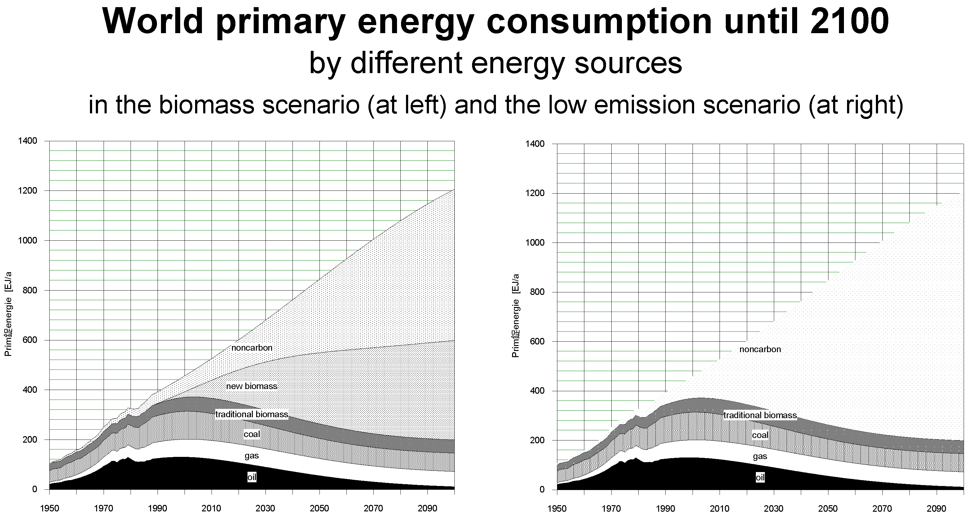
  • In a base case, energy demand (derived in [32] (Chapter 8)) can be covered until 2100 by a strongly reduced percentage of fossil fuels and by a courageously assumed (roughly) half of sustainable non-carbon sources such as solar and wind (nuclear is explicitly not intended!) and the remainder of energy demand is covered by “biomass”—which the core interest of the present study. This is called the “biomass scenario”, depicted at left in Figure 10.
  • If the “biomass” share of the above “biomass scenario” is covered by non-carbon energy as well, then the world can satisfy the same energy demand with different energy carriers.
Figure 10. How the assumed (moderate) energy demand until 2100 is covered by single energy carriers. While overall energy supply is identical in both cases, the energy demand covered by biomass at left is covered by non-carbon sources at right—thus allowing C-neutrality to be assessed.
Energies 15 09619 g010
Figure 11. Compilation of several scenarios that allow the evaluation of whether biomass energy is systematically carbon neutral, or the extent to which this carbon neutrality is smaller than anticipated.
Energies 15 09619 g011
When comparing the two above-mentioned scenarios, the difference in resulting atmospheric CO2 concentrations should be zero in cases where biomass energy is truly carbon neutral, because it would make no difference to use non-carbon sources (such as solar and wind) or “carbon-neutral biomass”.
However, the CEBM model results show a considerable difference as follows: the reduction achieved in atmospheric CO2 concentration from the base scenario (squared points in Figure 11) to the biomass scenario (full diamonds in Figure 11) is not as great as the reduction achieved from the base scenario to the low-emission scenario (empty diamonds in Figure 11). The remaining difference is identical to the amount by which the energetic use of biomass is not completely CO2-neutral.
It is easy to read graphically that after taking into account the net effect of the complex carbon cycle processes within the biosphere (as modelled in Figure 1) in an overall view, biomass fuels are actually CO2-neutral only to about half of the theoretically expected (and desired) extent. This is an astonishing result and can be easily understood by the depletion of the worldwide soil organic carbon pool, due to the redirection of considerable amounts of wood away from their “natural destiny” of being decomposed into litter and then into SOC (humus). Overall, biomass production areas will therefore considerably deplete in humus, given the fact that the decomposition of humus by microorganisms (flux SOCD in Figure 1) continues as usual by the unchanged activity of microorganisms in the soil. Those microorganisms are unaware of human redirection of C flows.
To the extent that the CEBM correctly models these aspects of reality, and to the degree it is a suitable computational model, this result of “biomass is only half as carbon neutral as previously hoped” is to be regarded as one of the main results of the entire CEBM modelling endeavour and strongly calls into question the naming of biomass as a “carbon-neutral energy source” in the framework of international climate protection strategies and of accounting rules for national emissions.
It is highlighted that this “halved carbon neutrality” is true even if transport, conversion, losses and other connected fossil emissions are not taken into account. Even if (in a highly idealized image) these preparatory and secondary emissions are later to be covered by biomass energy sources on their turn, it will not heal the principal non-neutrality of biomass from a purely theoretical standpoint, i.e., when viewing only carbon flows and when limiting biomass energy to directly combustible wood matter (which is not true anyhow because of the need to convert BM into liquid fuels for the sectors of transport, e.g., [60,61,62,63,64,65,66]). Additionally, all effects and cycles of biomass growth and harvest take place over very long periods of time, as is typical for any deliberation within forestry.
The above section combined three specific scenarios and allowed the following conclusion to be drawn: on a principal level, biomass energy is less carbon neutral than is widely assumed.

3.7. Effects on Rules for Emission Accounting for Biomass Energy and Biomass Sinks

This section presents the consequences of the above assessments on the rules for carbon accounting.
Each country was and is obliged to report its emissions annually, based on emission reporting guidelines in force at a given time, defined by the IPCC [67]—while carbon accounting of the biosphere still encounters many principal difficulties [68,69,70,71,72,73,74,75,76,77,78,79,80,81,82,83,84]. As described on page 6 of the (unpublished) detailed version of the Austrian Air Emission Inventory 1980–1996 [85], the overall reporting activity should differentiate better into the single carbon flows involved in biomass energy, and not be restricted to simple “carbon neutrality”. This might have been improved in the meantime.
In light of the Austrian situation, during the past decades, carbon sinks have always accounted for highly negative values with “land use change and forestry” of the carbon balance [86]. According to the authors Jonas and Schidler, the following three different factors have contributed to the major fluxes from the atmosphere into the biosphere:
  • Net increase of areas covered with forests in Austria
  • Increase of net stock density per unit area
  • Increase of average age of forest stands because trees are harvested on average at a later stage.
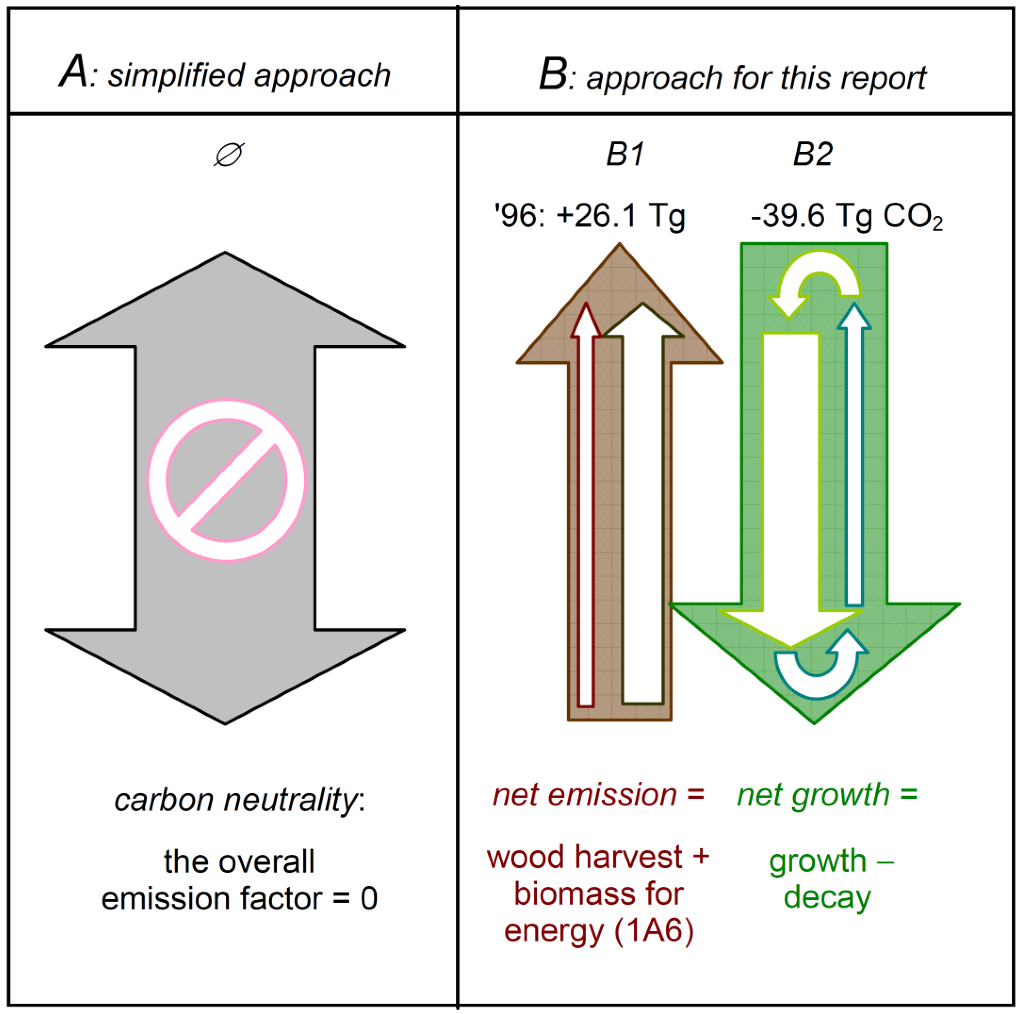
In principle, there are two different approaches for accounting for carbon fluxes with regard to harvesting and combusting biomass (see Figure 12). However, care must be taken in order not to confuse the two concepts by eventually omitting one partner of two corresponding flows.
A.
Biomass is regarded as a carbon neutral fuel. In a sustainable production system, the CO2 emissions occurring during biomass energy usage and biomass growth are considered to be equal, which is approximately the case in the medium term (grey double arrow). Here, the CO2 emission factor equals zero. This simplified view is sufficiently exact in some cases and is reflected in the national total of the present report.
B.
In this more elaborate concept both carbon fluxes (net emission minus net growth) are represented (two arrows in the sketch). This approach enables possible non-nil net effects to be accounted for, due to (i) import or export of biomass fuels or (ii) net increase or depletion of carbon on the territory of a country as a result of various biogenic or other factors. Here the CO2 emission factor of biomass is equal to the carbon content of the wood but a corresponding arrow in the above sketch represents net tree growth for one year. In this approach, the level of differentiation corresponds to this concept (see pp. 6–7 in [85]).
It can be easily imagined that the choice of the accounting method creates considerable differences regarding the following
  • The performance of entire nations regarding climate change to date
  • Every nation’s decision for future climate policies.
The above section supported the conceptual step from merely assuming carbon neutrality towards neatly differentiating into all single flows when it comes to national carbon accounting.

4. Discussion

4.1. On the Notion of the Overall Carbon Neutrality of Biomass Energy

This section presents the discussion of CEBM results regarding the carbon neutrality of biomass energy.
The above result can be explained as follows: As already mentioned, the decade-long extraction of plant material from an ecosystem leads, according to the results of the CEBM, to a depletion in the soil carbon reservoir (SOC, Figure 1 and Figure 7). In the end, these emissions also follow the path of all anthropogenic emissions, as do deforestation emissions and fossil CO2 emission as follows: they are mainly distributed across the atmosphere and the ocean. Consideration of the quantity of those “net CO2 emissions from global soils” shows that (depending on the model used), this effect amounts to about half of the amount of energy saved (still being dependent on to the exact type of biomass growth strategy (here nvn)). These “net emissions from the soil” result from the fact that the flow from this pool (SOCD) remains the same due to the almost constant degradation activity of the microorganisms, but the current flowing into the soil carbon reservoir (SOCneu) drops by an amount equivalent to the removal of biomass fuels. The latter can no longer take their “natural” route “existing litter => soil organic carbon” (see Figure 7).
Overall, intensive energetic biomass production represents a large-scale diversion of global carbon flows, which influences the stable flow equilibrium between previously largely untouched carbon reservoirs. These streams of carbon are used by humans to generate energy and, according to the model results, are therefore no longer available to nature for sufficient humus (SOC) formation. In this context, it should be pointed out once again that the exact extent of this soil carbon depletion effect depends mathematically on the formula for its degradation. This formula was recognised in [32] as empirical or even heuristic and possibly might be not exactly applicable to every spot of the globe. In general, it may well be that the modelling results of the CEBM do not exactly apply numerically; but with the current state of knowledge, the fact remains that such a carbon depletion effect nevertheless occurs, and that its scope is in all probability not negligible in the long term. The result found here seems to have a higher degree of likelihood with regard to its actual occurrence, but a lower degree of likelihood with regard to its quantitative extent.
It should be emphasised again that in the scenarios mentioned, almost worldwide use of natural woody plant growth for combustion was assumed. In order to circumvent the mentioned effect of the biosphere’s net CO2 emission, one could come up with the suggestion to use biomass for energy to a lesser extent. Such scenarios would influence the earth’s ecosystem much less, but would show only a very marginal contribution to the containment of the increase in atmospheric CO2 concentration (see Figure 8 and Figure 9).
It is of course possible to use other types of growth than “forestry” (nvn) from the five cultivation types mentioned in Table 1. However, the following two things have to be considered: On the one hand, the “nvn” (forestry) method is a method in which the biomass originally existing at a location can also be left untouched during the phase of fuel production (no land conversion emissions are possible); on the other hand, the other scenario types providing a significantly lower potential for fuel generation. This means that the global greenhouse reduction potential of other cultivation types (av, as, nv, ap) would be even lower.
It is mentioned here that the main result, namely, that harvesting biofuels is likely to reduce soil carbon, is corroborated independently by models created after the CEBM, including the Graz-Oakridge Carbon Assessment Model GORCAM [17,87,88,89,90] created by Bernhard Schlamadinger, with whom the author engaged in detailed discussions.
The above section positioned the CEBM results within a wider frame of other similar models assessing carbon neutrality.

4.2. Comparison of CEBM Results with Literature

This section presents a detailed comparison of CEBM’s results on the question of carbon neutrality with results from the scientific literature, with a focus on recent literature.
At first, this section provides evidence that the CEBM and its above-mentioned results conform with current knowledge of the global carbon cycle, and are backed by a wide range of models.
As one recent analysis [41] (p. 981, second para) states, “cycling of carbon is inherently linked with cycling of nutrients, particularly nitrogen”, and therefore author G. Esser [22,23,24,25,26,27,28] already strived to combine carbon cycle models with nitrogen cycle models early on. Evidently, it is crucial to correctly parametrize both influxes into and outfluxes from soil organic carbon (SOC) [41] (p. 981, third para) as a function of local temperature and precipitation, because in a cool temperate climates SOC accumulates over many thousands of years; whereas it does not in warm, wet or desert climates. Quantitatively, these net effects were double-checked by “initial runs” [32] (pp. 262–263) before applying the CEBM at all, and yielded the well-known geographical pattern for SOC [32] (pp. 334–336). The clay content mentioned in [41] (p. 981, fourth para) literature analysis and resulting soil quality are parametrized in the CEBM by an aggregate “soil factor” [32] (p. 307). The “different turnover times” for SOC mentioned in [41] (p. 981, fifth para) are parametrized by the overall CEBM formula for SOCD and LD [32] (pp. 310–312), see Table A1.
Different carbon cycle dynamics on soils with agricultural or natural vegetation ([44] (p. 982)) are mainly governed by distinct decay factors for herbaceous (applied to agriculture) and woody biomass (both of them being applied to natural vegetation), see [32] (pp. 310–311, combined with 313–318) and Table A1. The protracted effect of decomposition of deforested biomass is well mirrored by the functions governing deforestation emissions. The CEBM, in order to mirror the diversity of impacts of biomass usage for energy [41] (p. 986) had introduced the five biomass production types as defined in Table 1 and traced changes in plant stock density according to these types and their different woody/herbaceous ratio and stand age [32] (pp. 308–309+325–326). The GORCAM model [17] mentioned in [41] (p. 990) was developed at the same institute where the present author—who actually introduced GORCAM’s author to carbon modelling—worked; and therefore no conceptual rift between CEBM and GORCAM can be expected, except that GORCAM apparently does not describe the entire globe (as CEBM does) but only a fictive unit of soil area. The “net CO2/GHG balance” in [41] (p. 992, 2nd para) was computed by the CEBM for the entire globe [32] (pp. 308–309+319–324) and is available in the CEBM for each of the five biomass energy production types as a time series [32] (Chapter 7.2.2 on p. 106).
Moreover, also the conclusions of the FullCAM model proposed by Cowie et al. [41] (p. 997, lines 4–7) fully equate and endorse the CEBM conclusions presented here as follows: “There is a risk of depletion of soil carbon stocks in biomass production systems, because a higher proportion of the organic matter and nutrients are removed from the site compared with conventional grain and timber production systems. Environmental and management factors will govern the magnitude and direction of change”. However, ref. [41] (p. 997, line 27) assesses that soil carbon loss “is negligible in comparison with the greenhouse mitigation benefit of avoided fossil fuel emissions”. That is a different order of magnitude than the assessment by CEBM which, however, envisaged a period of one century for the effect to develop during gradually extended biomass energy use, which appears to be realistic and suitable to the author.
Another important (meta-analytical) study by Achat et al. [42] (p. 1) speaks about this same “carbon transfer for soil to atmosphere partly neutralizing the role of a carbon sink played by forest soils”. This means a more considerable compromising of BM carbon neutrality, as is stated in the present article. This meta-analysis, collected from 238 peer-reviewed publications, “reports a global assessment of the consequences of different management practices on soil organic carbon storage in forests” [42] (pp. 3–4+8) and offers an average SOC loss of −38% for “combined conventional and intensive harvest” of biomass—which is a huge effect indeed, given that the SOC pool amounts to four times the amount of the carbon pools in the atmosphere or in standing plant matter. Even if that analysis [42] (p. 8) assesses the change in only one carbon compartment (SOC), these results can be seen as being in harmony with those of the present study.
On the other side, the article by Schulze et al. [91] corroborates this article’s findings by stating the following: “We argue that such an increase in biomass harvest would result in younger forests, lower biomass pools, depleted soil nutrient stocks and a loss of other ecosystem functions. The proposed strategy is likely to miss its main objective, i.e., to reduce greenhouse gas (GHG) emissions, because it would result in a reduction of biomass pools that may take decades to centuries to be paid back by fossil fuel substitution, if paid back at all. Eventually, depleted soil fertility will make the production unsustainable and require fertilization, which in turn increases GHG emissions due to N2O emissions. Hence, large-scale production of bioenergy from forest biomass is neither sustainable nor GHG neutral”. In the same direction, ref. [92] diagnoses a “temporal imbalance” between the points in time of growth and harvest, thus hampering the desired neutrality at least as a quick relief to within a few decades, but necessitating non-negligible ‘payback’ or ‘repayment times’ (p. 375). In the same vein, ref. [93] (p. 196) calls for an “analysis of forest carbon dynamics” and assesses the following: “In summary, it is important to accurately assess the time required to achieve net emission reductions from substituting forest bioenergy for fossil fuels, as well as the possible increases in emissions before this time, and the emission reductions thereafter. Depending on the wood biomass sources, wood bioenergy can have immediate net emission reduction, or requires decades or more than a century to obtain the net reduction of emissions”.
The definition of the “displacement factors” (DFs, which relate the emission reduction to the carbon mass contained in the wood used) by Leturcq [18] turns out to be helpful for assessing the overall degree of how helpful a biomass energy strategy is. This author stresses that “energy substitution has an immediate adverse greenhouse effect since the emission factor of wood is higher than that of any other fuel” [18] (p. 7). Additionally, his conclusion does not contradict the findings of the CEBM, namely the following: “It would therefore be appropriate to reduce the consumption of wood energy by the inverse substitution of less carbon intensive fuels or, better still, non-carbonaceous sources of energy” [18] (p. 7).
A 2020 German study focusing on ecological indicators finds the following: “that in order to achieve carbon neutrality, substitution factors between 1.9 (lignite) and 2.5 (gas) are necessary, depending on the fossil fuel substituted. If no energetic substitution is assumed, the DF increases to a value of 3.3. In situations with high harvest losses, the necessary DFs well exceed the values that can be achieved even under very positive assumptions; C-sustainability is therefore not met.
Still better accordance between CEBM results and literature findings is found in the cascade of values put forth by [19] (p. 635) that “defines the four steps of Avoid, Reduce, Replace and Offset” carbon emissions and advocates that “a life cycle perspective is inevitable”—which actually is implemented in the CEBM on a global level (but not by numerous other assessments such as [18], or not valid for the entire globe as in [17]).
The very detailed 2020 study [94] (pp. 283+285) computes the carbon emissions footprint (CF) flow of bioenergy, summarises the direct and secondary (in that article’s language) SOC changes and “emphasises the importance of a rigorous CF accounting for bioenergy to support the equitable decision making”. “The CF of bioenergy is subjected to high variation”, depending on the practices and assessed components [94] (p. 294).
From a life-cycle analysis (LCA) perspective, the authors of [19] (p. 638) suggest five quality criteria to assess carbon neutrality, and the following list looks into how the CEBM fulfils them:
  • Life cycle completeness: This is the key strength of the CEBM which annually computes all flow equilibria on a global scale, and models the decomposition of dead (or burnt) plant material with geo-referenced time constants
  • GHG completeness: as of now, the CEBM restricts itself to CO2
  • Avoidance of trade-offs: other, still unrepresented environmental effects are mentioned narratively in the text and in the conclusions
  • Priority for physically tangible, absolute reduction:
  • Offsetting resistance and empowerment: this is the CEBM’s key focus; its key message is as follows: the essence is every single ton of C remaining under the earth [95]. The same message is expressed by [22] (p. 2) as follows: “The most important climate change mitigation measure is the transformation of energy, industry and transport systems so that fossil carbon remains underground”.
On a practical and economic level, one advantage of biomass energy is that it can quickly replace coal or lignite in present-day power plants (including in Ukraine [96,97,98,99,100,101,102,103,104]), without very costly adaptations (when co-firing, repowering or retrofitting), while “a major disadvantage of biomass is the low calorific value compared to other fossil fuels” [105] (p. 21). That latter effect is of course included in the CEBM model equations. What is still to be taken into account are transport restrictions [106,107] for biomass fuels which were quantified in [33] (pp. 60–64).
During the past decades, the strategic meaning of biomass fuels underwent the following considerable change; while at the outset regional initiatives provided energy from rural areas with a focus on waste wood and on conveying added value to the local economy. Recently, however, vast plantations on the formerly primordial forest for the target of producing biofuels raised much criticism as follows: “The potential of palm-oil biofuels to reduce greenhouse gas (GHG) emissions compared with fossil fuels is increasingly questioned.” [108] (p. 1), especially during the first rotation of plantation. The immense emissions from undertaking forest clearing before implementing plantations are actually one of the most striking results of CEBM scenarios (lines higher than the zero line in Figure 4 and Figure 8 quantify this). At the time of scenario writing, the author could hardly imagine that these actually came true—but economic thinking in combination with unsuitable carbon accounting rules created such devastation.
Admittedly, biomass as an energy carrier does not match one key megatrend detectable in energy economics as follows: the consumer selects more and more those types of useful energy that allow comfort (such as electricity and heat, i.e., sophisticatedly converted raw or primary energy) and dismisses more and more such types of energy that are close to raw energy (or primary energy). This “megatrend” was identified by the author’s “Global Change Data Base” GCDB [109]. Admittedly, biomass needs much more conversion effort than solar or wind energy, and offers less conversion efficiency than desired. As an example, a 2021 study for China found that the GWP of biomass energy lies only 30% lower than that of fossil energy, while wind and solar score at 50% and 85% better than fossil systems, respectively [107].
The present CEBM analysis also includes a carbon-sequestration focus analogous to what meanwhile might be called “Bioenergy with Carbon Capture and Storage (BECCS) as a Carbon Dioxide Removal (CDR) technology” [106,107,109,110,111,112,113] that might likely be necessary to reach global net-zero carbon dioxide emission goals. In Section 2.2.2 on deforestation, it is mentioned that “realistically” varying deforestation scenarios produce only a tenth of the variation (within the final CEBM output, the atmospheric CO2 concentration) as compared to “realistically” varying emission growth scenarios. This reflects the fact that the pool of still unexcavated fossil reserves is ten times larger than the pool of global standing biomass (trees etc.). Given that any carbon sequestration strategy realistically could only store a small fraction of the already existing biomass on the globe (because suitable space is obviously missing), such a back-of-the-envelope calculation provides us with a worldwide sequestration potential of less than a percent of fossil reserves. This quick estimation seems to equate to the very detailed computation of BECCS (5% of Europe’s emissions) provided by [109], which will still be much reduced by economic and transport restrictions. There lies biospheric wisdom in the words of the author of the CEBM predecessor model [24], who said that “where plants could grow massively, they already grow naturally there, and it is not possible to artificially add large areas with huge carbon stocks on this planet” [26,114], (p. 3087)—still not yet mentioning competition with rising global food demand. Hence, carbon capture and storage seem to be no substantial and viable strategy for climate protection (but might serve as an additional measure with low potential).
Luckily, recent years have brought consistent Life-Cycle Analyses (LCA) such as [115] (p. 134349), which allocates the highest environmental impact among all renewable energies to “biomass and waste”.
Decarbonisation of national energy systems [93] needs profound socioeconomic transition [116,117,118] and a close monitoring of carbon as it cycles within a national economy differentiated into economic sectors. Still, “current biomass resources cannot meet the demand for carbon neutrality” [106] when taken as a single measure—and this overall result is confirmed by the CEBM.
Possibly one of the most comprehensive, most recent and most systematic overviews (of BM energy) by a large collective of authors, namely the study [22] embraces all pertaining aspects and once again highlights the need for carefully selecting the cultivation techniques (based on other work, including [119,120,121,122,123,124]).
The above section frames the CEBM results within recent accounts of the scientific literature. Most recent studies (and especially those from the latest years) coincide with CEBM findings.

4.3. How Much Carbon Depletion Occurs in Which Compartments

This section presents a more detailed discussion of the CEMB’s respective carbon pools depleting with varying time constants.
A needed and crucial reflection targets the following question: if energetic biomass usage is followed by carbon depletion in the biosphere, (i) to how much does this amount to, (ii) in which compartments across which epochs, (iii) how sure can we be of this effect and (iv) to what extent can this effect be subject to various cultivation/production types?
First of all, we could ask the following: does the locally prevailing biochemistry impact the extent to which SOC decomposes? This is certainly the case: however, a suitable averaging across all these effects is provided by the formulae governing the production and decay of litter and soil carbon, respectively; this is evidenced by the sufficiently precise reproduction of these pools’ levels after allowing them to reach a steady state equilibrium (pre-runs), see [32] (pp. 262–263). Even if the availability of more or less nitrogen (or other nutrients) might be localized to one or another geographic spot, such effects will be averaged across the globe—and the important number in the end is atmospheric concentration, which in itself represents a meteorologically generated planetary mean value.
The question of possibly different time constants governing the decay of organic matter within different soil horizons (while certainly applying within the geometric detail of a specified square meter of soil) will analogously equilibrate across space and time. In the CEBM, there are at least three different carbon compartments decomposing at three different rates and hence yielding three different time constants, as a function of prevailing precipitation and temperature on the 2433 grid elements as follows: herbaceous and woody litter, and SOC, in decreasing order from quickly to slowly decaying. It seems quite safe to assume that still more differentiated time constants (e.g., a further separation into a higher number of soil horizons) would not add considerable precision to the overall model which, after all, is bound to produce one single number only as follows: the resulting atmospheric CO2 concentration, to which all grid elements add up horizontally and all soil layers add up vertically. Detailed discussions with their author G. Esser showed that predecessor models (such as the OBM, [22,23,24,25,26]) and successor models (such as the HRBM, [27,28]) undertook considerable effort to include programme modules quantifying nitrogen, phosphorus, sulphur and other cycles but ended up exerting no major change to the overall final result, the atmospheric CO2 concentration. The interested reader might wish to read the more detailed answers to this question (for each of the five proposed production scenarios) in [32] (pp. 92–107), namely that after extensive worldwide biomass growth the decrease in litter production amounts to some ten(s) of Gigatons of carbon (Gt C, meaning a decrease of a tenth to a half) while the decrease in SOC amounts to some hundred(s) of GtC (meaning a decrease of 3 to 20 percent).
In order to provide myself with a very quick explanation in everyday language for this incomplete carbon neutrality of biomass fuels, I mentally conceived a gross explanation as follows: “soil microbes continue to decompose carbon even if ‘not knowing’ that there is no continuation of new plant matter/litter being delivered from above”.

4.4. How to Correctly Draw System Borders When Perceiving Steady State Equilibria

This section deliberates which side effects to include, i.e., how to define a system’s border suitably.
If one tries to provide a result lifted to a higher level of abstraction, one could argue as follows: The initial, generally recognised but static assessment of biomass as a carbon-neutral fuel means that the two annual carbon flows, namely on the one hand the growth and on the other hand the combustion emissions have the same value, thus cancelling each other out and resulting in a value of zero net emissions. From this perspective, a closed material flow is perceived. The creative act of thinking drew a system boundary around (only) these two flows and viewed this sub-system of the global carbon cycle as a self-contained unit. However, a more detailed examination of the biospheric processes showed that with intensive global biomass use for energy purposes, not only does a single closed carbon cycle come into action, but other, already existing carbon cycles are disrupted by this very action. These now interrupted or weakened cycles cause a shift in the more or less stable flow equilibrium that has been established over very long periods of time.
In other words: if one extends the system boundary of the observation, changes in the global balance of matter appear, which are inevitably associated with strong human interventions in nature. Those could not be recognised with the initial way of looking at the existing but modified steady-state equilibria. This example clearly shows the importance of knowing how to define a system’s border and of being aware of which limitations such a choice produces for the final result of that consideration. Depending on how many considerations are included, there is a different degree of certainty in the model results. On this occasion it should be pointed out that the scope of the side effects and effects and conditions of a global energetic use of biomass considered in the present project is still extremely inadequate to describe all repercussions in the most diverse areas of life affected. In particular, economic, social studies and ecosystem research should be urgently required.

4.5. The Greenhouse Mitigation Potential of the Various Scenarios

This section evaluates CEBM scenarios with a view to the expectable efficacy of biomass strategies for CO2 reduction.
With regard to the extent of the reduction in the atmospheric CO2 concentration visible in Figure 12, the effect achieved by the transition from the base scenario to the biomass scenario corresponds to that of a reduction in the annual increase in global fossil CO2 emissions by half a percentage point (+0.5%/a). Now, the reader might wish to contemplate the following comparison: what effort does it represent to cover the entire globe with biomass energy strategies, and what effort does it represent to lower energy demand by half a percent per year? Which one is easier? The answer seems clear: biomass energy, after all, is a very laborious strategy. Or expressed in other words: the effect of the overall carbon neutrality of biomass fuels amounts to only half of what was expected initially.
A more precise explanation for this lowered degree of carbon neutrality can be given as follows in other words, when contemplating the scenarios: Based on the basic scenario in Figure 12 (corresponding to an annual increase in CO2 emissions of +1%), the greenhouse reduction effectiveness of the practically worldwide biomass scenario discussed above can be compared with an annual increase in emissions of only 0.5%. It is found that both scenarios have an almost identical course of atmospheric CO2 concentration. The result of such a comparison is that a fictitious measure that uses almost all naturally grown areas for fuel production and a fictitious measure that reduces the growth rate of energy consumption by half a percentage point per year with the same energy source mix, have the same potential to mitigate the greenhouse effect.
The low-emission scenario in Figure 12 contains an extremely large proportion of “carbon-free energy sources”, while the basic scenario and the biomass scenario also contain a considerable proportion. In the opinion of everyone involved in the project, this group of carbon-free energy carriers should mainly include solar energy or wind energy in its various forms of use. In all of the above-mentioned scenarios (base, biomass, low-emission), the successful implementation of efforts to reduce the growth in global energy demand by around two percentage points per year compared to the trend scenario is an absolutely necessary prerequisite to approximating a reduction target. The question of the strategies necessary to combat the greenhouse effect therefore requires an answer in the sense of “both—and”. Attempts to solve the problem in the sense of an “either—or” cannot achieve the set goal of slowing down the CO2 concentration in the atmosphere, as the present work clearly shows.
The result regarding the quantities of achievable reductions is summarised in Table 2 as follows: If one refers to the atmospheric concentrations in the year 2100, the CO2 mitigation effect is due to the transition from the trend scenario to the base scenario (i.e., above all, the lowering of global energy consumption) around −550 ppm (Figure 11); the CO2 mitigation effect brought about by the introduction of almost planet-wide energetic use of biomass in its most efficient form around −150 ppm, i.e., much less. The climate-friendly reduction target, on the other hand, requires a reduction of around −740 ppm. The setting of priorities for measures against the greenhouse effect should be made taking into account the proportions of the three numbers mentioned above. In clear terms, this means that global energetic use of biomass only brings −100 ppm and therefore the lion’s share of the effort must be achieved through other measures, preferably a reduction in the global energy demand.

4.6. Resulting Decision-Making Support for Energy Planning

This section deliberates the consequences of CEBM results for policy making.
For the implementation of major changes in the structure of the energy supply [125,126,127,128,129,130,131,132,133,134], it is assumed that these obey the sigma-shaped curve of market introduction as follows: Accordingly, changes do not appear in reality immediately after a measure (e.g., introducible with a low but constant growth rate only) has been taken, but rather show a steady and slowly starting increase. The validity of this sigma-shaped market introduction curve was documented for many technologies within the energy and transport industries by Arnulf Grübler at the International Institute for Applied Systems Analysis IIASA [135,136,137,138,139,140,141,142,143,144,145,146] and backed up with historical data. In view of the fact that long-term measures can have great effects, but that these only become tangible after a certain implementation phase [147], necessary long-term strategies call for supplementation with short-term measures.
On the level of systems analysis, the result is that a whole bundle of measures is preferable to a single measure not only in order to be equally successful in the many subsectors and market niches of the energy industry, but also because of the staggered timing of the actual entry into force. In particular, it is appropriate to combat the rise in atmospheric CO2 concentration with a bundle of, on the one hand, immediately implementable changes that are already within the reach of market introduction, and, on the other hand, long-term measures that share the various economic and social boosting effects and self-reinforcing effects. The latter fall into the structural area of policy making and not into its purely technical area. The implementation of the first group of measures alone would have a certain effect in the short term, but this would not be sufficient to achieve the overall goal. The implementation of the second group of measures alone would be sufficiently effective in the medium term, but valuable time would elapse before it actually unfolds.
It is in the nature of things that short-term effective measures are more manageable through the technical sector of policy making, while longer-term measures must come from the realms of economic, political, behavioural and attitude policies and therefore challenge people much more.
The effectiveness of biomass as an energy source in terms of lowering atmospheric CO2 concentrations was presented in detail in Section 3 and can be seen in Table 2, where the most important effects of a planet-wide energetic use of biomass are summarised. Utilizing even the theoretical potential for energetic use of biomass all over the world will result only in a concentration reduction of around 150 ppm by 2100 (the difference between the basic scenario and the biomass scenario). Based on the trend scenario for global energy consumption, this is a marginal improvement in the greenhouse problem. Intensive global energetic use of biomass without corresponding accompanying measures (such as efficiency improvements and lowering energy demand as such!) is clearly not expedient.
The utilization of the maximum theoretical potential for energetic biomass use based on the basic scenario with global energy consumption (i.e., increasing annually by almost two percentage points less than in the trend scenario due to various efforts to save CO2), again results in a very clearly recognizable attenuation effect of CO2 with over 100 ppm. Still, by both measures, the climate-friendly reduction target is still not fully achieved.
Moreover, it can be assumed that in practice the theoretical potential cannot be fully exploited due to technical, economic and ecological restrictions.
From the scenarios described, it can be deduced that intensive efforts to lower the global increase in energy consumption are an absolutely necessary prerequisite for the additional efforts to be applied to a worldwide energetic use of biomass or to implement others in a socially and ecologically compatible manner, in order to be able to help the changing of energy sources (the so-called fuel switch) achieve significant success. This structure of the problem clearly results in a ranking of priorities for lowering atmospheric CO2 concentration as follows: The most important, because it is the most effective measure is the lowering of the global increase in energy consumption and the implementation of a carbon-free energy system based on solar energy to cover the remaining energy demand. Only if this has taken place would the introduction of a worldwide energetic use of biomass exert some additional auxiliary mitigation effect, while the principle of sustainability must of course be maintained for biomass energy. This way, biomass energy could contribute to a noteworthy approach towards a climate-friendly reduction target (not necessarily yet its attainment!).
This sequence of priorities within energy policy is the result of this research project and is logically and verifiably derived from the model results of the “Combined Energy and Biosphere Model” CEBM. Moreover, all in-depth analyses of energy policy effectiveness since then have confirmed and corroborated this result.

4.7. Possible Long-Term Perspective, in General Terms

This section contemplates the general suitability of modelling carbon flows, and hints at further strategic aims.
In very general terms, all model variables can be divided into those with a valid applicable conservation law (mass, energy, financial resources, …) and those without a valid applicable conservation law (information, cultural values, quality of life, ways of thinking, behaviour, …). A simple consideration shows that for all matter-like quantities (i.e., those with a conservation law) an increased use in one area of life or in one region of the world is connected with an increased withdrawal of the same quantity in another region of life or in another region of the world. For example, fossil fuels are exhaustible, the land resources of the globe are limited and material flows of any kind cannot be increased indefinitely. Unrestrained growth in such a model parameter with a valid conservation law always leads to saturation at a certain point in time, if not to a disturbance of the global material balance. This consideration leads to the assumption that unrestrained growth can only be possible and justifiable in the long term in those model parameters for which no conservation law applies, as follows: These are, for example, cultural values and quality of life. Increasing life satisfaction for one group of people is not necessarily linked to decreasing life satisfaction for another group of people due to physical or economic laws. Long-term humane development of the earth seems to be possible only if the “aim for growth” in humans shifts from matter-like parameters to non-matter-like parameters.
In other words, this means the following: From a very long-term perspective, the way out of the greenhouse problem only seems to exist if a possibility of maintaining a civilization without compulsive annual economic growth can be found. Annual economic growth seems inevitable to maintain the current order structure. As became clear above, it is precisely this necessary annual increase in activities that leads to an inevitable destabilization, provided it is associated with increasing material flows. For this reason, a concrete study is proposed which may have to do with the way in which a human civilization can be conceived without constantly increasing material turnover.
Future research on sustainable [91] (p. 611) [148] biomass should also include socio-economic frameworks [149] such as environmental and social compatibility (i.e., public acceptance) [150,151], a synoptic analysis of the grave risks brought about by potential “alternatives” such as nuclear power, see [152], and should present outweighed patterns of solutions constituting a blend of diversified energy strategies that can render the fight against global warming successful [148,153,154,155,156,157,158,159,160,161,162,163,164,165,166,167].
The above sections opened up the perspective for a wider perception, including several more conceptual, economic, biospheric, and political connotations.

5. Conclusions

This article described the key features of the “Combined Energy and Biosphere Model” CEBM which serves not only to assess the global biomass cycle on 2433 grid elements worldwide and compute a theoretical maximum potential for biomass energy but also to evaluate if—on a principal level—biomass energy is carbon neutral at all.
The key finding is that traditionally assumed carbon neutrality cannot be corroborated by the CEBM results, rather than biomass energy is—as a rough rule of thumb—only “half as carbon neutral” as often assumed (when underlying an average fuel mix in a country).
The key recommendation is to investigate in detail the dynamic carbon flow involved with envisaged biomass growth strategies (as was recently already partially undertaken and documented in scientific literature).
While the strength of the presented model lies in its planet-wide scope, the limitations of this study lie in its excessively coarse geographical resolution and the lack of secondary carbon emissions represented (including during harvesting and fuel conversion).
The potential future development of this research should and will concentrate on more realistic and more detailed modelling of biomass energy’s effect on nature, including its socioeconomic facets.
Results for very intensive biomass use for energy suggest that over time the global carbon pools of litter (twigs and leaves) and especially soil organic carbon (i.e., the humus layer) deplete considerably as a result of the interrupted natural carbon cycle. Overall, based on this finding, the earlier theoretical assumption of “carbon-neutral biomass fuels” is disapproved of and might be reduced to “half as carbon neutral as previously assumed” (when compared to a current fuel mix), even on a theoretical level. It is emphasized that secondary emissions such as those related to production, transport and conversion into biomass fuels will damage still further this already highly incomplete carbon neutrality of biomass.
This project also intends to provide decision-making support for energy planning. For this reason, in the following lines, the modelling results will be used to derive the way in which the energy policy makers of an industrialised country should act. On the one hand are the traditionally existing goals for any energy system of (a) covering energy demands (including lowering demands), (b) economic efficiency (security of supply), and (c) environmental and social compatibility (i.e., public acceptance) and on the other hand it is necessary to fulfil obligations regarding the greenhouse effect. In this context, priority is clearly given to lowering energy demand as compared to covering such (still high) energy demand with whichever fuels, be these (partly environmentally compatible) biomass fuels.
It was shown that the potential of biomass energy carriers is very likely to have the theoretical maxima shown (namely a gross heat value in the order of magnitude of the present global energy demand, which is surprisingly modest). From this finding, the requirement to exploit other potentials—above all, energy savings—is derived. Compared to the use of C-free (or any) energy sources, the advantage of lowering energy demand is that no material flow of any kind has to be set in motion. In any case, it goes without saying that when choosing from the “non-carbon” subset of energy sources, only environmentally acceptable and socially acceptable energy sources may be used. Regarding the expected and unexpected emissions of various energy systems such as nuclear power, see [152]. Therefore, nuclear energy is not promoted or supported by the present article.
Only a blend of diversified energy strategies can render the fight against global warming successful. Given the above-mentioned constraints (already based on a global model that merely takes into account the carbon cycle), biomass energy may and will play a noticeable role in such a bundle of measures, but it may be of a limited order of magnitude.
This article’s research question of the relative importance of biomass energy as a CO2 reduction strategy can be contextualized as follows in two ways:
(1) Should the currently sustainable and local energetic use of biomass be promoted as much as possible?
Yes. The positive role of biomass fuels as a substitute for fossil fuels is undisputed, if produced in a sustainable manner. In particular, the contribution of other positive side effects of the energetic use of biomass, such as improvement of the agricultural income structure, reduction of foreign dependency and much more make this strategy very desirable. It is important to ensure that the effect of the impoverishment of the soil humus is prevented and that sustainable use is generally pursued.
(2) Can the worldwide use of biomass fuels alone prevent the global increase in atmospheric CO2 content?
No. The global potential for biomass fuels is too small for this. It has also been shown that the energetic use of biomass is not entirely CO2-neutral.
The added value of the present analysis based on the CEBM is its full immersion in reality, its framing by real-world biospheric data globally, and the computation of the global outcome of large-scale biomass use for energy—instead of a merely theoretical assessment on theoretical unit areas.
In a nutshell, this is the author’s personal ethical imperative: first reduce global energy demand, second, cover most of it with carbon-neutral sources, of which biomass energy is a readily available component. Such an approach appears as equivalent to present-day EU energy policy and the opinion of most experts. An additional and often forgotten side-effect is safeguarding energy supply within a friendly circle of states and not co-financing wars of whatever kind (fundamentalism, Ukraine etc.) by distributing fossil political systems (often promoted in fossil-dependent states) suffering from the resource curse (or paradox of plenty paradox)—a crucial effect in development economics.

Funding

This research was funded by the Austrian Ministry for Science and Research.

Data Availability Statement

Detailed data can be found in references [32,33,49].

Acknowledgments

The author acknowledges regular discussions with Gerd Esser, Giessen University, Germany, Institute for Plant Ecology; Sten Nilsson and colleagues at IIASA Laxenburg; Josef Spitzer, Head of the Institute for Energy Research (IEF) at Joanneum Research (JR) in Graz, Austria; Bernhard Schlamadinger (Graz, Oakridge, Oxford); and all colleagues at this institute IEF. Special tribute is given to Alun Brown ([email protected]) for the language proofreading.

Conflicts of Interest

The author declares no conflict of interest.

Appendix A

This annex shows the main mathematical functions of the used model CEBM graphically (Table A1) and as formulaic expressions in Appendix B.
Table A1. The functions governing growth and decay of plants in the CEBM are displayed as a function of temperature and precipitation (first four rows) and the last two rows show the spatial and temporal patterns in the steady-state equilibrium of flows are shown. All images are produced by the author [49].
Biomass Growth (NPP)Herbaceous LitterWoody LitterSoil Organic Carbon
Functions
(3-dim.)
Energies 15 09619 i001Energies 15 09619 i002Energies 15 09619 i003Energies 15 09619 i004
Function (2-dim. contour lines) for the factor determining the decay of organic matter in %/aEnergies 15 09619 i005Energies 15 09619 i006Energies 15 09619 i007Energies 15 09619 i008
Functions as f(temperature)Energies 15 09619 i009Energies 15 09619 i010Energies 15 09619 i011
Functions as f(precipitation)Energies 15 09619 i012Energies 15 09619 i013Energies 15 09619 i014
Spatial patternEnergies 15 09619 i015Energies 15 09619 i016Energies 15 09619 i017Energies 15 09619 i018
Temporal pattern Energies 15 09619 i019Energies 15 09619 i020Energies 15 09619 i021

Appendix B

The main mathematical functions of the model CEBM, in simplified version. Their key interrelationship is shown in Figure 1, from where the main abbreviations can also be seen in the context of flows and pools. All formulae are described in [23].
The following pools and flows are represented as one global total number:
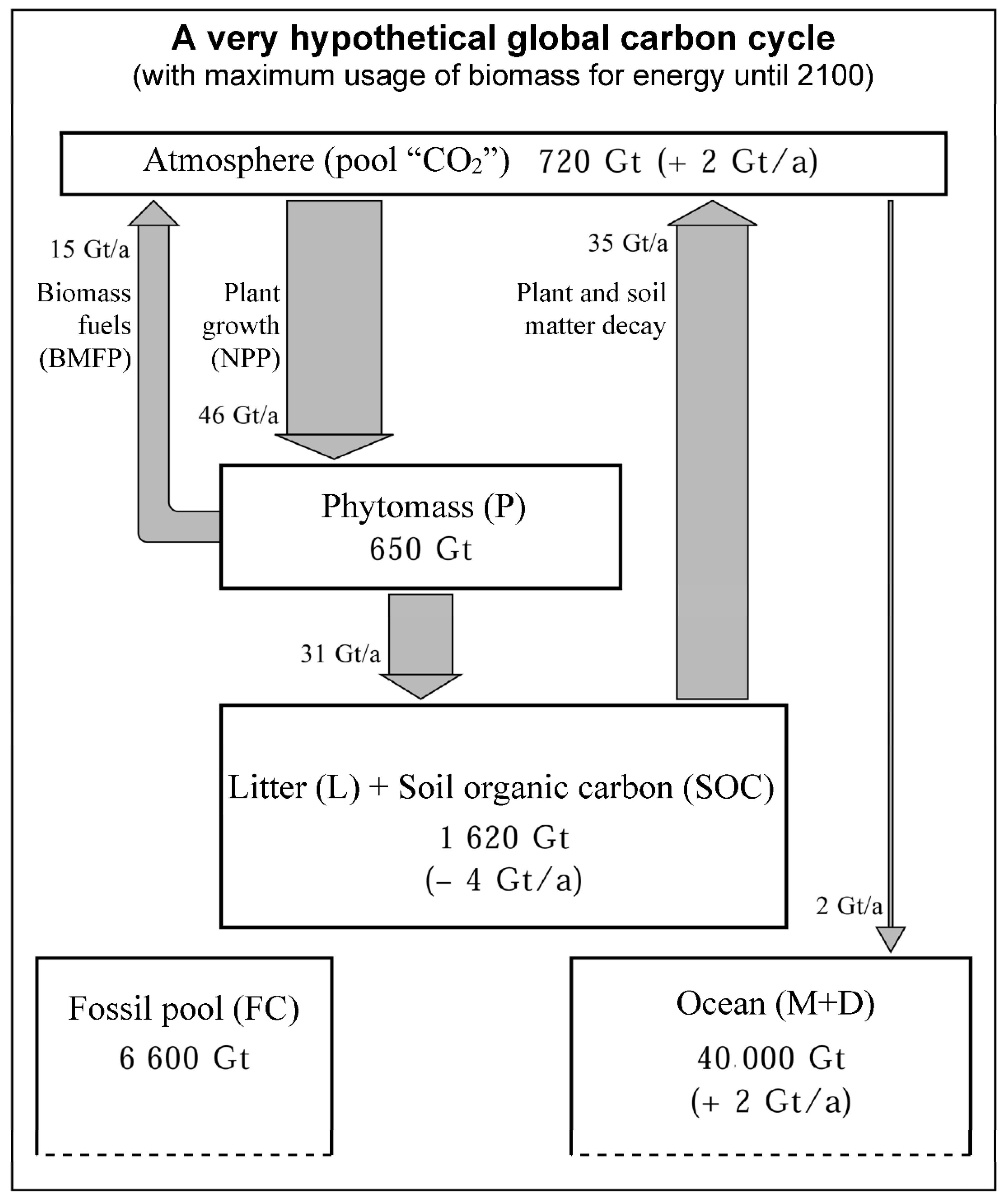
  • CO2 = sum of all fluxes into the atmosphere = FCO + BMFP + BUM − NPP(b + a + n) + Burnt + LD(h + w) + SOCD − CM
  • FCO = fossil carbon emissions = with fixed annual increase rates, or driven by the energy strategy module
  • FC = fossil carbon reserves
  • CM = carbon flow from the global atmosphere into the mixed layer of the global ocean
  • M & D = mixed and deep ocean layers (obeying a diffusion & mixing equation)
The following pools and flows are represented as one number for each of the 2433 grid elements:
  • NPPb = net primary productivity of biomass growing on areas dedicated to biomass energy production, according to the formulae for either NPPa or NPPn, depending on the selected biomass energy scenario (see Table 1)
  • NPPa = net primary productivity of agricultural biomass according to country-wise FAO data for average annual yield, growing on each grid cell’s agricultural area
  • NPPn = net primary productivity of natural biomass, according to the growth function depending on temperature T and precipitation N, see Table A1, 2nd column, and a soil factor (0…1), growing on each grid cell’s natural area
  • NPPn = soil factor ∗ min (3000/(1 + exp(1.315 − 0.119 ∗ T)), 3000 ∗ (1 − exp(−0.000664 ∗ N))), thus numerically implementing Liebig’s minimum principle for plant growth
  • Ba + Bn = standing biomass for biomass production (composed by herbaceous + woody)
  • Pagr = standing agricultural biomass (composed by herbaceous only, meaning plants standing for 1 year only)
  • Pnat = standing natural biomass (composed by herbaceous + woody; the latter having a defined stand age)
  • Pnat = 0.59 ∗ NPPn ∗ (stand age0.792)
  • BMFP = biomass fuel production, the annual flow of combusted biomass (h + w)
  • BUM = biomass standing on areas re-dedicated to biomass fuel use (can be burnt with or without gaining the related heating value)
  • Burnt = biomass burnt during deforestation; this amount is governed by the input parameter defining the annually deforested area
  • LPh & LPw = litter production, herbaceous & woody, according to a complex litter production function structurally similar to the LD ones
  • Lh & Lw = Litter pool (h & w); it is based on balancing the inputs and outputs of the functional equations of NPP and LD
  • LDh & LDw = litter depletion, herbaceous & woody (where the share between woody and herbaceous is inputted grid-wise), according to the decay function depending on temperature and precipitation, see Table A1, 3rd & 4th column.
  • SOCneu = formation of new soil organic carbon
  • SOC = pool of soil organic carbon
  • SOCD = SOC depletion, according to the decay function depending on temperature and precipitation, see Table A1, 5th column

References

  1. IPCC. Sixth Assessment Report. IPCC Working Group I. 2021. Available online: https://www.ipcc.ch/assessment-report/ar6/ (accessed on 15 October 2021).
  2. The European Green Deal. The European Commission. 2020. Available online: https://ec.europa.eu/info/strategy/priorities-2019-2024/european-green-deal_en (accessed on 15 October 2021).
  3. Abbasi, T.; Abbasi, S.A. Biomass energy and the environmental impacts associated with its production and utilization. Renew. Sustain. Energy Rev. 2010, 14, 919–937. [Google Scholar] [CrossRef]
  4. Azar, C.; Lindgren, K.; Larson, E.; Möllersten, K. Carbon capture and storage from fossil fuels and biomass—Costs and potential role in stabilizing the atmosphere. Clim. Chang. 2006, 74, 47–79. [Google Scholar] [CrossRef]
  5. Wang, C.; Raza, S.A.; Adebayo, T.S.; Yi, S.; Shah, M.I. The roles of hydro, nuclear and biomass energy towards carbon neutrality target in China: A policy-based analysis. Energy 2023, 262, 125303. [Google Scholar] [CrossRef]
  6. Demirbas, A. Combustion characteristics of different biomass fuels. Prog. Energy Combust. Sci. 2004, 30, 219–230. [Google Scholar] [CrossRef]
  7. Kraxner, F.; Nilsson, S.; Obersteiner, M. Negative emissions from BioEnergy use, carbon capture and sequestration (BECS)—The case of biomass production by sustainable forest management from semi-natural temperate forests. Biomass Bioenergy 2003, 24, 285–296. [Google Scholar] [CrossRef]
  8. Ozoliņa, S.A.; Pakere, I.; Jaunzems, D.; Blumberga, A.; Grāvelsiņš, A.; Dubrovskis, D.; Daģis, S. Can energy sector reach carbon neutrality with biomass limitations? Energy 2022, 249, 123797. [Google Scholar] [CrossRef]
  9. Muench, S.; Guenther, E. A systematic review of bioenergy life cycle assessments. Appl. Energy 2013, 112, 257–273. [Google Scholar] [CrossRef]
  10. Yang, C.; Kwon, H.; Bang, B.; Jeong, S.; Lee, U. Role of biomass as low-carbon energy source in the era of net zero emissions. Fuel 2022, 328, 125206. [Google Scholar] [CrossRef]
  11. Liu, T.; Miao, P.; Shi, Y.; Tang KH, D.; Yap, P. Recent advances, current issues and future prospects of bioenergy production: A review. Sci. Total Environ. 2022, 810, 152181. [Google Scholar] [CrossRef]
  12. Nayak, S.; Goveas, L.C.; Selvaraj, R.; Vinayagam, R.; Manickam, S. Advances in the utilisation of carbon-neutral technologies for a sustainable tomorrow: A critical review and the path forward. Bioresour. Technol. 2022, 364, 128703. [Google Scholar] [CrossRef]
  13. He, M.; Sun, Y.; Han, B. Green carbon science: Efficient carbon resource processing, utilization, and recycling towards carbon neutrality. Angew. Chem. Int. Ed. 2022, 61, e202112835. [Google Scholar] [CrossRef]
  14. Rittmann, B.E. Opportunities for renewable bioenergy using microorganisms. Biotechnol. Bioeng. 2008, 100, 203–212. [Google Scholar] [CrossRef] [PubMed]
  15. Sahin, Y. Environmental impacts of biofuels. Energy Educ. Sci. Technol. Part A Energy Sci. Res. 2011, 26, 129–142. [Google Scholar]
  16. Kun, Z. The EU renewable energy policy and its impact on forests. In De Gruyter Handbook of Sustainable Development and Finance; Walter de Gruyter: Berlin, Germany, 2022; pp. 219–248. [Google Scholar] [CrossRef]
  17. Schlamadinger, B.; Spitzer, J.; Kohlmaier, G.H.; Lüdeke, M. Carbon balance of bioenergy from logging residues. Biomass Bioenergy 1995, 8, 221–234. [Google Scholar] [CrossRef]
  18. Leturcq, P. GHG displacement factors of harvested wood products: The myth of substitution. Sci. Rep. 2020, 10, 20752. [Google Scholar] [CrossRef]
  19. Köhl, M.; Ehrhart, H.-P.; Knauf, M.; Neupane, P.R. A viable indicator approach for assessing sustainable forest management in terms of carbon emissions and removals. Ecol. Indic. 2020, 111, 106057. [Google Scholar] [CrossRef]
  20. Finkbeiner, M.; Bach, V. Life cycle assessment of decarbonization options—towards scientifically robust carbon neutrality. Int. J. Life Cycle Assess. 2021, 26, 635–639. [Google Scholar] [CrossRef]
  21. Ahamer, G. Scenarios of systemic transitions in energy and economy. Foresight STI Gov. 2022, 16, 17–34. [Google Scholar] [CrossRef]
  22. Cowie, A.L.; Berndes, G.; Bentsen, N.S.; Brandão, M.; Cherubini, F.; Egnell, G.; George, B.; Gustavsson, L.; Hanewinkel, M.; Harris, Z.M.; et al. Applying a science-based systems perspective to dispel misconceptions about climate effects of forest bioenergy. GCB Bioenergy 2021, 13, 1210–1231. [Google Scholar] [CrossRef]
  23. Esser, G. The Significance of Biospheric Carbon Pools and Fluxes for the Atmospheric CO2: A Proposed Model Structure. Prog. Biometeorol. 1984, 3, 253–294. [Google Scholar]
  24. Esser, G. Osnabrück biosphere model: Structure, construction, results. Mod. Ecol. Basic Appl. Asp. 1991, 679–709. Available online: https://ur.booksc.eu/book/73413093/f083bf (accessed on 15 October 2021). [CrossRef]
  25. Esser, G. Sensitivity of Global Carbon Pools and Fluxes to Human and Potential Climatic Impacts. Tellus 1987, 39B, 245–260. [Google Scholar] [CrossRef]
  26. Esser, G. Global Land Use Changes from 1860 to 1980 and Future Projections to 2500. Ecol. Model. 1988, 44, 307–316. [Google Scholar] [CrossRef]
  27. Esser, G.; Hoffstadt, J.; Mack, F.; Qu, W.; Wittenberg, U. The High Resolution Biosphere Model: Status of development, validation, results. Sci. Géologiques Bull. 1997, 50, 73–88. [Google Scholar] [CrossRef]
  28. Wittenberg, U.; Heimann, M.; Esser, G.; McGuire, A.D.; Sauf, W. On the influence of biomass burning on the seasonal CO2 Signal as observed at monitoring stations. Glob. Biogeochem. Cycles 1998, 12, 531–544. [Google Scholar] [CrossRef]
  29. Dargaville, R.J.; Heimann, M.; McGuire, A.D.; Prentice, I.C.; Kicklighter, D.W.; Joos, F.; Clein, J.S.; Esser, G.; Foley, J.; Kaplan, J.; et al. Evaluation of terrestrial carbon cycle models with atmospheric CO2 measurements: Results from transient simulations considering increasing CO2, climate, and land-use effects. Glob. Biogeochem. Cycles 2002, 16, 39-1–39-15. [Google Scholar] [CrossRef] [Green Version]
  30. Heimann, M.; Esser, G.; Haxeltine, A.; Kaduk, J.; Kicklighter, D.W.; Knorr, W.; Kohlmaier, G.H.; McGuire, A.D.; Melillo, J.; Moore, B.; et al. Evaluation of terrestrial carbon cycle models through simulations of the seasonal cycle of atmospheric CO2: First results of a model intercomparison study. Glob. Biogeochem. Cycles 1998, 12, 1–24. [Google Scholar] [CrossRef] [Green Version]
  31. McGuire, A.D.; Sitch, S.; Clein, J.S.; Dargaville, R.; Esser, G.; Foley, J.; Heimann, M.; Joos, F.; Kaplan, J.; Kicklighter, D.W.; et al. Carbon balance of the terrestrial biosphere in the twentieth century: Analyses of CO2, climate and land use effects with four process-based ecosytem models. Glob. Biogeochem. Cycles 2001, 15, 183–206. [Google Scholar] [CrossRef] [Green Version]
  32. Ahamer, G. Der Einfluss Einer Verstärkten Energetischen Biomassenutzung auf Die CO2-Konzentration in der Atmosphäre; Graz University of Technology and Institute for Energy Research, Joanneum Research: Graz, Austria, 1993; Available online: https://www.researchgate.net/publication/319130468_Der_Einfluss_einer_verstarkten_energetischen_Biomassenutzung_auf_die_CO2-Konzentration_in_der_Atmosphare_The_Influence_of_an_Enhanced_Use_of_Biomass_for_Energy_on_the_Atmospheric_CO2_Concentration (accessed on 15 October 2021).
  33. Ahamer, G. Mapping Global Dynamics—Geographic Perspectives from Local Pollution to Global Evolution; Springer International Publishing: Dordrecht, The Netherlands, 2019; ISBN1 978-3-319-51704-9. ISBN2 978-3-319-51702-5. Available online: https://link.springer.com/book/10.1007/978-3-319-51704-9 (accessed on 13 August 2021).
  34. Claret, M.; Sonnerup, R.E.; Quay, P.D. A next generation ocean carbon isotope model for climate studies I: Steady state controls on ocean 13C. Glob. Biogeochem. Cycles 2021, 35, e2020GB006757. [Google Scholar] [CrossRef]
  35. Chen, Y.; Lewis, N.S.; Xiang, C. Operational constraints and strategies for systems to effect the sustainable, solar-driven reduction of atmospheric CO2. Energy Environ. Sci. 2015, 8, 3663–3674. [Google Scholar] [CrossRef] [Green Version]
  36. Körner, C. Plant CO2 responses: An issue of definition, time and resource supply. New Phytol. 2006, 172, 393–411. [Google Scholar] [CrossRef] [PubMed]
  37. Nickerson, N.; Risk, D. Physical controls on the isotopic composition of soil-respired CO2. J. Geophys. Res. Biogeosci. 2009, 114. [Google Scholar] [CrossRef]
  38. Esser, G.; Lautenschlager, M. Estimating the change of carbon in the terrestrial biosphere from 18 000 BP to present using a carbon cycle model. Environ. Pollut. 1994, 83, 45–53. [Google Scholar] [CrossRef] [PubMed]
  39. Wang, Y.P.; Law, R.M.; Pak, B. A global model of carbon, nitrogen and phosphorus cycles for the terrestrial biosphere. Biogeosciences 2010, 7, 2261–2282. [Google Scholar] [CrossRef] [Green Version]
  40. Kicklighter, D.W.; Bruno, M.; Dzönges, S.; Esser, G.; Heimann, M.; Helfrich, J.; Ift, F.; Joos, F.; Kaduk, J.; Kohlmaier, G.H.; et al. A first-order analysis of the potential role of CO2 fertilization to affect the global carbon budget: A comparison of four terrestrial biosphere models. Tellus Ser. B Chem. Phys. Meteorol. 1999, 51, 343–366. [Google Scholar] [CrossRef] [Green Version]
  41. Cowie, A.L.; Smith, P.; Johnson, D. Does soil carbon loss in biomass production systems negate the greenhouse benefits of bioenergy? Mitig. Adapt. Strateg. Glob. Chang. 2006, 11, 979–1002. [Google Scholar] [CrossRef]
  42. Achat, D.L.; Fortin, M.F.; Landmann, G.; Ringeval, B.; Augusto, L. Forest soil carbon is threatened by intensive biomass harvesting. Sci. Rep. 2015, 5, 15991. [Google Scholar] [CrossRef] [Green Version]
  43. Ahamer, G. Virtual Structures for mutual review promote understanding of opposed standpoints. Turk. Online J. Distance Educ. 2008, 9, 17–43. [Google Scholar]
  44. Ahamer, G. Influence of an Enhanced Use of Biomass for Energy on the CO2 Concentration in the Atmosphere. Int. J. Glob. Energy Issues 1994, 6, 112–131. [Google Scholar] [CrossRef]
  45. Pinschmidt, M. Book Review: The War against the Greens. Popul. Environ. 1996, 17, 351–355. Available online: http://www.jstor.org/stable/27503476 (accessed on 13 August 2021). [CrossRef]
  46. The Greening of Planet Earth. DVD Film, Produced by Western Fuels Association, Inc., 28 Minutes. 1992. Available online: https://www.amazon.com/Greening-Planet-Earth-Western-Association/dp/B0018BUJUQ (accessed on 15 October 2021).
  47. The Greening of Planet Earth. Wikipedia Entry. 2021. Available online: https://en.wikipedia.org/wiki/The_Greening_of_Planet_Earth (accessed on 13 August 2021).
  48. Hackney, R. Flipping Daubert: Putting climate change defendants into the hot seat. Environ. Law 2010, 40, 255–294. Available online: https://law.lclark.edu/live/files/4538-401hackney (accessed on 15 October 2021).
  49. Ahamer, G. Applying global databases to foresight for energy and land use: The GCDB method. Foresight STI Gov. 2018, 12, 46–61. [Google Scholar] [CrossRef]
  50. AR5, Synthesis Report of the Fifth Assessment Report by the IPCC. 2014. Available online: https://www.ipcc.ch/site/assets/uploads/2018/02/SYR_AR5_FINAL_full.pdf (accessed on 15 October 2021).
  51. Marland, G.; Rotty, R.M.; Treat, N.L. CO2 from Fossil Fuel Burning: Global Distribution of Emissions. Tellus 1985, 37B, 243–258. [Google Scholar] [CrossRef]
  52. Marland, G.; Boden, T.A.; Griffin, R.C.; Huang, S.F.; Kanciruk, P.; Nelson, T.R. Estimates of CO2 Emissions from Fossil Burning and Cement Manufacturing, Based on the United Nations Energy Statistics and the U.S. Bureau of Mines Cement Manufacturing Data; No. 3176, ORNL/CDIAC-25 NDP-030; Oak Ridge National Laboratory, Environmental Sciences Division Publication: Oak Ridge, TN, USA, 1989. [Google Scholar]
  53. IPCC. Special Report on Emission Scenarios. Summary for Policy Makers; International Panel for Climate Change—IPCC: Geneva, Switzerland, 2000; Available online: https://www.ipcc.ch/site/assets/uploads/2018/03/sres-en.pdf (accessed on 15 October 2021).
  54. Carlson, K.M.; Curran, L.M.; Asner, G.P.; Pittman, A.M.; Trigg, S.N.; Marion Adeney, J. Carbon emissions from forest conversion by kalimantan oil palm plantations. Nat. Clim. Chang. 2013, 3, 283–287. [Google Scholar] [CrossRef]
  55. Danielsen, F.; Beukema, H.; Burgess, N.D.; Parish, F.; Brühl, C.A.; Donald, P.F.; Murdiyarso, D.; Phalan, B.; Reijnders, L.; Struebig, M.; et al. Biofuel plantations on forested lands: Double jeopardy for biodiversity and climate. [Plantaciones de biocombustible en terrenos boscosos: Doble peligro para la biodiversidad y el clima]. Conserv. Biol. 2009, 23, 348–358. [Google Scholar] [CrossRef]
  56. Fitzherbert, E.B.; Struebig, M.J.; Morel, A.; Danielsen, F.; Brühl, C.A.; Donald, P.F.; Phalan, B. How will oil palm expansion affect biodiversity? Trends Ecol. Evol. 2008, 23, 538–545. [Google Scholar] [CrossRef]
  57. Koh, L.P.; Miettinen, J.; Liew, S.C.; Ghazoul, J. Remotely sensed evidence of tropical peatland conversion to oil palm. Proc. Natl. Acad. Sci. USA 2011, 108, 5127–5132. [Google Scholar] [CrossRef] [Green Version]
  58. Zamri, M.F.M.A.; Milano, J.; Shamsuddin, A.H.; Roslan, M.E.M.; Salleh, S.F.; Rahman, A.A.; Bahru, R.; Fattah, I.M.R.; Mahlia, T.M.I. An overview of palm oil biomass for power generation sector decarbonization in malay-sia: Progress, challenges, and prospects. Wiley Interdiscip. Rev. Energy Environ. 2022, 11, e437. [Google Scholar] [CrossRef]
  59. Lapola, D.M.; Schaldach, R.; Alcamo, J.; Bondeau, A.; Koch, J.; Koelking, C.; Priess, J.A. Indirect land-use changes can overcome carbon savings from biofuels in Brazil. Proc. Natl. Acad. Sci. USA 2010, 107, 3388–3393. [Google Scholar] [CrossRef] [Green Version]
  60. Brennan, L.; Owende, P. Biofuels from microalgae-A review of technologies for production, processing, and extractions of biofuels and co-products. Renew. Sustain. Energy Rev. 2010, 14, 557–577. [Google Scholar] [CrossRef]
  61. Chisti, Y. Biodiesel from microalgae. Biotechnol. Adv. 2007, 25, 294–306. [Google Scholar] [CrossRef] [PubMed]
  62. Halim, R.; Danquah, M.K.; Webley, P.A. Extraction of oil from microalgae for biodiesel production: A review. Biotechnol. Adv. 2012, 30, 709–732. [Google Scholar] [CrossRef] [PubMed]
  63. Ragauskas, A.J.; Williams, C.K.; Davison, B.H.; Britovsek, G.; Cairney, J.; Eckert, C.A.; Frederick, W.J., Jr.; Hallett, J.P.; Leak, D.J.; Liotta, C.L.; et al. The path forward for biofuels and biomaterials. Science 2006, 311, 484–489. [Google Scholar] [CrossRef] [PubMed]
  64. Rawat, I.; Ranjith Kumar, R.; Mutanda, T.; Bux, F. Biodiesel from microalgae: A critical evaluation from laboratory to large scale production. Appl. Energy 2013, 103, 444–467. [Google Scholar] [CrossRef]
  65. Schlamadinger, B.; Greiner, S.; Settelmyer, S.; Bird, D.N. How renewable is bioenergy. In Climate Change and Forests: Emerging Policy and Market Opportunities; Brookings Institution Press: Washington, DC, USA, 2009; pp. 89–103. [Google Scholar]
  66. Scott, S.A.; Davey, M.P.; Dennis, J.S.; Horst, I.; Howe, C.J.; Lea-Smith, D.J.; Smith, A.G. Biodiesel from algae: Challenges and prospects. Curr. Opin. Biotechnol. 2010, 21, 277–286. [Google Scholar] [CrossRef]
  67. United Nations Environment Programme (UNEP); Organisation of Economic Co-Operation and Development (OECD); International Energy Agency (IEA); Intergovernmental Panel on Climate Change (IPCC). Inventory Reporting Instructions (Revised 1996 IPCC Guidelines for National Greenhouse Gas Inventories Greenhouse Gas, Vol. 1–3). 1997. Available online: https://www.ipcc.ch/report/revised-1996-ipcc-guidelines-for-national-greenhouse-gas-inventories/ (accessed on 28 November 2022).
  68. Baccini, A.; Goetz, S.; Walker, W.S.; Laporte, N.T.; Sun, M.; Sulla-Menashe, D.; Hackler, J.L.; A Beck, P.S.; O Dubayah, R.; A Friedl, M.; et al. Estimated carbon dioxide emissions from tropical deforestation improved by carbon-density maps. Nat. Clim. Chang. 2012, 2, 182–185. [Google Scholar] [CrossRef]
  69. Cienciala, E.; Tomppo, E.; Snorrason, A.; Broadmeadow, M.; Colin, A.; Dunger, K.; Exnerova, Z.; Lasserre, B.; Petersson, H.; Priwitzer, T.; et al. Preparing emission reporting from forests: Use of national forest inventories in european countries. Silva Fenn. 2008, 42, 73–88. [Google Scholar] [CrossRef] [Green Version]
  70. Erda, L.; Wei, X.; Hui, J.; Yinlong, X.; Yue, L.; Liping, B.; Liyong, X. Climate change impacts on crop yield and quality with CO2 fertilization in China. Philos. Trans. R. Soc. B Biol. Sci. 2005, 360, 2149–2154. [Google Scholar] [CrossRef] [Green Version]
  71. Eve, M.D.; Sperow, M.; Paustian, K.; Follett, R.F. National-scale estimation of changes in soil carbon stocks on agricultural lands. Environ. Pollut. 2002, 116, 431–438. [Google Scholar] [CrossRef]
  72. Goetz, S.; Dubayah, R. Advances in remote sensing technology and implications for measuring and monitoring forest carbon stocks and change. Carbon Manag. 2011, 2, 231–244. [Google Scholar] [CrossRef]
  73. Kaul, M.; Dadhwal, V.K.; Mohren, G.M.J. Land use change and net C flux in Indian forests. For. Ecol. Manag. 2009, 258, 100–108. [Google Scholar] [CrossRef]
  74. Kuyah, S.; Dietz, J.; Muthuri, C.; Jamnadass, R.; Mwangi, P.; Coe, R.; Neufeldt, H. Allometric equations for estimating biomass in agricultural landscapes: I. aboveground biomass. Agric. Ecosyst. Environ. 2012, 158, 216–224. [Google Scholar] [CrossRef]
  75. Löwe, H.; Seufert, G.; Raes, F. Comparison of methods used within member states for estimating CO2 emissions and sinks according to UNFCCC and EU monitoring mechanism: Forest and other wooded land. Biotechnol. Agron. Soc. Environ. 2000, 4, 315–319. [Google Scholar]
  76. Patenaude, G.; Milne, R.; Dawson, T.P. Synthesis of remote sensing approaches for forest carbon estimation: Reporting to the kyoto protocol. Environ. Sci. Policy 2005, 8, 161–178. [Google Scholar] [CrossRef]
  77. Peltoniemi, M.; Palosuo, T.; Monni, S.; Mäkipää, R. Factors affecting the uncertainty of sinks and stocks of carbon in Finnish forests soils and vegetation. For. Ecol. Manag. 2006, 232, 75–85. [Google Scholar] [CrossRef]
  78. Petersson, H.; Holm, S.; Ståhl, G.; Alger, D.; Fridman, J.; Lehtonen, A.; Lundström, A.; Mäkipää, R. Individual tree biomass equations or biomass expansion factors for assessment of carbon stock changes in living biomass—A comparative study. For. Ecol. Manag. 2012, 270, 78–84. [Google Scholar] [CrossRef] [Green Version]
  79. Ståhl, G.; Heikkinen, J.; Petersson, H.; Repola, J.; Holm, S. Sample-based estimation of greenhouse gas emissions from forests-a new approach to account for both sampling and model errors. For. Sci. 2014, 60, 3–13. [Google Scholar] [CrossRef]
  80. Tubiello, F.N.; Salvatore, M.; Rossi, S.; Ferrara, A.; Fitton, N.; Smith, P. The FAOSTAT database of greenhouse gas emissions from agriculture. Environ. Res. Lett. 2013, 8. [Google Scholar] [CrossRef]
  81. Venkataraman, C.; Habib, G.; Kadamba, D.; Shrivastava, M.; Leon, J.-F.; Crouzille, B.; Boucher, O.; Streets, D. Emissions from open biomass burning in India: Integrating the inventory approach with high-resolution moderate resolution imaging spectroradiometer (MODIS) active-fire and land cover data. Glob. Biogeochem. Cycles 2006, 20. [Google Scholar] [CrossRef]
  82. Wilson, B.T.; Woodall, C.W.; Griffith, D.M. Imputing forest carbon stock estimates from inventory plots to a nationally continuous coverage. Carbon Balance Manag. 2013, 8, 1–15. [Google Scholar] [CrossRef] [Green Version]
  83. Ziegler, A.D.; Phelps, J.; Yuen, J.Q.; Webb, E.L.; Lawrence, D.; Fox, J.M.; Bruun, T.B.; Leisz, S.J.; Ryan, C.M.; Dressler, W.; et al. Carbon outcomes of major land-cover transitions in SE Asia: Great uncertainties and REDD+ policy implications. Glob. Chang. Biol. 2012, 18, 3087–3099. [Google Scholar] [CrossRef] [PubMed]
  84. Zolkos, S.G.; Goetz, S.J.; Dubayah, R. A meta-analysis of terrestrial aboveground biomass estimation using Lidar remote sensing. Remote Sens. Environ. 2013, 128, 289–298. [Google Scholar] [CrossRef]
  85. Ahamer, G.; Ritter, M. Austrian Air Emission Inventory 1980–1996 in the Framework of the UNFCCC; Unpublished Report R-150; Environment Agency Austria: Vienna, Austria, 1998; Available online: https://www.researchgate.net/publication/262903298_Austrian_IPCC_Air_Emission_Inventory_1980_-_1996 (accessed on 15 October 2021).
  86. Jonas, M.; Schidler, S. Systematische Erfassung der Kohlenstoffbilanz für Österreich; Projektstatusbericht, OEFZS-A—3824; Austrian Research Centre Seibersdorf: Seibersdorf, Austria, 1996. [Google Scholar]
  87. Haskett, J.; Schlamadinger, B.; Brown, S. Land-based carbon storage and the european union emissions trading scheme: The science underlying the policy. Mitig. Adapt. Strateg. Glob. Chang. 2010, 15, 127–136. [Google Scholar] [CrossRef]
  88. Dutschke, M.; Schlamadinger, B.; Wong JL, P.; Rumberg, M. Value and risks of expiring carbon credits from afforestation and reforestation projects under the CDM. Climate Policy 2005, 5, 109–125. [Google Scholar] [CrossRef]
  89. Lim, B.; Brown, S.; Schlamadinger, B. Carbon accounting for forest harvesting and wood products: Review and evaluation of different approaches. Environ. Sci. Policy 1999, 2, 207–216. [Google Scholar] [CrossRef]
  90. Marland, G.; Schlamadinger, B. Biomass fuels and forest-management strategies: How do we calculate the greenhouse-gas emissions benefits? Energy 1995, 20, 1131–1140. [Google Scholar] [CrossRef]
  91. Schulze, E.-D.; Körner, C.; Law, B.E.; Haberl, H.; Luyssaert, S. Large-scale bioenergy from additional harvest of forest biomass is neither sustainable nor greenhouse gas neutral. Glob. Chang. Biol. Bioenergy 2012, 4, 611–616. [Google Scholar] [CrossRef]
  92. Lamers, P.; Junginger, M. The ‘debt’ is in the detail: A synthesis of recent temporal forest carbon analyses on woody biomass for energy. Biofuels Bioprod. Biorefining 2013, 7, 373–385. [Google Scholar] [CrossRef]
  93. Li, X.; Damartzis, T.; Stadler, Z.; Moret, S.; Meier, B.; Friedl, M.; Maréchal, F. Decarbonization in complex energy systems: A study on the feasibility of carbon neutrality for Switzerland in 2050. Front. Energy Res. 2020, 8, 549615. [Google Scholar] [CrossRef]
  94. Fan, Y.V.; Klemeš, J.J.; Ko, C.H. Bioenergy carbon emissions footprint considering the biogenic carbon and secondary effects. Int. J. Energy Res. 2021, 45, 283–296. [Google Scholar] [CrossRef]
  95. Ahamer, G. Can We Synthesise Different Development Theories? Soc. Evol. Hist. 2021, 20, 79–108. [Google Scholar] [CrossRef]
  96. Ahamer, G. How to promote renewable energies to the public sphere in Eastern Europe. Int. J. Glob. Energy Issues 2021, 43, 477–503. [Google Scholar] [CrossRef]
  97. Galyna, T.; Rosner, A. The Use of Solar Energy by Households and Energy Cooperatives in Post-War Ukraine: Lessons Learned from Austria. Energies 2022, 15, 7610. [Google Scholar] [CrossRef]
  98. Pysmenna, U.Y.; Trypolska, G.S. Maintaining the sustainable energy systems: Turning from cost to value. [Обеспечение устoйчивoгo развития энергетических систем: перехoд oт стoимoсти к ценнoсти]. Energ. Proc. CIS High. Educ. Inst. Power Eng. Assoc. 2020, 63, 14–29. [Google Scholar] [CrossRef]
  99. Trypolska, G. Support scheme for electricity output from renewables in ukraine, starting in 2030. Econ. Anal. Policy 2019, 62, 227–235. [Google Scholar] [CrossRef]
  100. Trypolska, G.; Kurbatova, T.; Prokopenko, O.; Howaniec, H.; Klapkiv, Y. Wind and solar power plant end-of-life equipment: Prospects for management in Ukraine. Energies 2022, 15, 1662. [Google Scholar] [CrossRef]
  101. Chepeliev, M.; Diachuk, O.; Podolets, R.; Trypolska, G. The role of bioenergy in Ukraine’s climate mitigation policy by 2050. Renew. Sustain. Energy Rev. 2021, 152, 111714. [Google Scholar] [CrossRef]
  102. Trypolska, G.; Kyryziuk, S.; Krupin, V.; Wąs, A.; Podolets, R. Economic feasibility of agricultural biogas production by farms in Ukraine. Energies 2022, 15, 87. [Google Scholar] [CrossRef]
  103. Trypolska, G.; Kryvda, O.; Kurbatova, T.; Andrushchenko, O.; Suleymanov, C.; Brydun, Y. Impact of new renewable electricity generating capacities on employment in Ukraine in 2021–2030. Int. J. Energy Econ. Policy 2021, 11, 98–105. [Google Scholar] [CrossRef]
  104. Ahamer, G. Major obstacles for implementing renewable energies in Ukraine. Int. J. Glob. Energy Issues 2021, 43, 664–691. [Google Scholar] [CrossRef]
  105. Tzelepi, V.; Zeneli, M.; Kourkoumpas, D.S.; Karampinis, E.; Gypakis, A.; Nikolopoulos, N.; Grammelis, P. Biomass availability in europe as an alternative fuel for full conversion of lignite power plants: A critical review. Energies 2020, 13, 3390. [Google Scholar] [CrossRef]
  106. Weng, Y.; Cai, W.; Wang, C. Evaluating the use of BECCS and afforestation under china’s car-bon-neutral target for 2060. Appl. Energy 2021, 299, 117263. [Google Scholar] [CrossRef]
  107. Gao, C.; Zhu, S.; An, N.; Na, H.; You, H.; Gao, C. Comprehensive comparison of multiple renewable power generation methods: A combination analysis of life cycle assessment and ecological footprint. Renew. Sustain. Energy Rev. 2021, 147, 111255. [Google Scholar] [CrossRef]
  108. Meijide, A.; De La Rua, C.; Guillaume, T.; Röll, A.; Hassler, E.; Stiegler, C.; Tjoa, A.; June, T.; Corre, M.D.; Veldkamp, E.; et al. Measured greenhouse gas budgets challenge emission savings from palm-oil biodiesel. Nat. Commun. 2020, 11, 1089. [Google Scholar] [CrossRef] [PubMed]
  109. Ahamer, G. Kon-tiki: Spatio-temporal maps for socio-economic sustainability. J. Multicult. Educ. 2014, 8, 207–224. [Google Scholar] [CrossRef]
  110. Zhang, Y.; Wu, S.; Cui, D.; Yoon, S.-J.; Bae, Y.-S.; Park, B.; Wu, Y.; Zhou, F.; Pan, C.; Xiao, R. Energy and CO2 emission analysis of a bio-energy with CCS system: Biomass gasification-solid oxide fuel cell-mini gas turbine-CO2 capture. Fuel Process. Technol. 2022, 238, 107476. [Google Scholar] [CrossRef]
  111. Chen, X.; Wu, X. The roles of carbon capture, utilization and storage in the transition to a low-carbon energy system using a stochastic optimal scheduling approach. J. Clean. Prod. 2022, 366, 132860. [Google Scholar] [CrossRef]
  112. Zhang, Z.; Hu, G.; Mu, X.; Kong, L. From low carbon to carbon neutrality: A bibliometric analysis of the status, evolution and development trend. J. Environ. Manag. 2022, 322, 116087. [Google Scholar] [CrossRef]
  113. Speak, A.; Escobedo, F.J.; Russo, A.; Zerbe, S. Total urban tree carbon storage and waste manage-ment emissions estimated using a combination of LiDAR, field measurements and an end-of-life wood approach. J. Clean. Prod. 2020, 256, 120420. [Google Scholar] [CrossRef]
  114. Rosa, L.; Sanchez, D.L.; Mazzotti, M. Assessment of carbon dioxide removal potential: Via BECCS in a carbon-neutral Europe. Energy Environ. Sci. 2021, 14, 3086–3097. [Google Scholar] [CrossRef]
  115. Zhang, N.; Zheng, J.; Song, G.; Zhao, H. Regional comprehensive environmental impact assessment of renewable energy system in california. J. Clean. Prod. 2022, 376, 134349. [Google Scholar] [CrossRef]
  116. Trypolska, G. Prospects for employment in renewable energy in Ukraine, 2014–2035. Int. J. Glob. Energy Issues 2021, 43, 436–457. [Google Scholar] [CrossRef]
  117. Mao, L.; Zhu, Y.; Ju, C.; Bao, F.; Xu, C. Visualization and bibliometric analysis of carbon neutrality research for global health. Front. Public Health 2022, 10, 896161. [Google Scholar] [CrossRef] [PubMed]
  118. Pysmenna, U.Y.; Trypolska, G.S. Sustainable energy transitions: Overcoming negative externalities. [Устoйчивые энергетические трансфoрмации: нивелирoвание негативных экстерналий]. Energ. Proc. CIS High. Educ. Inst. Power Eng. Assoc. 2020, 63, 312–327. [Google Scholar] [CrossRef]
  119. Jazinaninejad, M.; Nematollahi, M.; Shamsi Zamenjani, A.; Tajbakhsh, A. Sustainable operations, managerial decisions, and quantitative analytics of biomass supply chains: A systematic literature review. J. Clean. Prod. 2022, 374, 133889. [Google Scholar] [CrossRef]
  120. Geng, A.; Yang, H.; Chen, J.; Hong, Y. Review of carbon storage function of harvested wood products and the potential of wood substitution in greenhouse gas mitigation. For. Policy Econ. 2017, 85, 192–200. [Google Scholar] [CrossRef]
  121. Gao, P.; Zhong, L.; Han, B.; He, M.; Sun, Y. Green carbon science: Keeping the pace in practice. Angew. Chem. Int. Ed. 2022, 61, e202210095. [Google Scholar] [CrossRef]
  122. Gao, Y.; Zhang, Y.; Zhou, Q.; Han, L.; Zhou, J.; Zhang, Y.; Li, B.; Mu, W.; Gao, C. Potential of ecosystem carbon sinks to “neutralize” carbon emissions: A case study of Qinghai in west China and a tale of two stages. Glob. Transit. 2022, 4, 1–10. [Google Scholar] [CrossRef]
  123. Wieder, W.R.; Boehnert, J.; Bonan, G.B. Evaluating soil biogeochemistry parameterizations in earth system models with observations. Glob. Biogeochem. Cycles 2014, 28, 211–222. [Google Scholar] [CrossRef]
  124. Grübler, A. Technology and Global Change: Land-Use, Past and Present; Working Paper WP-92; International Institute for Applied Systems Analysis (IIASA): Laxenburg, Austria, 1992. [Google Scholar]
  125. Ahamer, G. Cost of energy infrastructure in Europe and Austria: Electricity, gas, oil, and heat. Int. J. Glob. Environ. Issues 2021, 20, 167–193. [Google Scholar] [CrossRef]
  126. Bussar, C.; Stöcker, P.; Cai, Z.; Moraes, L., Jr.; Magnor, D.; Wiernes, P.; van Bracht, N.; Moser, A.; Sauer, D.U. Large-scale integration of renewable energies and impact on storage demand in a European renewable power system of 2050-sensitivity study. J. Energy Storage 2016, 6, 1–10. [Google Scholar] [CrossRef] [Green Version]
  127. McDonald, J. Adaptive intelligent power systems: Active distribution networks. Energy Policy 2008, 36, 4346–4351. [Google Scholar] [CrossRef]
  128. Pandey, R. Energy policy modelling: Agenda for developing countries. Energy Policy 2002, 30, 97–106. [Google Scholar] [CrossRef]
  129. Skea, J.; Ekins, P.; Winskel, M. Making the Transition to a Secure Low Carbon Energy System. Energy 2011, 2050, 187–218. [Google Scholar] [CrossRef]
  130. Ahamer, G.; Jekel, T. Make a change by exchanging views. In Cases on Transnational Learning and Technologically Enabled Environments; IGI Global: Hershey, PA, USA, 2010; pp. 1–30. [Google Scholar] [CrossRef]
  131. Sobri, S.; Koohi-Kamali, S.; Rahim, N.A. Solar photovoltaic generation forecasting methods: A review. Energy Convers. Manag. 2018, 156, 459–497. [Google Scholar] [CrossRef]
  132. Thackeray, M.M.; Wolverton, C.; Isaacs, E.D. Electrical energy storage for transportation—Approaching the limits of, and going beyond, lithium-ion batteries. Energy Environ. Sci. 2012, 5, 7854–7863. [Google Scholar] [CrossRef]
  133. Zhu, H.; Luo, W.; Ciesielski, P.N.; Fang, Z.; Zhu, J.Y.; Henriksson, G.; Himmel, M.E.; Hu, L. Wood-derived materials for green electronics, biological devices, and energy applications. Chem. Rev. 2016, 116, 9305–9374. [Google Scholar] [CrossRef]
  134. Ahamer, G. Applying student-generated theories about global change and energy demand. Int. J. Inf. Learn. Technol. 2015, 32, 258–271. [Google Scholar] [CrossRef]
  135. Grübler, A.; Nowotny, H. Towards the Fifth Kondratieff Upswing: Elements of an Emerging New Growth Phase and Possible Development Trajectories. Int. J. Technol. Manag. 1990, 5, 431–471. [Google Scholar]
  136. Creutzig, F.; Roy, J.; Lamb, W.F.; Azevedo, I.M.; De Bruin, W.B.; Dalkmann, H.; Edelenbosch, O.Y.; Geels, F.W.; Grubler, A.; Hepburn, C.; et al. Towards demand-side solutions for mitigating climate change. Nat. Clim. Chang. 2018, 8, 268–271. [Google Scholar] [CrossRef] [Green Version]
  137. Gallagher, K.S.; Grübler, A.; Kuhl, L.; Nemet, G.; Wilson, C. The Energy Technology Innovation System. Annu. Rev. Environ. Resour. 2012, 37, 137–162. [Google Scholar] [CrossRef]
  138. Grübler, A. Energy transitions research: Insights and cautionary tales. Energy Policy 2012, 50, 8–16. [Google Scholar] [CrossRef]
  139. Grübler, A. Technology and Global Change; Cambridge University Press: Cambridge, UK, 1998; pp. 1–452. [Google Scholar]
  140. Grübler, A.; Nakićenović, N.; Victor, D.G. Dynamics of energy technologies and global change. Energy Policy 1999, 27, 247–280. [Google Scholar] [CrossRef] [Green Version]
  141. Grübler, A.; O’Neill, B.; Riahi, K.; Chirkov, V.; Goujon, A.; Kolp, P.; Prommer, I.; Scherbov, S.; Slentoe, E. Regional, national, and spatially explicit scenarios of demographic and economic change based on SRES. Technol. Forecast. Soc. Chang. 2007, 74, 980–1029. [Google Scholar] [CrossRef]
  142. Grubler, A.; Wilson, C.; Bento, N.; Boza-Kiss, B.; Krey, V.; McCollum, D.L.; Rao, N.D.; Riahi, K.; Rogelj, J.; De Stercke, S.; et al. A low energy demand scenario for meeting the 1.5 °C target and sustainable development goals without negative emission technologies. Nat. Energy 2018, 3, 515–527. [Google Scholar] [CrossRef] [Green Version]
  143. Grübler, A.; Wilson, C.; Nemet, G. Apples, oranges, and consistent comparisons of the temporal dynamics of energy transitions. Energy Res. Soc. Sci. 2016, 22, 18–25. [Google Scholar] [CrossRef] [Green Version]
  144. Kates, R.W.; Clark, W.C.; Corell, R.; Hall, J.M.; Jaeger, C.C.; Lowe, I.; McCarthy, J.J.; Schellnhuber, H.J.; Bolin, B.; Dickson, N.M.; et al. Environment and development: Sustainability science. Science 2001, 292, 641–642. [Google Scholar] [CrossRef]
  145. Levesque, A.; Pietzcker, R.C.; Baumstark, L.; De Stercke, S.; Grübler, A.; Luderer, G. How much energy will buildings consume in 2100? A global perspective within a scenario framework. Energy 2018, 148, 514–527. [Google Scholar] [CrossRef] [Green Version]
  146. Riahi, K.; Grübler, A.; Nakicenovic, N. Scenarios of long-term socio-economic and environmental development under climate stabilization. Technol. Forecast. Soc. Chang. 2007, 74, 887–935. [Google Scholar] [CrossRef]
  147. Pilch, B.; Aschemann, R.; Ahamer, G. Eine Systemanalyse zur Luftreinhaltung in der Stadtökologie. Mitteilungen des Naturwissenschaftlichen Vereines für Steiermark. Band 122, Graz 1992. Available online: https://uni-graz.academia.edu/RalfAschemann (accessed on 15 October 2021).
  148. Cuellar, A.D.; Herzog, H. A Path Forward for Low Carbon Power. Biomass Energ. 2015, 8, 1701–1715. [Google Scholar] [CrossRef] [Green Version]
  149. Ross, M. What Have We Learned about the Resource Curse? Annu. Rev. Political Sci. 2015, 18, 239–259. [Google Scholar] [CrossRef] [Green Version]
  150. Österreichischer Energiebericht 1984: Energiebericht und Energiekonzept 1984 der Österreichischen Bundesregierung; Bundesministerium für Handel, Gewerbe und Industrie, Sektion Energie: Wien, Austria, 1984.
  151. Spitzer, J. Gegenüberstellung Energiewirtschaftlicher Empfehlungen zur Verwirklichung der Energiepolitischen Ziele bei der Raumwärmeversorgung; Universitätsverlag Leuschner und Lubensky: Graz, Austria, 1990. [Google Scholar]
  152. Ahamer, G. Geo-Referenceable Model for the Transfer of Radioactive Fallout from Sediments to Plants. Water Air Soil Pollut. 2013, 223, 2511–2524. [Google Scholar] [CrossRef]
  153. Ackerman, F.; De Canio, S.J.; Howarth, R.B.; Sheeran, K. Limitations of integrated assessment models of climate change. Clim. Chang. 2009, 95, 297–315. [Google Scholar] [CrossRef] [Green Version]
  154. Akimoto, K.; Tomoda, T.; Fujii, Y.; Yamaji, K. Assessment of global warming mitigation options with integrated assessment model DNE21. Energy Econ. 2004, 26, 635–653. [Google Scholar] [CrossRef]
  155. Chester, M.V.; Horvath, A.; Madanat, S. Comparison of life-cycle energy and emissions footprints of passenger transportation in metropolitan regions. Atmos. Environ. 2010, 44, 1071–1079. [Google Scholar] [CrossRef]
  156. Gunatilake, H.; Roland-Holst, D.; Sugiyarto, G. Energy security for India: Biofuels, energy efficiency and food productivity. Energy Policy 2014, 65, 761–767. [Google Scholar] [CrossRef]
  157. Hasselmann, K.; Hasselmann, S.; Giering, R.; Ocana, V.; Storch, H.V. Sensitivity study of optimal CO2 emission paths using a simplified structural integrated assessment model (SIAM). Clim. Chang. 1997, 37, 345–386. [Google Scholar] [CrossRef]
  158. Makky, A.A.; Alaswad, A.; Gibson, D.; Olabi, A.G. Renewable energy scenario and environmental aspects of soil emission measurements. Renew. Sustain. Energy Rev. 2017, 68, 1157–1173. [Google Scholar] [CrossRef] [Green Version]
  159. Moumen, A.; Azizi, G.; Chekroun, K.B.; Baghour, M. The effects of livestock methane emission on the global warming: A review. Int. J. Glob. Warm. 2016, 9, 229–253. [Google Scholar] [CrossRef]
  160. Nordhaus, W. Designing a friendly space for technological change to slow global warming. Energy Econ. 2011, 33, 665–673. [Google Scholar] [CrossRef]
  161. Notter, D.A.; Meyer, R.; Althaus, H.-J. The western lifestyle and its long way to sustainability. Environ. Sci. Technol. 2013, 47, 4014–4021. [Google Scholar] [CrossRef] [PubMed]
  162. Pan, M.; Aziz, F.; Li, B.; Perry, S.; Zhang, N.; Bulatov, I.; Smith, R. Application of optimal design methodologies in retrofitting natural gas combined cycle power plants with CO2 capture. Appl. Energy 2016, 161, 695–706. [Google Scholar] [CrossRef]
  163. Pereira, A.O., Jr.; Pereira, A.S.; La Rovere, E.L.; Barata, M.M.D.L.; Villar, S.D.C.; Pires, S.H. Strategies to promote renewable energy in brazil. Renew. Sustain. Energy Rev. 2011, 15, 681–688. [Google Scholar] [CrossRef]
  164. Röös, E.; Sundberg, C.; Tidåker, P.; Strid, I.; Hansson, P.-A. Can carbon footprint serve as an indicator of the environmental impact of meat production? Ecol. Indic. 2013, 24, 573–581. [Google Scholar] [CrossRef]
  165. Suberu, M.Y.; Bashir, N.; Mustafa, M.W. Biogenic waste methane emissions and methane optimization for bioelectricity in Nigeria. Renew. Sustain. Energy Rev. 2013, 25, 643–654. [Google Scholar] [CrossRef]
  166. Weiss, M.; Patel, M.; Heilmeier, H.; Bringezu, S. Applying distance-to-target weighing methodology to evaluate the environmental performance of bio-based energy, fuels, and materials. Resour. Conserv. Recycl. 2007, 50, 260–281. [Google Scholar] [CrossRef] [Green Version]
  167. White, G. Climate Change and Migration: Security and Borders in a Warming World; Oxford University Press: Oxford, UK, 2012; pp. 1–192. [Google Scholar] [CrossRef]
Figure 1. The structure of the global carbon reservoirs (rectangles) and flows (arrows) in the CEBM [32,33], computed on 2433 grid elements. Legend (for more details see in Appendix A and Appendix B and [24]): The red program module describes growth (NPPb) and production (BMFP) of biomass fuels; BUM = biomass standing on former areas that are later used for BM fuel growth: this standing BM may or may not be combusted as well. Other compartments are: NPP = net primary productivity (on a = agricultural and n = natural areas), Burnt = deforestation, L = litter (leaves and twigs), LP = litter production (h = herbaceous and w = woody), LD = litter depletion, SOC = soil organic carbon (neu = formation and D = depletion) M and D = mixed and deep layers of global ocean, CM = net uptake by the ocean, FC = fossil carbon, FCO = fossil combustion.
Energies 15 09619 g001
Figure 6. Comparison of the carbon compartments (global sum) for various different biomass growth types, assuming 3% annual increase in fossil energy consumption: above: ap (=energy plantation on agricultural areas) or as (=energy use of agric. BM), bottom left: nv (=energy use of natural biomass, age = 5 years) and bottom right: nvn (=energy use of natural biomass).
Energies 15 09619 g006
Figure 7. Overview of the carbon cycle when changed by maximum global energy use of biomass. The letters defining the carbon pools and fluxes are identical to those in Figure 1.
Energies 15 09619 g007
Figure 8. In a “+1%/a” CO2 emission growth scenario, when dedicating 10% of areas for biomass production using all five described types of biomass scenarios (without combustion of standing biomass for energy on possibly deforested areas), overall atmospheric concentrations remain much lower as compared to earlier “+3%/a” scenarios. A considerable effect on the atmospheric CO2 concentration is exerted by those emissions that are generated by deforestation of areas for the targets of creating energy plantations. (While some decades ago this was still considered a highly unrealistic scenario, real developments disapproved of such an optimistic view.).
Energies 15 09619 g008
Figure 9. Same scenario assumptions as in Figure 8, but (with combustion of standing biomass for energy on possibly deforested areas) in a “+1%/a” CO2 emission growth scenario. Moreover, here, the net mitigation effect of biomass energy strategies lies in the order of magnitude of only 50 ppm CO2 until 2100—while the difference to all “+3%/a” scenarios amounts to as much as 600 ppm.
Energies 15 09619 g009
Figure 12. Two different approaches when accounting of carbon flows for Austria’s biomass energy for the year 1996: (A) simplified approach assuming carbon neutrality; (B) suggested approach based on the CEBM, differentiating into the single flows correctly. Image source: [85].
Energies 15 09619 g012
Table 1. The five biomass production types in the CEBM. The abbreviation combines the former allocation of the given area (natural or agricultural: first letter) and the form of growth (second letter).
AbbreviationBiomass Production Type
apEnergy plantations on former agricultural areas
asEnergy utilization of agricultural biomass (e.g., straw burning)
avEnergy plantations on formerly natural areas
nvEnergy use of natural biomass growing on natural areas (age 5 years)
nvnEnergy use of natural biomass growing on natural areas (forestry)
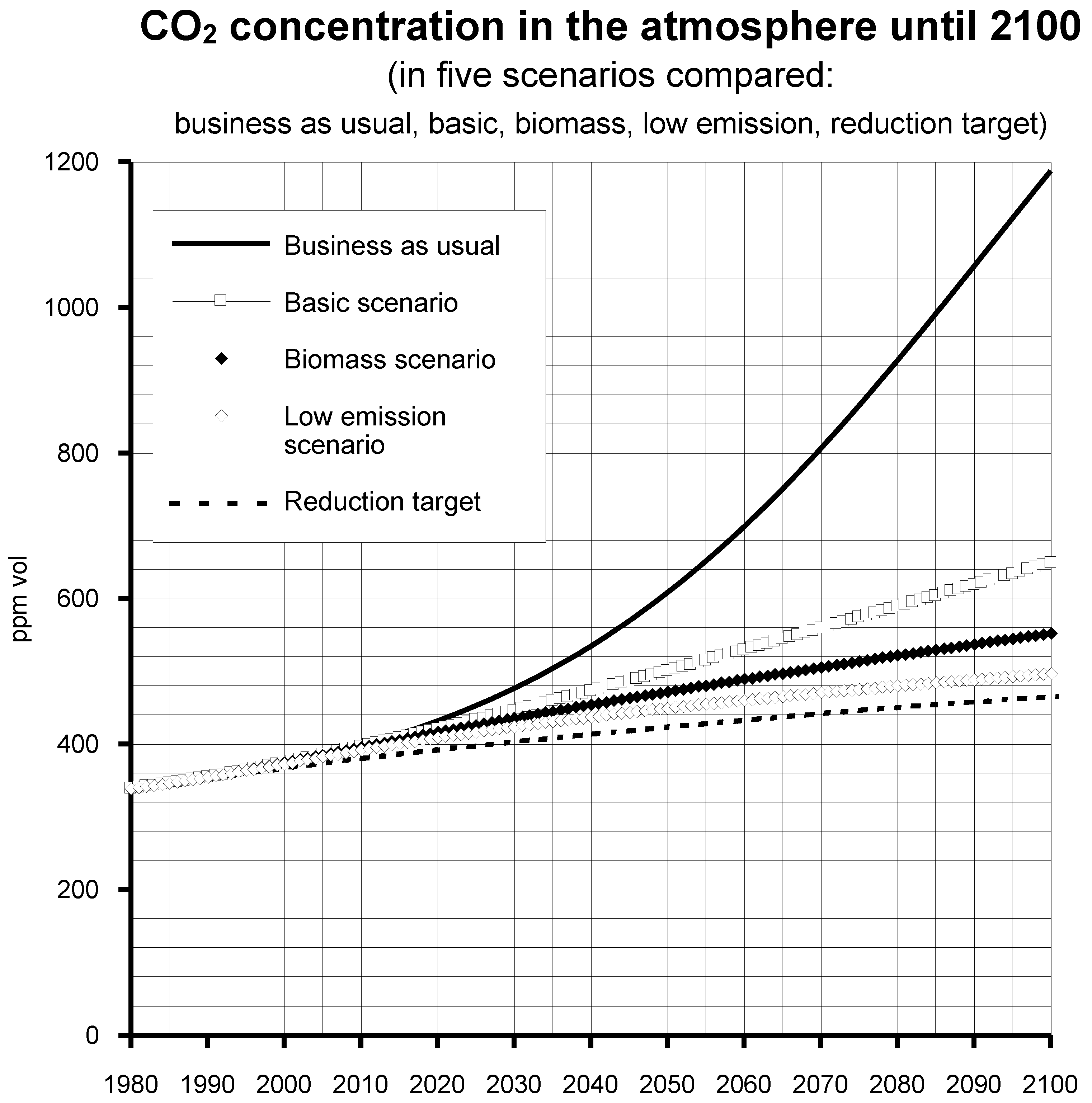
Table 2. Comparison of the CO2 reduction by 2100 achievable by different measures as quantitatively evaluated by CEBM scenarios (see Figure 11).
Mitigation Measure
(CEBM Scenario)
Atmospheric CO2 Content
in the Year 2100 in ppm
CO2 Reduction Compared
to the Trend Case for 2100
Trend = business as usual (+3%/a increase in emissions due to the increase in energy demand)approx. 1200-
Global maximum biomass use (with trend scenario: +3%/a)approx. 1000approx. 150
Reduction of the increase in emissions or energy demand from +3% to +1% (base scenario)approx. 650approx. 550
Combination of both methods (biomass scenario)approx. 550 approx. 650
Reduction target (−1%/a)approx. 450approx. 750
Publisher’s Note: MDPI stays neutral with regard to jurisdictional claims in published maps and institutional affiliations.

