Abstract
The paper presents a new approach to designing the stator of a multistage centrifugal pump, which has a simple structure, satisfactory operating parameters, and is easy to manufacture. The stator is distinguished by its lack of a classic diffuser part, with the shape of its crossover being similar to a segment of a spherical surface. This solution was patented in 1989, but to date it is not well known and practically not used. The paper attempts to identify the flow phenomena in such a stator and also to examine the impact of the design features of the stator on the pump’s operating parameters. Both experimental methods and numerical modelling were used in the research.
1. Introduction
Multistage centrifugal pumps constitute an important group of machines that are necessary for the functioning of such sectors of the economy as: energy; mining; heating; the chemical industry; water supply; etc. Regarding flow, a multistage pump is a series circuit connection of many sections (stages), consisting of, e.g., an impeller and a stator (Figure 1).
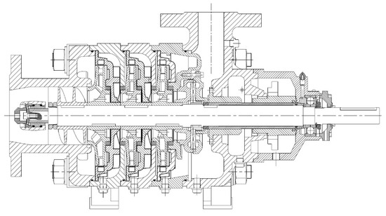
Figure 1.
Cross-section through a multistage centrifugal pump (http://www.pumps-hv.com/multistage_rotodynamic_pumps.php, (accessed on 20 May 2014).
Guide vanes are flow elements of multistage pumps which fulfill the following functions:
- Ensuring the assumed nominal flow rate, head, and hydraulic efficiency;
- Converting the kinetic energy of the liquid flowing out of the impeller into potential energy;
- Changing the direction and value of the fluid velocity from the impeller outlet to the direction and value of the velocity of the impeller inlet of the next pump’s stage, while at the same time ensuring minimal losses and the most even velocity field;
- Equalizing radial pressures acting on the impeller.
The theoretical characteristics of the discharge element can be determined by knowing that at the best efficiency point (BEP) of the momentum that is obtained from the impeller must be equal to the momentum in the stator. The graphical interpretation of the above dependence is shown in Figure 2. The intersection of the theoretical characteristics of the stator and the impeller determines the minimum hydraulic losses, i.e., the maximum hydraulic efficiency. Due to this, the position of the best efficiency point of the pump on the flow characteristic depends on the capacity of the stator, especially in the case of pumps with a relatively low value of kinematic specific speed [1].
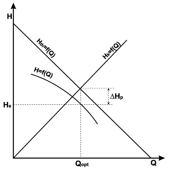
Figure 2.
Characteristics of the cooperation between the impeller and the stator: Hth = f(Q)—characteristics of the impeller, Hk = f(Q)—characteristics of the stator, H = f(Q)—actual characteristics of the pump (the author’s elaboration).
The basic elements of the stator with guide vanes (Figure 3):
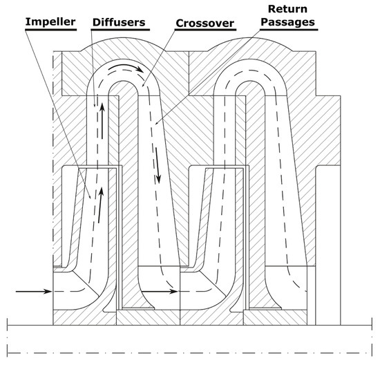
Figure 3.
Elements of a multistage pump stator [3].
- Diffusers—elements in which the kinetic energy of flowing liquid is converted into potential energy, with the efficiency of this transformation largely determining the hydraulic efficiency of the entire pump. The capacity of the diffusers affects the location of the best efficiency point on the flow characteristics [1].
- Crossover (term consistent with [2]; in book [3], the terms U-turn and “return channel” can be found, whereas in [1]—“annulus”.)—an element, the main task of which is to change the direction of the flow of fluid from centrifugal to centripetal. There are stators that have a crossover with vanes and also ones without them. Due to technological reasons, stators with a vaneless crossover are used more often. By using a crossover with vanes, an increase in efficiency of about 2 to 3% can be achieved.
- Return passages—elements, the task of which is to bring liquid to the inlet of the impeller of the next pump stage with the lowest possible hydraulic losses and the most even velocity field.
A review of the construction of the stators that are used in multistage pumps and the principles of their design can be found in books [1,2,3]. In addition, the results of research concerning the use of Computational Fluid Dynamics (CFD) in the design of stators, new ways of constructing stators, or the influence of their features on operating parameters are presented in studies [4,5,6,7,8,9]. Paper [10] provides a summary of the research carried out in recent years.
Stators with a crossover shaped as a spherical surface and without diffuser parts are an alternative solution to the design of guide vanes in small multistage pumps. Such stators are protected by patent [11] and are characterized by an extremely simple design (Figure 4) which translates into an uncomplicated production technology (the possibility of applying plastic forming methods) and thus a low production cost. Moreover, due to the fact that a “pseudo diffuser part” is formed between the impeller’s outlet surface and the internal surface of the crossover and the pump’s walls, hydraulic operating parameters are also satisfactory.
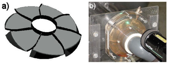
Figure 4.
A4 stator with a crossover shaped as a spherical surface; (a) 3D model; (b) stator installed in the model pump.
The current state of knowledge concerning stators with a crossover shaped as a spherical surface is insufficient and is mainly based on several papers [12,13]. These studies constitute the first attempt to describe research on improving the 25YS pump stage. The results of these works proved that such a method of shaping the crossover of a stator is beneficial in terms of energy (higher efficiency), technology, and the economy. The experience gained in this area led to the construction of a stator (with the designation of A4) which, in combination with a cast impeller, achieved the best operating parameters of the pump stage with regards to the area of research.
This paper presents the results of extensive research concerning the influence of the design features of a stator with a crossover shaped as a spherical surface on a pump’s operating parameters. As part of the carried-out work, flow phenomena in the channels of such a guide vanes were identified using both experimental and numerical methods. Thanks to this, it will be possible to design such stators in a rational way.
2. Research Object
The starting point for this research work was the model of the 25YS pump stage, which consists of a cast centrifugal impeller and an A4 stator that is made of metal sheet using a method of deep drawing. The basic geometric parameters of the impeller and the stator are shown in Figure 5 and Figure 6 and also in Table 1 and Table 2. Based on the above elements, a model pump was designed, and it constituted a single stage of a multistage pump (Figure 4b), which was then used in further tests on a test rig.
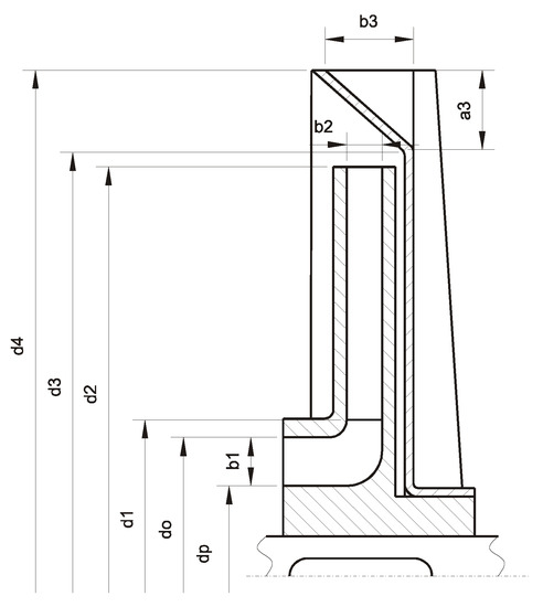
Figure 5.
Characteristic dimensions of the pump stage.
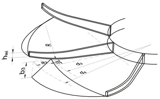
Figure 6.
Characteristic dimensions of the guide vanes with the crossover shaped as a spherical surface.

Table 1.
Characteristic dimensions of the impeller of the model pump (Figure 5).
3. Test Rig
The aim of the experimental research was to obtain the data that are necessary to prepare the numerical model and also to verify the obtained calculation results. The following scope of research was planned within the project:
- Measurements of the performance characteristics of the model pump stage, which aim to determine the basic curves of the pump stage (H = f(Q), P = f(Q), η = f(Q)) and the parameters of the best efficiency point (BEP) of the pump stage. Further tests and numerical calculations will be performed for the BEP determined in this way.
- Measurements of velocity distributions—measurements of the local velocity of fluids in the return channels of the stator using the LDA (Laser Doppler Anemometer) method are planned, the results of which will be used to verify the numerical model.
- Visualization tests that aim to obtain an image of the structure of the flow in the stator’s channels. Due to this, it will be possible to qualitatively verify the numerical results.
The tests were carried out on a test rig, the diagram of which is shown in Figure 7. The main element is a model pump (Figure 4b) which is fed from an open tank that has a volume of 0.3 m3. The measuring instruments are listed in Table 3.
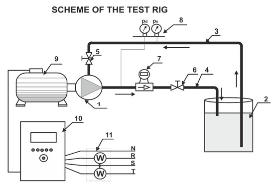
Figure 7.
Scheme of the test rig: 1—model pump; 2—open tank; 3—suction pipe; 4—discharge pipe; 5—shut-off valve; 6—regulating gate valve; 7—electromagnetic flow meter; 8—measuring manometers; 9—electric motor; 10—inverter; 11—measurement of electric power using wattmeters in the Aronna system.
Table 3.
List of instruments used in the measurements.
A DANTEC 60X laser anemometer was used to measure the velocity distributions [14]. The device is controlled by means of a computer and FLOware software. The technical data of the used anemometer are presented in Table 4. Measurements of velocity distributions were conducted on the crossover and in the return passage of the stator in the cross-sections shown in Figure 8.
Table 4.
Technical data of the DANTEC 60X laser anemometer.
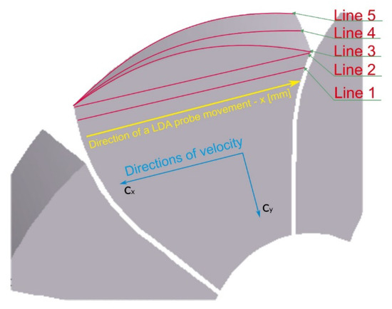
Figure 8.
Measurement cross-sections for the LDA method.
The “air bubble” method was used for the visualization tests. The diagram of supplying air to the flowing liquid is shown in Figure 9.
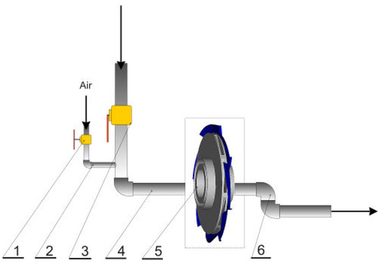
Figure 9.
Scheme of supplying air during the visualization tests: 1—air quantity control valve; 2—air supplying pipe; 3—shut-off valve; 4—suction pipe; 5—model pump; 6—discharge pipe.
The results of the measurements of the performance characteristics of the model pump stage are shown in Figure 10.
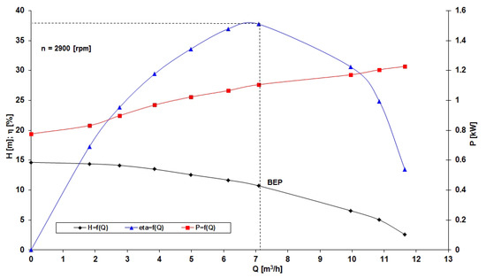
Figure 10.
Performance curves of the model pump.
4. Numerical Model
In order to accurately identify the flow phenomena in the flow channels of the stator with the crossover shaped as a spherical surface, numerical CFD flow simulations were performed using the Fluent 6.3 program (now included in ANSYS software). This software solves equations of conservation: mass (1) and momentum (2) (for x-axis) [1] using the Finite Volumes Method [15].
The flow in the stator can be treated as a periodically symmetric problem (assuming that each channel of the stator is made with the same accuracy), and therefore it is enough to model the flow in one passage to obtain information about the flow phenomena in the entire discharge element (Figure 11). Such a creation of the model significantly reduces the number of computational mesh elements and thus reduces the computing resources required by the computer. When creating the model, the following simplifying assumptions were made:
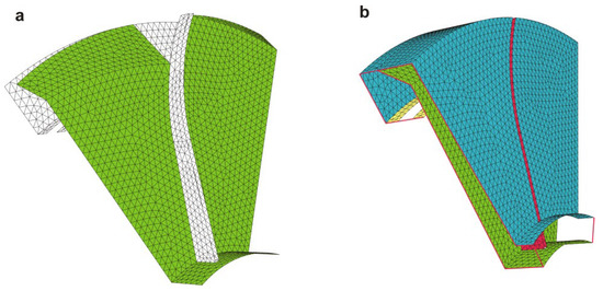
Figure 11.
Surfaces of the numerical model: (a) without the top wall of the body; (b) with the top wall of the body.
- The outlet from the impeller was treated as a continuous surface (the thickness of the impeller’s blades was omitted);
- The influence of the rotating surfaces of the impeller was omitted;
- A homogeneous velocity distribution on the impeller’s outlet surface was assumed.
The surfaces of the numerical model are shown in Figure 11.
The computational mesh was generated based on tetrahedral elements. The number of mesh elements was determined according to the Grid Independence Test as 400,000 elements. This in turn resulted in the value of parameter y+ < 30. The numerical velocity values at the impeller’s outlet (inlet to the model) were determined on the basis of the pump’s energy measurements and in accordance with the algorithm presented in Table 5. The boundary conditions imposed on the individual surfaces of the model are shown in Figure 12 and in Table 6.
Table 5.
Algorithm for determining the velocity components (cm3, cu3) on the impeller’s outlet [3].
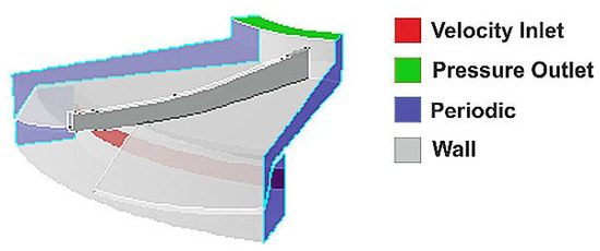
Figure 12.
Boundary conditions assumed for the model.
Table 6.
Boundary conditions and fluid properties used in the calculations.
In order to verify the results of the calculations, a comparison of the velocity distributions in the return channels of the stator with the crossover shaped as a spherical surface, those obtained using the LDA method and the numerical methods with the use of various models of turbulence, was carried out. Taking into account the calculation time, the number of iterations, the course of the convergence curve, and the guidelines included in the program documentation [15], the analysis of velocity distributions in the return channels of the stator were carried out for four combinations of turbulence models:
- Spalart-Allmaras;
- k-ε standard + the non-equilibrium near wall function;
- RNG k-ε + the non-equilibrium near wall function;
- Realizable k-ε + the non-equilibrium near wall function.
More details regarding the selected turbulence models (description, equations, and recommendations of application) can be found in [1,15]. The turbulence models listed above were used with a standard set of constants [15]. The analysis was performed in the measurement cross-sections according to Figure 8 for the velocity components cx and cy (Figure 8). The results are shown in Figure 13, Figure 14, Figure 15, Figure 16 and Figure 17.
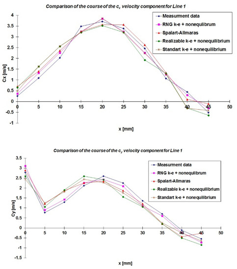
Figure 13.
Comparison of the course of the cx, cy velocity components for Line 1.
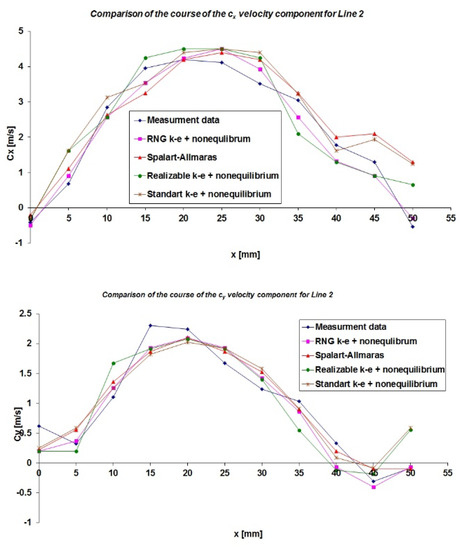
Figure 14.
Comparison of the course of the cx, cy velocity components for Line 2.
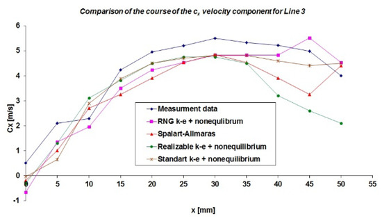
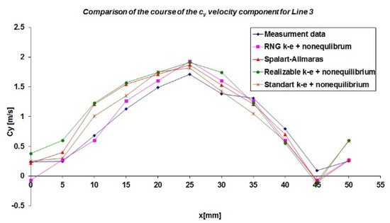
Figure 15.
Comparison of the course of the cx, cy velocity components for Line 3.
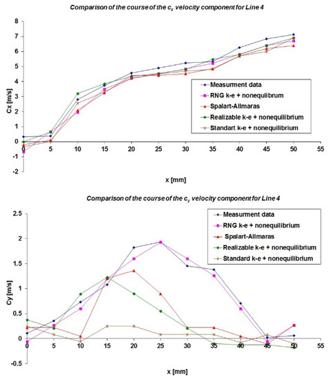
Figure 16.
Comparison of the course of the cx, cy velocity components for Line 4.
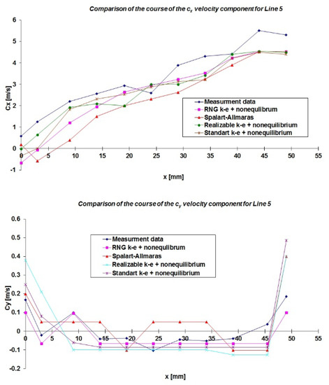
Figure 17.
Comparison of the course of the cx, cy velocity components for Line 5.
By analyzing the above graphs (Figure 13, Figure 14, Figure 15, Figure 16 and Figure 17), the following conclusions can be drawn:
- Good accordance between the velocity curves obtained using experimental and numerical methods was observed.
- Most of the calculation points were within 20% of the tolerance of the measured data.
- The greatest discrepancies in the numerical and measurement data occur in the vicinity of the wall; in the central flow region, the discrepancies are much smaller.
- The best agreement of the experimental and numerical results was obtained for the RNG k-ε + non-equilibrium near wall turbulence model.
For the selected turbulence model (RNG k-ε + non-equilibrium near wall model), the flow structure obtained using numerical calculations was compared with the results of the visualization tests (Figure 18). There are three areas that can be distinguished in the flow:
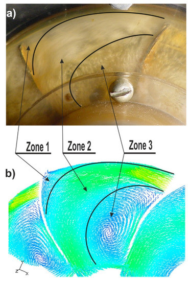
Figure 18.
The structure of flow in the return channels obtained: (a) from the experiment; (b) from the calculations.
- Zone 1—reduced velocity zone;
- Zone 2—mainstream flow;
- Zone 3—turbulence zone.
By analyzing Figure 18, it is possible to find a high convergence of the characteristic zones in the areas of experimental and computational flow, which additionally confirms the correctness of the adopted procedure for modeling the flow in the stator with the crossover shaped as a spherical surface. For further calculations, the RNG k-ε turbulence model and the non-equilibrium near wall model were selected.
5. Numerical Research and Results
Using the verified numerical model, a numerical analysis of the influence of the geometrical features of the stator with the crossover shaped as a spherical surface on the parameters of its work was performed. The A4 stator (base variant) was adopted as the starting variant for the numerical tests. In the course of the calculations, the tested parameter was changed—with the invariability of other geometric quantities being kept. The study analyzed the influence of the following quantities (Figure 6):
- The stator’s inlet diameter d3;
- The number of the stator’s vanes zk;
- The radius of the vane R;
- Dimensions of the inlet cross-section of the stator: a3 and b3;
- Inflection angle of a vane εk.
The main function of the stator in a multistage pump is to supply liquid to the inlet of the impeller of the next stage with the velocity field as even as possible and with minimal losses. Therefore, two parameters were adopted as the criteria for evaluating alternative solutions:
- The efficiency of the stator (3), defined as the ratio of the total outlet pressure to the total inlet pressure. The total pressure is defined as the sum of the static and dynamic pressures (4). This parameter determines the energy efficiency of the discharge element:
- Velocity compensation factor (5), defined as the ratio of the velocity component (perpendicular to the outlet) to the total velocity. This parameter determines the working conditions of the next stage’s impeller. The aim is for this coefficient to be close to one:
For the operation of the entire multistage pump, both criteria have the same weight, and therefore the objective function is defined as (6):
where:
x1 = η,
x2 = kc
In Figure 19, the velocity distribution and static pressure distribution are presented for the A4 basic stator as a reference point.
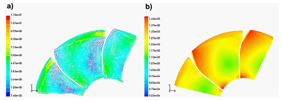
Figure 19.
The field of: (a) velocity [m/s]; (b) static pressure [Pa] in the channels of the guide vanes for the basic variant (stator A4).
5.1. The Effect of the Stator’s Inlet Diameter
Four variants of the stator (with different ratios of diameters d2/d3) were tested. The results are presented in Table 7. The text highlighted in gray shows the results for the basic A4 stator.
Table 7.
The effect of the inlet diameter of the guide vanes.
The objective function reaches its maximum at the ratio of diameters d2/d3 = 1. Such a result seems very intuitive because it is the impeller’s outlet surface, together with the surfaces of the crossover and the pump’s body walls, that form the “pseudo diffusers.” The velocity and pressure distributions for the d2/d3 = 1 variant are presented in Figure 20. In this case, the more uniform pressure distribution can be observed compared with the basic variant (Figure 19).
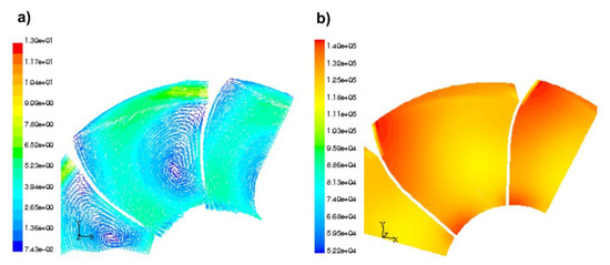
Figure 20.
The field of: (a)—velocity [m/s]; (b)—static pressure [Pa] in the channels of the guide vanes for the d2/d3 = 1 variant.
5.2. The Effect of the Number of Guide Vanes
Five variants of the stator with a different number of return vanes zk were tested. The results are presented in Table 8. The text highlighted in gray shows the results for the basic A4 stator.
Table 8.
The effect of the number of guide vanes.
The objective function reaches its maximum for the number of guide vanes zk = 11, which is consistent with the data presented in [1]. The use of a larger number of vanes results in narrower passages and a better equalization of the velocity at the impeller’s inlet of the next stage (kc increase), as well as a more uniform pressure distribution in the return channels when compared to the basic stator (Figure 19). When the flow channels are narrowed too much (zk = 12), the efficiency drops due to an increase in hydraulic losses. The velocity and pressure distributions for the zk = 11 variant are presented in Figure 21.
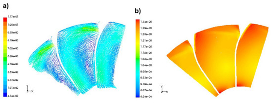
Figure 21.
The field of: (a) velocity [m/s]; (b) static pressure [Pa] in the channels of the guide vanes for variant zk = 11.
5.3. The Effect of the Dimensions of the Inlet Cross-Section of the Crossover
Five variants of the stator, with different dimensions of the inlet cross-section a3 and b3, were tested, while at the same time maintaining the constant area of the inlet cross-section A3 = 40.5 mm2 (A3 = 0.5 a3b3). The results are presented in Table 9. The text highlighted in gray shows the results for the basic A4 stator.
Table 9.
The effect of the dimensions of the inlet cross-section of the crossover.
The objective function reaches its maximum for the ratio of the inlet cross-section of the crossover of a3/b3 = 1.25. When the number of guide vanes is changed, the inlet area of a single channel also changes, and therefore the optimal dimensions of the inlet cross-section of the stator may also be related to the assumed number of guide vanes. It is clear that more favorable results are obtained when a3 is greater than b3. The velocity and pressure distributions for the variant of a3/b3 = 1.25 (a3 = 10.125 mm; b3 = 8 mm) are presented in Figure 22 and are slightly more uniform when compared to the basic variant (Figure 19).
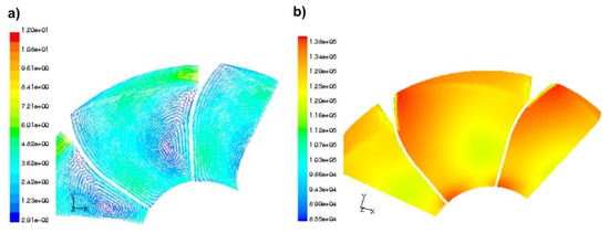
Figure 22.
The field of: (a) velocity [m/s]; (b) static pressure [Pa] in the channels of the guide vanes for the variant of a3/b3 = 1.25.
5.4. The Effect of the Radius of a Guide Vane
Five variants of the stator with different dimensions of the radius of return vane R were tested. The results are presented in Table 10. The text highlighted in gray shows the results for the basic A4 stator.
Table 10.
The effect of the radius of a return vane.
The objective function reaches its maximum for the value of the radius of a return vane R = 30 mm. The radius is a parameter that affects efficiency to a very small extent, but it does have quite a significant impact on the smoothing of the velocity field in front of the inlet to the next stage’s impeller. The velocity and pressure distributions for the R = 30 mm variant are presented in Figure 23 and are similar to the basic variant (Figure 19).
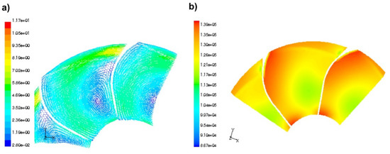
Figure 23.
The field of: (a) velocity [m/s]; (b) static pressure [Pa] in the channels of the guide vanes for the radius R = 30 mm.
5.5. The Effect of the Inclination Angle of a Return Vane
Seven variants of the stator with different angles of the inclination of the rectilinear section of a return vane εk were tested. The results are presented in Table 11. The text highlighted in gray shows the results for the basic A4 stator.
Table 11.
The effect of the angle at the end of a return guide vane.
The objective function reaches its maximum for a return vane angle at the outlet of εk = 25° which results in an outlet angle of α6 = 115°. According to the recommendations that are available in the literature, angle εk should be assumed within the range from 5° to 8° [1]. However, in the case of a stator with a crossover shaped as a spherical surface, such a large value of the optimal angle εk (25 degrees) results from a much greater swirl of the liquid in the return passages, which must be compensated by a much greater bending of the vane. The velocity and pressure distributions for the variant of εk = 25° are presented in Figure 24 and are similar to the basic variant (Figure 19).
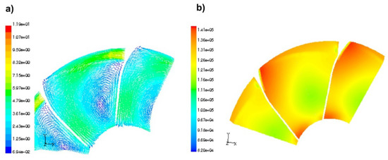
Figure 24.
The field of: (a) velocity [m/s]; (b) static pressure [Pa] in the channels of the guide vanes for εk = 25°.
6. Summary
Guide vanes with a crossover shaped as a spherical surface are an interesting alternative to the design of the stators that are used in multistage pumps. The study investigated the influence of the geometrical parameters of such a stator on the operating parameters of the pump stage. CFD modelling was applied as the main research method. The proposed numerical model was verified using the results of experimental tests. The scope of the tests included energy curve measurements, measurements of velocity distributions using a laser doppler anemometer, and performing flow visualization. The discrepancies of the results between the experimental data and those obtained from the numerical CFD calculations, depending on the used turbulence model, were on average 20% in the case of velocity (the maximum discrepancies occurred near the wall and on the boundary between Zones 1, 2, and 3—Figure 18).
For further calculations, the RNG k-ε turbulence model and the non-equilibrium near wall model were selected. This combination ensured: good convergence of the calculation results with those obtained from the experimental tests; good stability of the conducted calculations; and a relatively small number of required iterations.
Numerical studies of the influence of particular geometrical dimensions of the stator on the parameters of its work were carried out. The analysis of the graphical and numerical results of the calculations enabled the nature of the flow in the stator with the crossover shaped as a spherical surface to be analyzed and the knowledge concerning such discharge elements to be deepened and systematized.
On the basis of the performed calculations, the following general conclusions were formulated:
- The verified numerical 3D model of the flow in the stator with the crossover shaped as a spherical surface enables a description of the flow phenomena in such stators, and also in geometrically similar stators, to be obtained.
- The obtained numerical results deepen the current state of knowledge regarding the flow phenomena in the discussed discharged element, thanks to which it is easier to rationally shape the flow passages of such stators.
- By using CFD programs, the shape of a stator can be rationalized by obtaining information about the energy changes that take place in it.
- Thanks to numerical tests, the number of necessary experimental tests can be significantly reduced and thus also the cost of experimental research.
- Conducting numerical CFD studies allows for the observation of phenomena in any place of the geometry of the considered flow elements which is not always possible in the case of real experimental studies.
- Two parameters have the largest influence on the pump’s operating conditions: the number of vanes and the stator’s inlet diameter.
Author Contributions
Conceptualization, J.S.; Methodology, J.S.; Software, W.L.; Formal analysis, P.S.; Investigation, J.S.; Resources, W.L.; Data curation, P.S.; Writing—original draft, J.S.; Writing—review & editing, P.S. and W.L.; Visualization, W.L. All authors have read and agreed to the published version of the manuscript.
Funding
This research received no external funding.
Data Availability Statement
The data presented in this study are available on request from the corresponding author.
Conflicts of Interest
The authors declare no conflict of interest.
Nomenclature
| a3 | width of the inlet cross-section of the stator with the crossover shaped as a spherical surface | [m] |
| b2 | width of the impeller’s passage at the outlet | [m] |
| b3 | hight of the inlet cross-section of the stator with the crossover shaped as a spherical surface | [m] |
| c3 | real absolute velocity at the impeller outlet | [m/s] |
| cm3, cu3 | components of the absolute velocity at the impeller outlet | [m/s] |
| co | total velocity at the outlet of the model (impeller inlet of the next stage) | [m/s] |
| cx, cy | components of velocity in the Cartesian coordinate system | [m/s] |
| cz | velocity component perpendicular to the outlet of the model (inlet cross-section of the impeller next stage) | [m/s] |
| d2 | outer diameter of the impeller | [m] |
| d3 | inlet diameter of the stator | [m] |
| d4 | outer diameter of the diffuser | [m] |
| H | head | [m] |
| hwi | height of the return vanes at the inlet | [m] |
| Ix,Iy | turbulence intensities corresponding to velocity cx, cy | [%] |
| k | turbulent kinetic energy | [m2/s2] |
| kc | velocity compensation factor | ---- |
| n | rotation speed | [rpm] |
| nsQ | kinematic specific speed | [rpm] |
| p | the Pfleiderer’s slip factor | ---- |
| pt | total pressure | [Pa] |
| pti | total pressure at the model inlet | [Pa] |
| pto | total pressure at the model outlet | [Pa] |
| ps | static pressure | [Pa] |
| pd | dynamic pressure | [Pa] |
| Q | flow rate | [m3/s] |
| s2 | thickness of the impeller blade at the outlet | [m] |
| s3 | thickness of the guide vane at the inlet | [m] |
| w | relative velocity | [m/s] |
| t2 | pitch at the impeller outlet | [m] |
| y+ | dimensionless distance from the wall | ---- |
| z | number of impeller blades | ---- |
| zk | number of guide vanes | ---- |
| α3 | angle of absolute velocity at the impeller outlet | [°] |
| β2 | outlet angle of the impeller blades | [°] |
| ε | turbulent dissipation energy | [m2/s2] |
| εk | angle of inflection of a return vanes | [°] |
| μ | viscosity | [Pas] |
| η | efficiency | ---- |
| ρ | desity | [kg/m3] |
| Φ | objective function | ---- |
| ϕ2 | coefficient of the constriction at an impeller outlet | ---- |
References
- Gulich, J.F. Centrifugal Pumps; Springer: Berlin, Germany, 2008. [Google Scholar]
- Lobanoff, V.S.; Ross, R.R. Centrifugal Pumps. In Design and Application; Gulf Publishing Company: Houston, TX, USA, 1992. [Google Scholar]
- Lazarkiewicz, S.; Troskolański, A. Impeller Pumps; WNT: Warsaw, Poland, 1965. [Google Scholar]
- Kawashima, D.; Kanemoto, T.; Sakoda, K.; Wada, A.; Hara, T. Matching Diffuser Vane with Return Vane Installed in Multistage Centrifugal Pump. Int. J. Fluid Mach. Syst. 2008, 1, 91. [Google Scholar] [CrossRef]
- Miyano, M.; Kanemoto, T.; Kawashima, D.; Wada, A.; Hara, T.; Sakoda, K. Return Vane Installed in Multistage Centrifugal Pump. Int. J. Fluid Mach. Syst. 2008, 1, 57–63. [Google Scholar] [CrossRef]
- La Roche-Carrier, N.; Ngoma, G.; Ghie, W. Numerical Investigation of a First Stage of a Multistage Centrifugal Pump: Impeller, Diffuser with Return Vanes, and Casing. ISRN Mech. Eng. 2013, 2013, 578072. [Google Scholar] [CrossRef]
- Zhang, Q.; Shi, W.; Xu, Y.; Gao, X.; Wang, C.; Lu, W.; Ma, D. A New Proposed Return Guide Vane for Compact Multistage Centrifugal Pumps. Int. J. Rotating Mach. 2013, 2013, 683713. [Google Scholar] [CrossRef]
- Lugovayaa, S.; Olshtynskyb, P.; Rudenkoc, A.; Tverdokhleb, I. Revisited Designing of Intermediate Stage Guide Vane of Centrifugal Pump. Procedia Eng. 2012, 39, 223–230. [Google Scholar] [CrossRef]
- Varchola, M.; Hlbočan, P. The Influence of the Radial Diffuser Geometry on the Position of Best Efficiency Point of the Multistage Pump. AIP Conf. Proc. 1608, 257, 2014. [Google Scholar] [CrossRef]
- Rodea, B.R.; Khare, R. A review on development in design of multistage centrifugal pump. Adv. Comput. Des. 2021, 6, 43–53. [Google Scholar] [CrossRef]
- Misiewicz, W.; Trasa, K.; Plutecki, J. Kierownica Wielostopniowej Pompy Wirowej. Patent PL 159402 B1, 31 December 1992. [Google Scholar]
- Plutecki, P.; Skrzypacz, J. The shape optimization of a small diffuser ring with spherical surface, W: Mechanical engineering. In Proceedings of the Presented Papers, Bratislava, Slovakia, 22 November 2001; Slovenska Technicka Univerzita: Bratislava, Slovakia, 2001; pp. 145–150. [Google Scholar]
- Plutecki, J.; Skrzypacz, J. CDF simulations of 3D flow in a pump stator with a spherical surface. World Pumps 2003, 443, 28–31. [Google Scholar]
- FLOware. “User’s Guide 60X FiberFlow”, “User’s Guide FLOware”; Dantec Mesurement Technology A/S: Ballerup, Denmark, 1992. [Google Scholar]
- Fluent. Fluent–“User’s Guide”, “Tutorial Guide”; Fluent Incorporated: Lebanon, NH, USA, 1993. [Google Scholar]
Publisher’s Note: MDPI stays neutral with regard to jurisdictional claims in published maps and institutional affiliations. |
© 2022 by the authors. Licensee MDPI, Basel, Switzerland. This article is an open access article distributed under the terms and conditions of the Creative Commons Attribution (CC BY) license (https://creativecommons.org/licenses/by/4.0/).