A Study on Magnetotelluric Characteristics of Magmatic Geothermal Systems

Abstract

The Magnetotelluric (MT) method is a widely used and effective method of exploring geothermal resources because it can reveal geological information at a great depth and is cost effective. In order to further improve the reliability and rationality of MT data interpretation, MT responses for a typical hydrothermal system and a hot dry rock (HDR) and partial melting system are investigated by a finite-element (FE) forward modeling approach based on unstructured tetrahedral grids that can handle with complex-shaped geothermal systems. These two geothermal models, designed by the 3ds Max software, are comprised of a clay cap, a reservoir, and a heat source, and are discretized into tetrahedral elements by TetGen software. The results show that the apparent resistivities at the broadband of frequencies are mainly affected by the shallow low-resistivity clay cap due to its strong shielding effects, and the induction arrows effectively reflect the boundary of the clay cap. The conductive heat-conducting path and heat source (1 S/m) considered in the models of the HDR and partial melting system could cause significant changes in the apparent resistivities and induction arrows at low frequencies. It suggests that in addition to the apparent resistivities, the induction arrows should be taken into consideration in MT data processing and inversion for better lateral resolution when exploring geothermal resources.

1. Introduction

Geothermal resources are viewed as systems storing heat in rocks and fluids within the Earth. Depending on whether the system is related to the emplacement of magma or not, it can be divided into two categories, namely magmatic geothermal systems and non-volcanic resources [1]. Magmatic geothermal systems can be subdivided into hydrothermal systems as well as HDR and partial-melt systems. For an ideal hydrothermal system, a conceptual model is comprised of a heat source, a reservoir, and a rock cap [2,3]. The heat source is always represented by a magma chamber or intrusive bodies. The reservoir mainly consists of fractured host rocks filled with high-concentration fluids, and also acts as a heat conduction path. The rock cap is made up of impermeable clay alteration layers, which are generated by prolonged reactions between overlying rocks and thermal fluids [1]. For a typical HDR and partial melting system the reservoir mainly refers to shallow HDRs. The heat is transported from the deep heat source to the reservoir via the instantaneous heat conductive process, as well as vertically elongated faults [4,5].

Magmatic geothermal systems always possess low resistivities compared with host rocks [6,7]. The underlying reasons for this phenomenon include: (1) the heat source has a high temperature, sometimes is partially melted, and therefore it is very conductive; (2) the cap rocks contain electrically conductive smectite and illite; (3) the heat source and reservoir are well-connected by fractures and faults filled of hot, saline, and electrically conductive fluids. Hence, electromagnetic (EM) methods are recognized as one of the geophysical tools that can be used to explore magmatic geothermal systems effectively. There are several EM techniques that have been used for exploring geothermal resources, such as Magnetotelluric (MT) [8,9], frequency-domain controlled-source EM methods [10], and time-domain EM methods [11]. Among these methods, MT is the most popular one because it has a large investigation depth and is more cost effective compared with controlled-source EM methods. In addition, MT data are easily contaminated by cultural noises, especially in the induction arrows. The development of data-processing techniques, such as remote reference and robust estimation methods [12,13], makes MT applications in cultural-noise environments possible.

There have been plenty of references to employing the MT technique to delineate three-dimensional (3D) structures of magma geothermal systems. For example, Newman et al. developed a 3D resistivity model with a full 3D inversion of an MT dataset and then confirmed that faulting strongly controls geothermal fluid production at Coso, CA, USA [8]. Ryan et al. constructed a 3D conceptual model of the Montserrat geothermal system based on MT as well as P wave seismic tomography and found that two intersectional faults play a crucial role in forming the geothermal system [14]. Samrock et al. obtained the typical electrical conductivity distribution of a high-enthalpy geothermal system from 3D inversions of MT data collected at the Aluto-Langano geothermal field, Ethiopia [15]. Peacock et al. established the 3D electrical-resistivity model of the hydrothermal system in Long Valley Caldera, CA, USA, and then well characterized the heat reservoir and heat source [7]. Gao et al. defined the magma geothermal system beneath the Gonghe Basin, Northeast Tibetan Plateau based on the 3D inversion results of a broadband MT dataset and inferred that the heat source is the partially melted granite in the middle crust [4]. Zhou et al. delineated the electrical-conductivity geothermal structure of the Yanggao geothermal field in Datong Basin, northern China using 3D MT inversion results [5]. In addition, the MT technique is also used to monitor subsurface fracture connectivity and fluid distribution when injecting conductive fluid into HDRs for enhanced geothermal systems [6,16]. Apparent resistivity and phase tensor are employed in order to effectively reflect the transient variations in the subsurface.

As stated above, MT plays an important role in delineating structures of geothermal systems. In order to further improve the reliability and rationality of MT data interpretation, this study is dedicated to investigating characteristics of apparent resistivity and induction arrows for a typical hydrothermal system and an HDR and partial melting system. A vector FE method using unstructured tetrahedral grids is chosen as the numerical method due to its capability of dealing with complex shapes of geothermal systems.

2. Methodology

This section will present the method of FE analysis used to calculate electric and magnetic fields, and the method of evaluating MT responses. The whole flowchart of this study is shown in Figure 1.

2.1. FE Method

With a time-dependence of $e^{i\omega t}$, Faraday’s and Ampère’s laws in a source-free region, and in the quasi-static regime, are written as

$$\nabla \times \mathbf{E}+i\omega \mu \mathbf{H}=0,$$

(1)

and

$$\nabla \times \mathbf{H}-\sigma \mathbf{E}=0,$$

(2)

where E and H denote the electric field and magnetic field, respectively. ω is the angular frequency and is defined by 2πf, with f being frequency. μ and σ are magnetic permeability and conductivity, respectively. Here, μ is set to the magnetic permeability of free space μ₀. Based on these two equations the Helmholtz equation for the electric field can be obtained:

$$\nabla \times \nabla \times \mathbf{E}+i\omega {\mu }_0\sigma \mathbf{E}=0.$$

(3)

Equation (3) is the governing equation for the vector FE method in this study. Considering that 3D magnetotellurics forward modeling based on FE methods and unstructured tetrahedral mesh are well developed [17,18], we present concise FE formulations here. For tetrahedral elements, the approximated electric field $\tilde{\mathbf{E}}$ in element e is expressed as

$$\tilde{\mathbf{E}}={\displaystyle \sum _{j=1}^6{\mathbf{N}}_j{E}_j^e},$$

(4)

where ${\mathbf{N}}_j$ and $E_j^e$ are the vector basis function and the approximated electric field corresponding to the jth edge, respectively. The residual $\mathbf{r}$ of Equation (3) is written as

$$\mathbf{r}=\nabla \times \nabla \times \tilde{\mathbf{E}}+i\omega {\mu }_0\sigma \tilde{\mathbf{E}}.$$

(5)

Based on the Galerkin method [19], multiplying the residual by the jth vector basis function, integrating over the computational domain $\mathsf{\Omega }$, and equating to zero leads to the following equation:

$${\displaystyle {\int }_{\mathsf{\Omega }}{\mathbf{N}}_j}\cdot \left(\nabla \times \nabla \times \tilde{\mathbf{E}}+i\omega {\mu }_0\sigma \tilde{\mathbf{E}}\right)d\mathsf{\Omega }=0.$$

(6)

Integrating by parts the first term on the left-hand side and setting the surface integrals to zero [20], equation 6 can be rewritten as

$${\displaystyle {\int }_{\mathsf{\Omega }}\left(\nabla \times {\mathbf{N}}_j\right)\cdot \left(\nabla \times \tilde{\mathbf{E}}\right)}d\mathsf{\Omega }+{\displaystyle {\int }_{\mathsf{\Omega }}i\omega {\mu }_0\sigma {\mathbf{N}}_j\cdot \tilde{\mathbf{E}}}d\mathsf{\Omega }=0.$$

(7)

Substituting Equation (4) into Equation (7), we obtain:

$${\displaystyle \sum _{e=1}^N\left({\displaystyle \sum _{j=1}^6{E}_j^e}{\mathbf{A}}_{ij}^e+i\omega {\mu }_0{\sigma }_e{\displaystyle \sum _{j=1}^6{E}_j^e{\mathbf{B}}_{ij}^e}\right)}=0,$$

(8)

where ${\mathbf{A}}_{ij}^e={\displaystyle {\int }_{{\mathsf{\Omega }}_e}\left(\nabla \times {\mathbf{N}}_i\right)\cdot \left(\nabla \times {\mathbf{N}}_j\right)}d{\mathsf{\Omega }}_e$, ${\mathbf{B}}_{ij}^e={\displaystyle {\int }_{{\mathsf{\Omega }}_e}{\mathbf{N}}_i\cdot {\mathbf{N}}_j}d{\mathsf{\Omega }}_e$, $i=1,\dots ,6$, N is the total number of tetrahedral elements. Equation (8) can be represented as the linear system of equations:

$$\left(\mathbf{A}+\mathbf{B}\right)\mathbf{x}=\mathbf{S},$$

(9)

where A and B are M × M matrices, and x and S are vectors of size M. M is the total number for tetrahedral edges and is also the number of degrees of freedom. x consists of the electric field along tetrahedral edges. Following the method used by Farquharson et al., Dirichlet boundary conditions are implemented by modifying matrices A and B, as well as the right-hand side S [20]. The elements of the right-hand side S are non-zero only for the edges located on the computational boundaries. Here the one-dimensional forward modeling method of Weaver [21] is used to calculate boundary electric field values.

Equation (9) is solved by the open-source direct solver MUMPS [22]. After obtaining x, the electric field $\tilde{\mathbf{E}}$ and magnetic field ${\tilde{\mathbf{H}}}^e$ at the observation point (x, y, z) located in the tetrahedral element e are evaluated by Equation (4) and the following equation:

$${\tilde{\mathbf{H}}}^e\left(x,y,z\right)=-\frac{1}{i\omega {\mu }_0}{\displaystyle \sum _{j=1}^6\nabla \times {\mathbf{N}}_j\left(x,y,z\right)E_j^e},$$

(10)

2.2. MT Responses

The impedance tensor Z is a basic MT response and describes the relationship between the horizontal components of the electric field and magnetic field. Z is complex-valued, and frequency dependent. In theoretical studies, Z is calculated from numerical EM responses [13,23]:

$$\left[\begin{array}{cc}{Z}_{xx}& Z_{xy}\\ Z_{yx}& Z_{yy}\end{array}\right]=\left[\begin{array}{cc}{\tilde{E}}_{x1}& {\tilde{E}}_{x2}\\ {\tilde{E}}_{y1}& {\tilde{E}}_{y2}\end{array}\right]{\left[\begin{array}{cc}{\tilde{H}}_{x1}& {\tilde{H}}_{x2}\\ {\tilde{H}}_{y1}& {\tilde{H}}_{y2}\end{array}\right]}^{-1},$$

(11)

where the subscripts x and y denote the x and y components of the electric field and magnetic field, respectively; the subscripts 1 and 2 indicate the forward EM responses under the E-x and E-y modes, respectively. The apparent resistivity can be calculated from the impedance tensor, namely

$$\begin{array}{cc}{\rho }_{kj}=\frac{1}{\omega {\mu }_0}{\left|Z_{kj}\right|}^2& \left(k=x,y;j=x,y\right)\end{array}.$$

(12)

Another basic MT response is the tipper transfer function T, which describes the relationship between the vertical and horizontal components of the magnetic field. T is also complex-valued and is defined by [13,24]

$$\left[\begin{array}{cc}{T}_x& T_y\end{array}\right]=\left[\begin{array}{cc}{\tilde{H}}_{z1}& {\tilde{H}}_{z2}\end{array}\right]{\left[\begin{array}{cc}{\tilde{H}}_{x1}& {\tilde{H}}_{x2}\\ {\tilde{H}}_{y1}& {\tilde{H}}_{y2}\end{array}\right]}^{-1},$$

(13)

where the subscripts are the same as Equation (11). The induction arrow, I, is always used to display the tipper, which can be constructed using the real parts of $T_x$ and $T_y$:

$$\mathbf{I}=\mathrm{Re}\left(T_x\right)\mathbf{x}+\mathrm{Re}\left(T_y\right)\mathbf{y}.$$

(14)

where x and y are the unit vectors along the x- and y-directions. Here we use the Wiese-convention [25], namely the direction of I is away from the conductive zone.

3. Results and Discussion

In this section, we will first test the FE method developed by ourselves, and then employ it to investigate the characteristics of apparent resistivity and induction arrows for models representing a typical hydrothermal system and an HDR and partial melting system.

3.1. FE Method Testing

The 3D FE forward modeling solver is tested by numerical solutions of the mesh-free method of Long and Farquharson [23]. The mesh-free method uses only a cloud of unconnected points to obtain numerical solutions throughout a computational domain, it is also termed a radial-basis-function-based finite difference. The geoelectric model used in the test is the COMMEMI 3D-1A model, which is first reported by Zhdanov et al. [26]. For this model, a conductive block is embedded in a half-space. The resistivities are 0.5 and 100 Ωm for the block and half-space, respectively. The block is 1 × 2 × 2 km³ in the x-, y-, and z-directions (Figure 2a). There are two survey lines arranged along the x- and y-directions. Each line has 61 stations with 100 m intervals (Figure 2b). The computational domain is set to 100 × 100 × 100 km³. The central domain of the tetrahedral mesh generated by TetGen 1.5.1 [27] is shown in Figure 2c,d.

Figure 3 shows the apparent resistivity curves for the COMMEMI 3D-1A model. Here the frequency is set to 0.1 Hz. As shown in Figure 3, the curves for both ρ_xy and ρ_yx calculated by the FE and the mesh-free methods are in good agreement with each other. The apparent resistivity data calculated by the FE method are shown in

Table 1. The apparent resistivities calculated by the FE method for the COMMEMI 3D-1A model. The frequency was set to 0.1 Hz. The apparent resistivity unit is Ωm.

x (m)	ρxy	ρyx	y (m)	ρxy	ρyx
0	1.64	0.99	0	1.64	0.99
200	3.52	1.07	200	1.66	1.04
400	21.30	1.71	400	1.73	1.26
600	89.12	4.52	600	1.96	2.69
800	134.51	11.58	800	2.94	12.89
1000	144.93	22.14	1000	6.99	80.97
1200	144.72	33.94	1200	19.73	184.31
1400	141.53	45.39	1400	38.49	204.47
1600	137.76	55.58	1600	55.71	192.97
1800	134.07	64.25	1800	68.50	177.67
2000	130.72	71.54	2000	77.71	164.69
2200	127.78	77.64	2200	84.25	154.46
2400	125.28	82.63	2400	89.17	146.63
2600	123.12	86.72	2600	92.70	140.53
2800	121.30	90.21	2800	95.39	135.57
3000	119.83	93.13	3000	97.44	131.56

. Figure 4 shows the induction arrow for the COMMEMI 3D-1A model, and the corresponding data are shown in

Table 2. The real parts of the tipper transfer function calculated by the FE method for the COMMEMI 3D-1A model. The y-coordinate is 0 m.

x (m)	Re (Tx)				Re (Ty)
	0.1 Hz	1 Hz	10 Hz	100 Hz	0.1 Hz	1 Hz	10 Hz	100 Hz
0	−9.70 × 10−5	−1.64 × 10−4	1.00 × 10−4	−1.88 × 10−5	−1.67 × 10−4	8.21 × 10−4	−1.30 × 10−4	2.68 × 10−5
200	1.69 × 10−2	9.02 × 10−2	7.53 × 10−2	2.04 × 10−2	−2.33 × 10−4	8.37 × 10−4	2.34 × 10−4	5.33 × 10−4
400	3.04 × 10−2	1.73 × 10−1	1.87 × 10−1	6.64 × 10−2	−3.12 × 10−4	7.82 × 10−4	4.69 × 10−4	−4.27 × 10−5
600	3.57 × 10−2	2.15 × 10−1	2.84 × 10−1	1.01 × 10−1	−3.80 × 10−4	6.73 × 10−4	5.80 × 10−4	−7.65 × 10−4
800	3.41 × 10−2	2.05 × 10−1	2.84 × 10−1	5.55 × 10−2	−3.92 × 10−4	6.47 × 10−4	7.16 × 10−4	−4.10 × 10−4
1000	3.04 × 10−2	1.76 × 10−1	2.35 × 10−1	1.14 × 10−2	−3.99 × 10−4	6.04 × 10−4	6.66 × 10−4	−2.03 × 10−4
1200	2.66 × 10−2	1.46 × 10−1	1.81 × 10−1	−8.19 × 10−3	−3.95 × 10−4	5.61 × 10−4	6.61 × 10−4	2.78 × 10−4
1400	2.32 × 10−2	1.20 × 10−1	1.36 × 10−1	−1.44 × 10−2	−4.38 × 10−4	3.79 × 10−4	2.16 × 10−4	−8.86 × 10−4
1600	2.02 × 10−2	9.87 × 10−2	1.02 × 10−1	−1.47 × 10−2	−4.07 × 10−4	4.20 × 10−4	5.05 × 10−4	1.31 × 10−4
1800	1.77 × 10−2	8.19 × 10−2	7.64 × 10−2	−1.22 × 10−2	−3.98 × 10−4	4.17 × 10−4	6.30 × 10−4	4.10 × 10−4
2000	1.56 × 10−2	6.84 × 10−2	5.68 × 10−2	−1.03 × 10−2	−4.05 × 10−4	3.68 × 10−4	5.54 × 10−4	8.99 × 10−5
2200	1.38 × 10−2	5.76 × 10−2	4.21 × 10−2	−8.63 × 10−3	−4.23 × 10−4	2.94 × 10−4	4.11 × 10−4	−6.24 × 10−4
2400	1.23 × 10−2	4.90 × 10−2	3.12 × 10−2	−6.73 × 10−3	−4.13 × 10−4	3.10 × 10−4	5.25 × 10−4	−5.04 × 10−4
2600	1.10 × 10−2	4.20 × 10−2	2.28 × 10−2	−5.79 × 10−3	−4.11 × 10−4	3.00 × 10−4	5.47 × 10−4	−6.53 × 10−4
2800	9.94 × 10−3	3.63 × 10−2	1.64 × 10−2	−5.31 × 10−3	−3.80 × 10−4	3.83 × 10−4	8.50 × 10−4	3.65 × 10−5
3000	8.99 × 10−3	3.14 × 10−2	1.13 × 10−2	−6.24 × 10−3	−3.79 × 10−4	3.70 × 10−4	8.33 × 10−4	−3.74 × 10−4

. For the induction arrows, their direction is away from the conductive block, and the maximum values of their length always occur in the outer domain around the conductive block for all frequencies (Figure 4). The length of the induction arrows increases as the frequency decreases from 100 Hz to 10 Hz, and then decreases as the frequency decreases.

3.2. Hydrothermal System

A series of synthesized models for a typical hydrothermal system are investigated first. As shown in Figure 5, a hydrothermal system buried in a half-space is comprised of three parts, namely a smectite layer, an illite-smectite mixed layer, and a reservoir. The reservoir is underneath the two clay layers. The thickness was set to 320 m for both clay layers, and the lengths both in the x- and y-directions were set to 5000 m. The reservoir has a bullet shape, and its maximum height is 5300 m. It should be noted that we did not consider a heat source in these models. There were 41 observation lines were designed on the surface, and each line has 41 stations. Both station and line spacing are 400 m. Due to their complicated shape, these models are designed by 3ds Max, which is a professional software used for building 3D models. A designed model in 3D Studio Max is exported as an obj-format file and then is transformed into piecewise-linear-complex files that can be provided to TetGen to generate unstructured tetrahedral meshes [28]. In order to ensure a high modeling accuracy, the tetrahedral grids around observation stations need to be refined. For these models, the computational domain is discretized into 14,015,861 tetrahedra. The resistivity value for each body is listed in

Table 3. The assigned resistivity values for the hydrothermal system, as shown in Figure 5. The resistivity unit is Ωm.

Model	Air	Half-Space	Smectite Layer	Illite-Smectite Layer	Reservoir
Model 1	1012	100	5	10	40
Model 2	1012	100	5	10	100
Model 3	1012	100	100	100	40
Model 4	1012	100	4	10	40
Model 5	1012	100	6	10	40
Model 6	1012	100	5	8	40
Model 7	1012	100	5	12	40
Model 8	1012	100	5	10	32
Model 9	1012	100	5	10	48
Model 10	1012	200	5	10	40
Model 11	1012	400	5	10	40

.

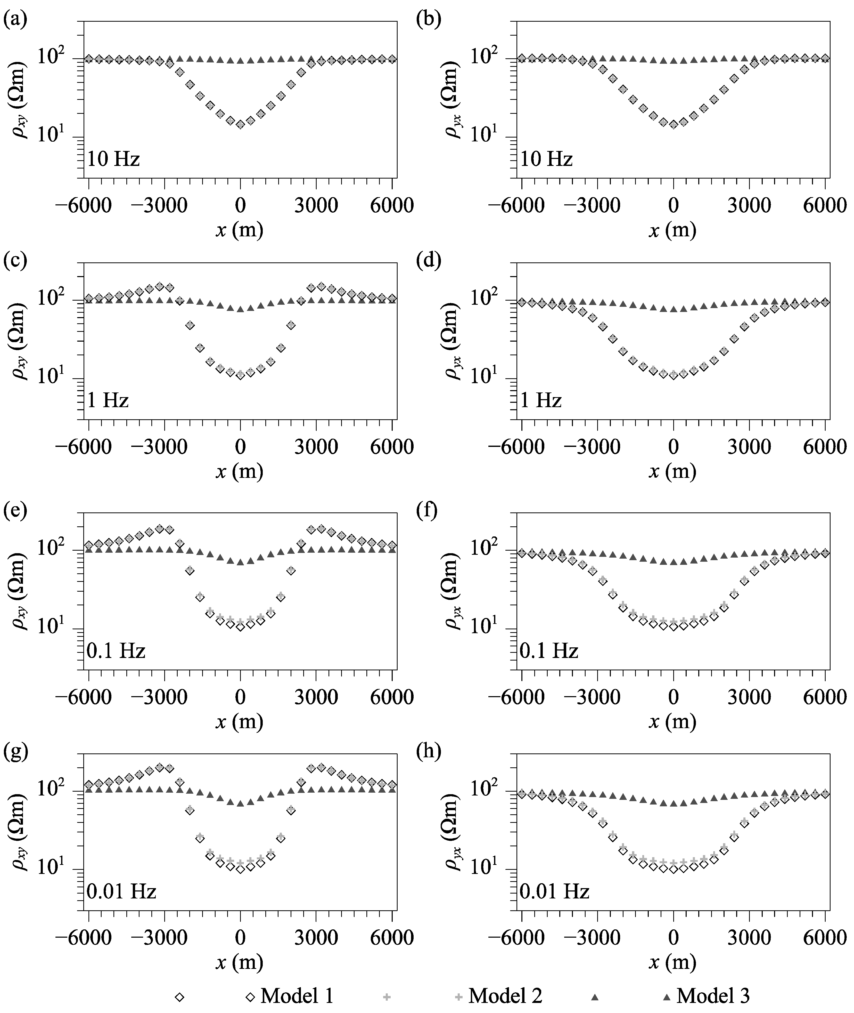
In order to separately study the characteristics of MT apparent resistivity induced by every part of the geothermal system, we set the reservoir resistivity to the half-space resistivity in Model 2 and set the resistivities of the smectite layer and illite-smectite mixed layer (clay cap) to that of the half-space resistivity in Model 3. Figure 6 shows the apparent resistivity curves for Models 1, 2, and 3, and the corresponding data for Model 1 are shown in

Table 4. The apparent resistivities calculated by the FE method for Model 1, as shown in Table 3. The apparent resistivity unit is Ωm. The y-coordinate is 0 m.

x (m)	ρxy				ρyx
	0.01 Hz	0.1 Hz	1 Hz	10 Hz	0.01 Hz	0.1 Hz	1 Hz	10 Hz
0	10.09	10.58	11.00	14.52	10.09	10.61	10.98	14.43
400	10.92	11.44	11.94	16.19	10.37	10.93	11.45	15.52
800	12.07	12.65	13.38	19.77	10.92	11.58	12.55	18.67
1200	14.98	15.56	16.35	25.21	11.72	12.50	14.17	23.28
1600	24.87	25.07	24.57	33.57	13.42	14.37	16.98	30.08
2000	56.70	54.80	47.84	46.77	17.39	18.55	22.30	40.44
2400	129.27	121.57	97.75	66.98	25.76	27.14	32.04	55.68
2800	195.05	182.13	143.62	85.74	38.74	40.28	45.93	72.81
3200	199.38	186.74	149.29	92.67	52.41	53.94	59.67	85.95
3600	180.44	169.86	138.78	94.35	63.73	65.07	70.34	93.53
4000	161.98	153.25	128.03	95.47	72.31	73.41	78.04	97.62
4400	147.89	140.54	119.83	96.43	78.65	79.48	83.45	99.62
4800	137.64	131.30	114.02	97.43	83.33	83.91	87.31	100.63
5200	130.13	124.54	109.86	98.13	86.84	87.21	90.08	100.97
5600	124.55	119.53	106.89	98.66	89.51	89.68	92.12	101.03
6000	120.41	115.82	104.78	98.90	91.58	91.58	93.65	100.87

. Both the ρ_xy and ρ_yx curves of Models 1 and 2 are in good agreement with each other for the frequencies of 10 and 1 Hz and then diverge from x = −1500 m to x = 1500 m as the frequency decreases. The ρ_xy and ρ_yx values for Model 3 are nearly the same as the half-space resistivity at all observation stations for the frequency of 10 Hz, and then gradually bends down from x = −1500 m to x = 1500 m as the frequency decreases. The minimum value of the ρ_xy curve is about 70 Ωm for Model 3 and is far larger than the corresponding ones for Models 2 and 3. It illustrates that the total EM responses for this hydrothermal system are dominated by the ones induced by the shallow, low-resistivity clay cap as the frequency decreases from 10 Hz to 0.01 Hz.

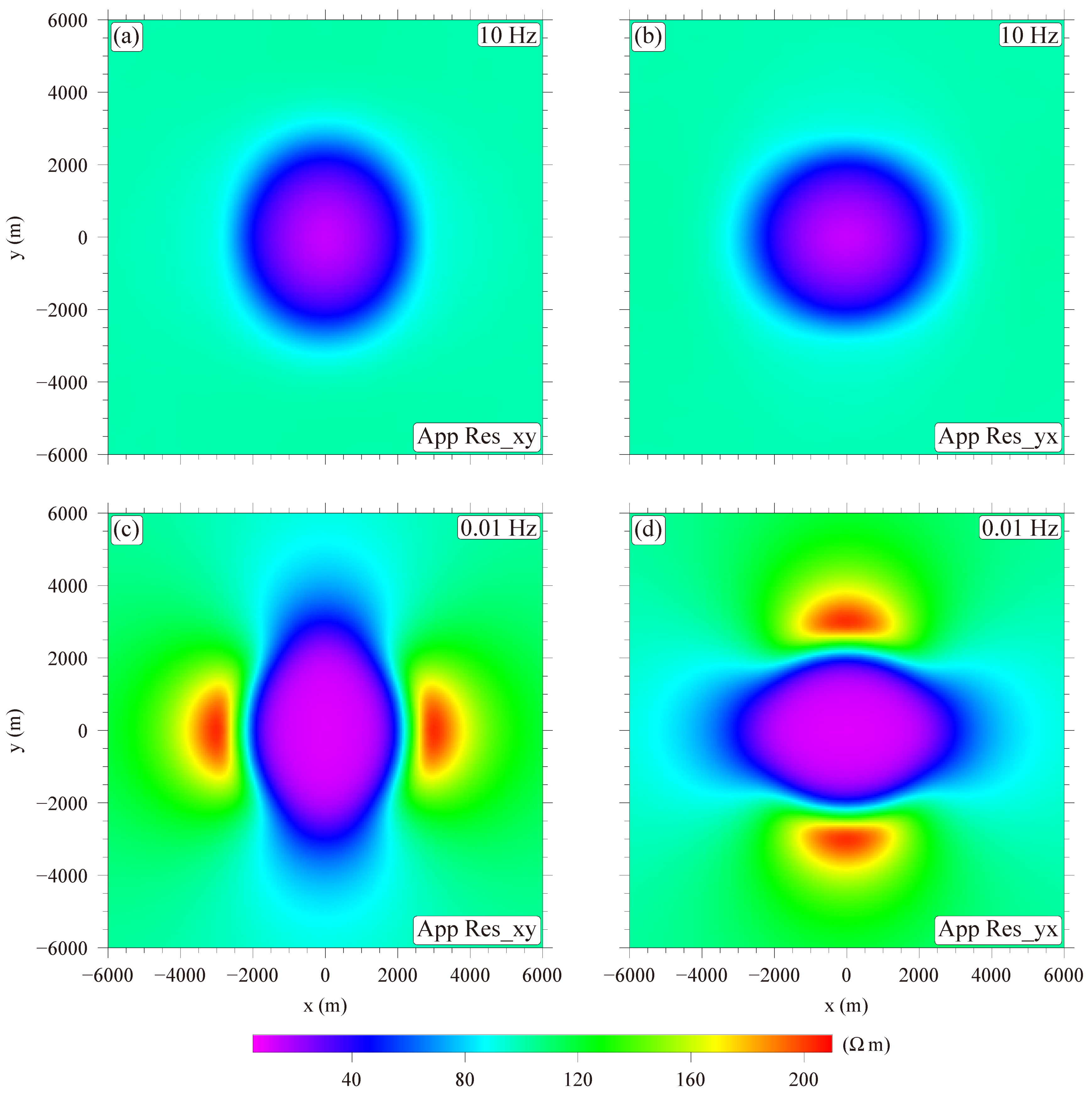
Figure 7 shows the contour map of ρ_xy and ρ_yx at 10 and 0.01 Hz for Model 1. The low apparent resistivities only occur in the central domain of these four contour maps (see Figure 7). As stated above, the EM responses associated with the shallow, low-resistivity clay cap are dominant in the total EM responses. Consequently, the low apparent resistivities associated with these domains are primarily caused by the clay cap, and secondarily by the reservoir. Figure 8 shows the vector maps of induction arrows for Model 1, and the corresponding data are shown in

Table 5. The real parts of the tipper transfer function calculated by the FE method for Model 1, as shown in Table 3. The y-coordinate is 0 m.

x (m)	Re (Tx)				Re (Ty)
	0.01 Hz	0.1 Hz	1 Hz	10 Hz	0.01 Hz	0.1 Hz	1 Hz	10 Hz
0	−8.04 × 10−4	1.40 × 10−5	−4.67 × 10−6	−5.52 × 10−4	5.91 × 10−4	−7.97 × 10−4	−1.29 × 10−4	−4.10 × 10−4
400	3.07 × 10−3	1.25 × 10−2	3.94 × 10−2	4.49 × 10−2	5.82 × 10−4	−7.80 × 10−4	−3.13 × 10−5	−1.18 × 10−4
800	6.28 × 10−3	2.28 × 10−2	7.21 × 10−2	7.43 × 10−2	5.74 × 10−4	−7.61 × 10−4	6.51 × 10−5	2.61 × 10−4
1200	9.08 × 10−3	3.18 × 10−2	1.01 × 10−1	9.83 × 10−2	5.49 × 10−4	−7.95 × 10−4	−2.39 × 10−5	2.79 × 10−4
1600	1.14 × 10−2	3.93 × 10−2	1.25 × 10−1	1.23 × 10−1	5.28 × 10−4	−8.16 × 10−4	−8.30 × 10−5	−5.03 × 10−6
2000	1.28 × 10−2	4.37 × 10−2	1.39 × 10−1	1.43 × 10−1	5.05 × 10−4	−8.47 × 10−4	−1.77 × 10−4	−5.79 × 10−5
2400	1.27 × 10−2	4.33 × 10−2	1.39 × 10−1	1.47 × 10−1	4.93 × 10−4	−8.47 × 10−4	−1.73 × 10−4	−8.38 × 10−5
2800	1.10 × 10−2	3.81 × 10−2	1.22 × 10−1	1.20 × 10−1	4.86 × 10−4	−8.42 × 10−4	−1.56 × 10−4	−6.29 × 10−5
3200	8.91 × 10−3	3.14 × 10−2	1.00 × 10−1	8.08 × 10−2	4.70 × 10−4	−8.67 × 10−4	−2.26 × 10−4	−2.56 × 10−4
3600	7.09 × 10−3	2.56 × 10−2	8.09 × 10−2	4.92 × 10−2	4.65 × 10−4	−8.54 × 10−4	−1.75 × 10−4	−1.12 × 10−4
4000	5.66 × 10−3	2.11 × 10−2	6.54 × 10−2	2.78 × 10−2	4.50 × 10−4	−8.71 × 10−4	−2.18 × 10−4	−2.15 × 10−4
4400	4.57 × 10−3	1.76 × 10−2	5.35 × 10−2	1.47 × 10−2	4.51 × 10−4	−8.35 × 10−4	−1.00 × 10−4	4.30 × 10−5
4800	3.70 × 10−3	1.49 × 10−2	4.41 × 10−2	6.43 × 10−3	4.46 × 10−4	−8.18 × 10−4	−3.54 × 10−5	1.66 × 10−4
5200	3.00 × 10−3	1.27 × 10−2	3.64 × 10−2	1.17 × 10−3	4.26 × 10−4	−8.46 × 10−4	−1.12 × 10−4	−9.42 × 10−5
5600	2.44 × 10−3	1.09 × 10−2	3.03 × 10−2	−1.91 × 10−3	4.08 × 10−4	−8.68 × 10−4	−1.73 × 10−4	−3.16 × 10−4
6000	1.99 × 10−3	9.47 × 10−3	2.54 × 10−2	−3.39 × 10−3	4.05 × 10−4	−8.41 × 10−4	−8.50 × 10−5	−1.20 × 10−4

. The direction of the induction arrows points outwards away from the central domain. The maximum values of their length at 10 and 1 Hz always concentrate in the inner and outer domains close to the circles marking the projections of the smectite-layer boundary on the surface. They mainly occur in the inner domain of the circles at 0.1 Hz. It illustrates that the induction arrows could reflect the hydrothermal system well.

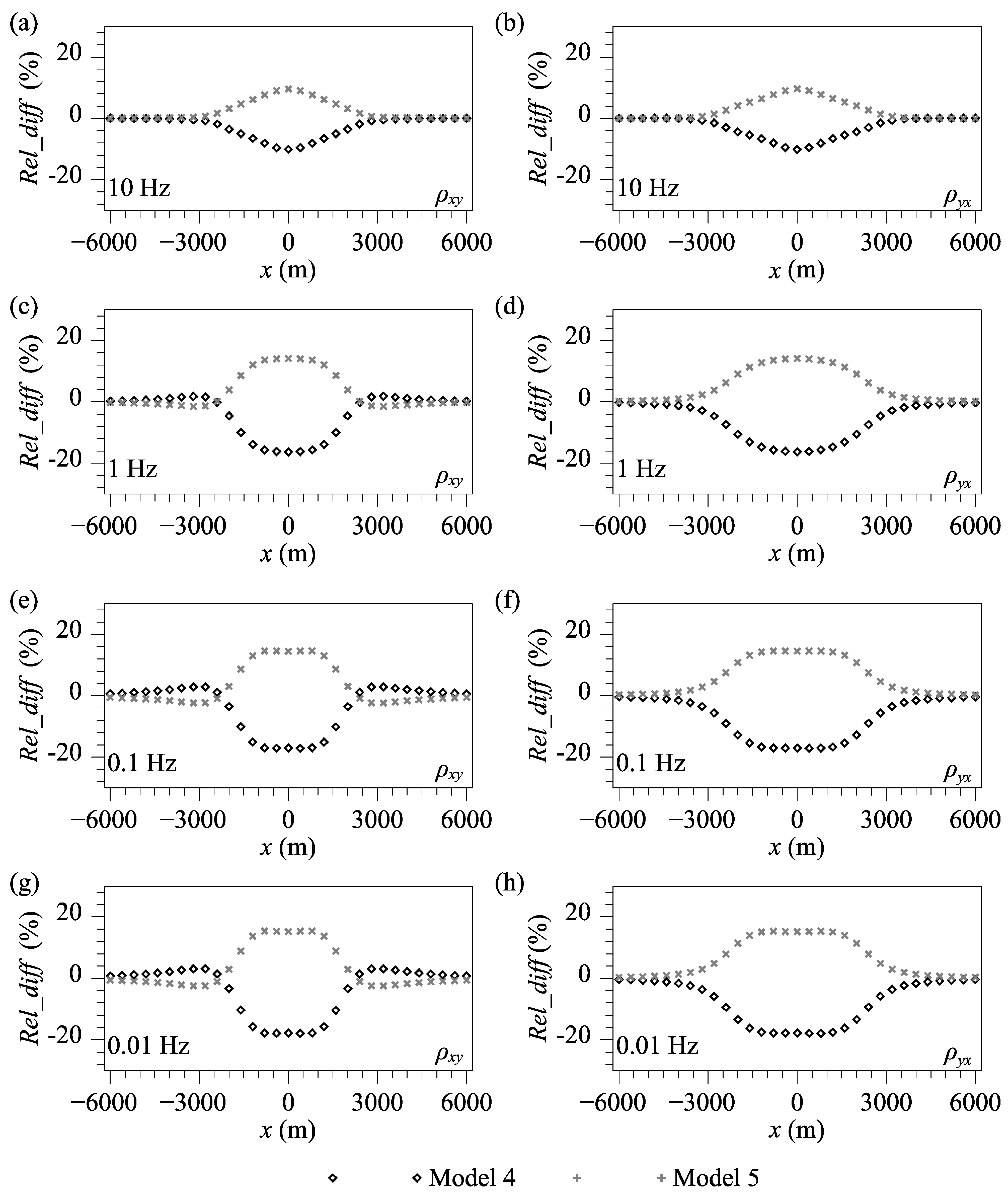
Then, we investigate the apparent resistivity characteristics as the resistivity of every part of the geothermal system is perturbed. The perturbing value is 20% of the resistivity of each part in Model 1. For example, the smectite-layer resistivity is 5 Ωm in Model 1, and it changes to 4 and 6 Ωm in Models 4 and 5, respectively. Figure 9, Figure 10 and Figure 11 show the apparent resistivity curves when the resistivities of the smectite layer, illite-smectite mixed layer, and reservoir being perturbed in turn. In these three figures, the relative difference between the apparent resistivities of Model 1 and a given perturbed model is calculated by the following formula:

$$rel\_diff\left(f\right)=100\times \left(app\_re{s}_{\mathrm{Perturbed} \mathrm{model}}\left(f\right)-app\_re{s}_{\mathrm{Model}1}\left(f\right)\right)/app\_re{s}_{\mathrm{Model}1}\left(f\right),$$

(15)

where $app\_re{s}_{\mathrm{Model}1}\left(f\right)$ and $app\_re{s}_{\mathrm{Perturbed} \mathrm{model}}\left(f\right)$ denote the apparent resistivities for Model 1 and the perturbed models at a given frequency f, respectively.

As shown in Figure 9, the absolute values of relative differences of ρ_xy and ρ_yx increase as the frequency decreases, and they are nearly identical for the frequencies of 0.1 and 0.01 Hz. This phenomenon also occurs in Figure 10 and Figure 11. In these two figures, the two relative difference curves are nearly coincident with each other for the frequency of 10 Hz, especially in Figure 11, and then gradually diverge. The maximum relative differences are about 16% in Figure 9g,h, and decrease to 8% in Figure 10g,h, and to 4% in Figure 11g,h. The above phenomena illustrate that the shallow conductive smectite layer and illite-smectite mixed layer have remarkable shielding effects on the deeper reservoir, and the changes in the reservoir resistivity have less important effects on apparent resistivities.

The effects of half-space resistivities on apparent resistivities are shown in Figure 12. The apparent-resistivity curves bend down when the x-coordinate ranges from −3000 m to 3000 m for all frequencies and models. For 10 and 1 Hz, the three apparent-resistivity curves nearly agree with each other between x = −1500 m and x = 1500 m and diverge elsewhere (see Figure 12a–d). For the two lower frequencies, the three apparent-resistivity curves diverge even for the x coordinate from −1500 m to 1500 m, and the minimum apparent resistivities decrease as the half-space resistivity increases (see Figure 12e–h). It confirms that a large resistivity contrast between an anomalous body (the hydrothermal system) and its surrounding host makes it easier to detect the anomalous body using the MT method.

3.3. HDR and Partial Melting System

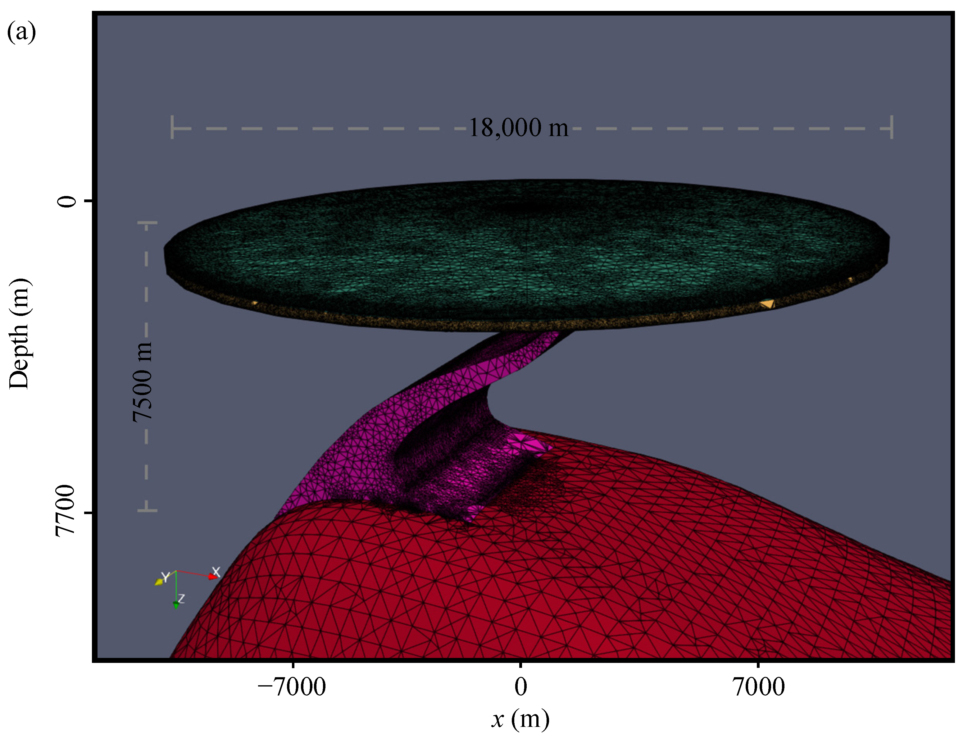
A series of models for an HDR and partial melting system are also investigated. Compared with models for a hydrothermal system, a more conductive heat source associated with a partial melting body is added to the synthesized models for an HDR and partial melting system. As shown in Figure 13, this geothermal system consists of clay cap, reservoir, path, and heat source. The reservoir and the heat source are connected by the heat-conducting path. For both the clay cap and reservoir the thickness was set to 240 m, and the lengths both in the x- and y-directions were set to 18,000 m. The numbers for both observation lines and station are still 41, but the interval is 1000 m. The computational domain is divided into 19,540,394 tetrahedra.

The resistivity values for each part of Model 12 are listed in

Table 6. The assigned resistivity values for the HDR and partial melting system, as shown in Figure 13. The resistivity unit is Ωm.

Model	Air	Half-Space	Clay Cap	Reservoir	Path/Heat Source
Model 12	1012	200	5	10	1
Model 13	1012	200	5	10	200
Model 14	1012	200	200	200	1

. Here we also set the resistivities of the path and the heat source to 200 Ωm in Model 13 and set the resistivities of the clay cap and reservoir to 200 Ωm in Model 14 in order to study the apparent-resistivity characteristics caused by every part of the geothermal system separately. Figure 14 shows the apparent resistivity curves for Models 12, 13, and 14, and the corresponding data for Model 12 are shown in

Table 7. The apparent resistivities calculated by the FE method for Model 12, as shown in Table 6. The apparent resistivity unit is Ωm. The y-coordinate is 0 m.

x (m)	ρxy			ρyx
	0.001 Hz	0.1 Hz	10 Hz	0.001 Hz	0.1 Hz	10 Hz
0	15.93	15.35	12.47	10.47	17.97	12.63
100	17.03	15.73	15.82	8.98	17.14	15.87
2000	14.69	17.99	19.93	6.74	15.37	21.07
3000	7.34	33.89	23.44	7.29	16.69	25.09
4000	6.86	33.87	27.75	9.66	20.02	27.76
5000	7.13	31.69	33.07	11.42	22.75	32.67
6000	7.02	28.52	38.82	12.41	24.59	38.04
7000	6.89	25.92	44.83	12.84	25.81	42.91
8000	9.85	32.73	54.20	13.14	27.14	48.47
9000	66.57	181.30	102.76	15.67	33.12	73.91
10,000	170.27	435.92	188.26	26.28	54.03	144.02
11,000	136.90	331.86	191.30	37.99	75.41	185.30
12,000	115.04	259.26	192.98	47.39	91.47	199.74
13,000	106.17	220.47	196.06	55.01	103.56	202.91
14,000	104.01	198.28	197.21	61.46	113.13	203.17
15,000	105.83	185.22	198.30	67.15	120.95	202.10
16,000	110.25	177.47	199.47	72.37	127.67	201.80
17,000	116.48	172.77	200.39	77.31	133.53	201.34
18,000	124.12	170.06	200.30	82.08	138.78	201.20
19,000	132.72	168.84	200.79	86.70	143.48	200.62
20,000	142.06	168.77	202.44	91.24	147.88	200.92

. The ρ_xy and ρ_yx curves for Model 13 are always symmetrical at all frequencies due to the symmetrical shapes of the clay cap and reservoir. The ρ_xy and ρ_yx values for Model 14 seem to be the same as the half-space resistivity at 10 Hz, except for ρ_yx at several observation stations, and then decrease to various levels for all observation stations at 0.1 and 0.001 Hz because of the irregular shapes of the path and heat source. Hence both the ρ_xy and ρ_yx curves of Model 12 match well with the ones of Model 13 at 10 Hz, and then present a complex shape at 0.1 and 0.001 Hz due to the effects of the path and heat source. It indicates that the total EM responses for the HDR and partial melting system are dominated by the responses caused by the shallow low-resistivity clay cap and reservoir at 10 Hz, and are dramatically affected by the path and heat source at lower frequencies, especially at 0.001 Hz.

Figure 15 shows the contour maps of ρ_xy and ρ_yx at 10, 0.1, and 0.001 Hz for Model 12. The low apparent resistivities mainly occur in the central part of these six contour maps (see Figure 15). Unlike the symmetrical low-apparent-resistivity domains at 10 Hz, the ones at 0.1 and 0.001 Hz are not symmetrical about the x-coordinate (see Figure 15c–f). It demonstrates that the regions with low apparent resistivity are mainly associated with the symmetrically shaped clay cap and reservoir at 10 Hz, as well as associated with all parts of this geothermal system at 0.1 and 0.001 Hz. These characteristics also appear in the vector maps of induction arrows for Model 12 (see Figure 16 and Figure 17). As shown in Figure 16, the vector maps of Model 13 are symmetrical about both the x- and y-axes, because of the symmetry of this model. 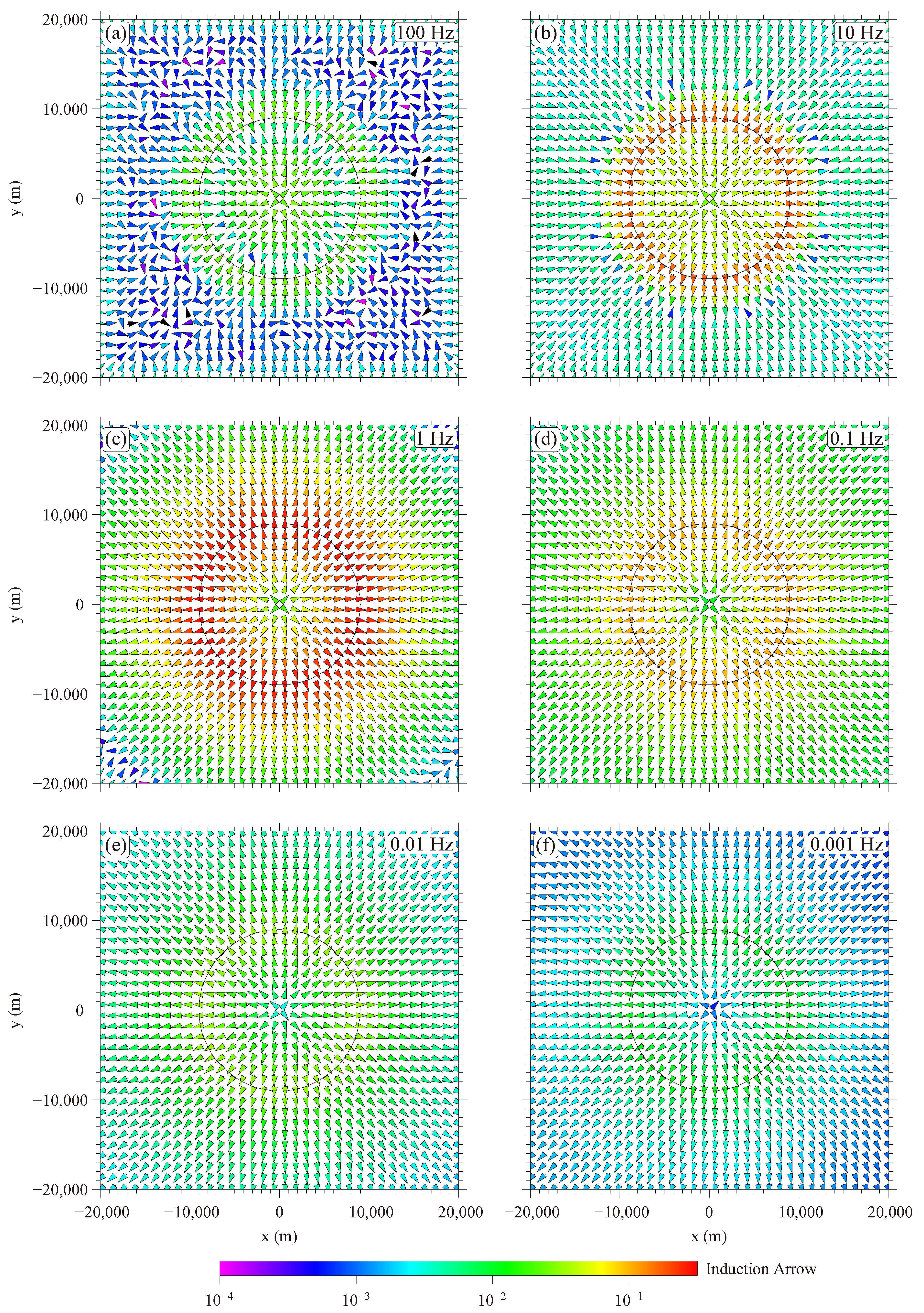Figure 17 is the vector map for Model 12, which has an un-symmetrical electrical structure. Compared with these two figures, the vector maps for the frequencies of 0.1, 0.01, and 0.001 Hz are different in the symmetrical pattern and the magnitudes of the vector arrows. It can be inferred that the path and heat source can cause significant EM responses for the HDR and partial melting system at these three lower fre-quencies. The corresponding data of Figure 17 are shown in

Table 8. The real parts of the tipper transfer function calculated by the FE method for Model 12, as shown in Table 6. The y-coordinate is 0 m.

x (m)	Re (Tx)			Re (Ty)
	0.001 Hz	0.1 Hz	10 Hz	0.001 Hz	0.1 Hz	10 Hz
0	−4.39 × 10−3	−1.12 × 10−2	1.96 × 10−3	−3.04 × 10−4	−6.93 × 10−4	−1.48 × 10−4
100	−2.12 × 10−3	9.33 × 10−3	4.71 × 10−2	−2.89 × 10−4	−6.22 × 10−4	−5.33 × 10−5
2000	3.56 × 10−4	3.37 × 10−2	4.76 × 10−2	−2.81 × 10−4	−6.21 × 10−4	7.69 × 10−5
3000	3.35 × 10−3	6.59 × 10−2	3.06 × 10−2	−2.82 × 10−4	−6.81 × 10−4	−1.44 × 10−4
4000	5.19 × 10−3	8.02 × 10−2	4.04 × 10−2	−2.75 × 10−4	−6.97 × 10−4	−3.83 × 10−4
5000	6.59 × 10−3	8.70 × 10−2	4.34 × 10−2	−2.61 × 10−4	−6.48 × 10−4	−1.43 × 10−4
6000	8.02 × 10−3	9.38 × 10−2	4.28 × 10−2	−2.59 × 10−4	−7.13 × 10−4	−3.51 × 10−4
7000	9.59 × 10−3	1.02 × 10−1	4.30 × 10−2	−2.50 × 10−4	−6.86 × 10−4	−2.04 × 10−4
8000	1.14 × 10−2	1.13 × 10−1	7.00 × 10−2	−2.34 × 10−4	−6.37 × 10−4	−1.86 × 10−4
9000	1.30 × 10−2	1.23 × 10−1	1.63 × 10−1	−2.24 × 10−4	−6.19 × 10−4	1.59 × 10−5
10,000	1.29 × 10−2	1.15 × 10−1	1.42 × 10−1	−2.19 × 10−4	−6.22 × 10−4	−1.53 × 10−5
11,000	1.25 × 10−2	1.03 × 10−1	6.04 × 10−2	−2.09 × 10−4	−6.14 × 10−4	−5.23 × 10−5
12,000	1.23 × 10−2	9.53 × 10−2	1.92 × 10−2	−1.96 × 10−4	−6.01 × 10−4	−2.89 × 10−4
13,000	1.24 × 10−2	8.95 × 10−2	2.12 × 10−3	−1.87 × 10−4	−5.91 × 10−4	−3.10 × 10−4
14,000	1.25 × 10−2	8.49 × 10−2	−4.13 × 10−3	−1.75 × 10−4	−5.64 × 10−4	−2.25 × 10−4
15,000	1.27 × 10−2	8.11 × 10−2	−5.50 × 10−3	−1.65 × 10−4	−5.44 × 10−4	−1.61 × 10−4
16,000	1.28 × 10−2	7.77 × 10−2	−5.47 × 10−3	−1.52 × 10−4	−5.15 × 10−4	−2.23 × 10−4
17,000	1.29 × 10−2	7.46 × 10−2	−4.83 × 10−3	−1.46 × 10−4	−5.16 × 10−4	−1.40 × 10−4
18,000	1.30 × 10−2	7.18 × 10−2	−4.58 × 10−3	−1.34 × 10−4	−4.89 × 10−4	−1.42 × 10−4
19,000	1.31 × 10−2	6.91 × 10−2	−4.38 × 10−3	−1.23 × 10−4	−4.77 × 10−4	−3.71 × 10−4
20,000	1.31 × 10−2	6.65 × 10−2	−3.87 × 10−3	−1.14 × 10−4	−4.75 × 10−4	−6.84 × 10−4

.

4. Conclusions

A 3D vector FE forward modeling approach is developed to investigate the MT response characteristics of two typical magmatic geothermal systems, namely a hydrothermal system and an HDR and partial melting system. The results show that the apparent resistivities at broadband frequencies are mainly affected by the shallow, low-resistivity clay cap due to its strong shielding effects, and the induction arrows effectively reflect the boundary of the conductive cap for both geothermal systems. The conductive heat conducting path and heat source (1 S/m) considered in the models of HDR and partial melting system could induce dramatical changes to the apparent resistivities and induction arrows at lower frequencies. As stated above, the induction arrows can be used to delineate the lateral boundaries of the low-resistivity clay cap, heat conducting path, and heat source. If the induction arrow data are available, they should be complementary to the apparent resistivities for better lateral resolution when processing and inverting MT data.

References

1. Muñoz, G. Exploring for geothermal resources with electromagnetic methods. Surv. Geophys. 2014, 35, 101–122. [Google Scholar] [CrossRef]
2. Spichak, V.; Manzella, A. Electromagnetic sounding of geothermal zones. J. Appl. Geophys. 2009, 68, 459–478. [Google Scholar] [CrossRef]
3. Gumming, W. A conceptual model approach to the geophysical exploration of permeable geothermal reservoirs that considers context and uncertainty. SEG Tech. Program Expand. Abstr. 2009, 4326–4330. [Google Scholar]
4. Gao, J.; Zhang, H.; Zhang, S.; Chen, X.; Cheng, Z.; Jia, X.; Li, S.; Fu, L.; Gao, L.; Xin, H. Three-dimensional magnetotelluric imaging of the geothermal system beneath the Gonghe Basin, Northeast Tibetan Plateau. Geothermics 2018, 76, 15–25. [Google Scholar] [CrossRef]
5. Zhou, W.; Hu, X.; Guo, H.; Liu, S.; Liu, S.; Yang, B. Three-dimensional magnetotelluric inversion reveals the typical geothermal structure of Yanggao geothermal field in Datong Basin, northern China. Geothermics 2022, 105, 102505. [Google Scholar] [CrossRef]
6. Peacock, J.R.; Thiel, S.; Reid, P.; Heinson, G. Magnetotelluric monitoring of a fluid injection: Example from an enhanced geothermal system. Geophys. Res. Lett. 2012, 39, L18403. [Google Scholar] [CrossRef] [Green Version]
7. Peacock, J.R.; Mangan, M.T.; McPhee, D.; Wannamaker, P.E. Three-dimensional electrical resistivity model of the hydrothermal system in Long Valley Caldera, California, from magnetotellurics. Geophys. Res. Lett. 2016, 43, 7953–7962. [Google Scholar] [CrossRef]
8. Newman, G.A.; Gasperikova, E.; Hoversten, G.M.; Wannamaker, P.E. Three-dimensional magnetotelluric characterization of the Coso geothermal field. Geothermics 2008, 37, 369–399. [Google Scholar] [CrossRef]
9. Bibby, H.M.; Risk, G.F.; Caldwell, T.G.; Heise, W. Investigations of deep resistivity structures at the Wairakei geothermal field. Geothermics 2009, 38, 98–107. [Google Scholar] [CrossRef]
10. Tian, H.-J.; Zhang, G.-D.; Liu, G.-D.; You, W.-B.; Zhang, Y.-W. The application effect of the wide field electromagnetic method in geothermal exploration of Tailong area, northern Guizhou Province. Geophys. Geochem. Explor. 2020, 44, 1093–1097. [Google Scholar]
11. Árnason, K.; Eysteinsson, H.; Hersir, G.P. Joint 1D inversion of TEM and MT data and 3D inversion of MT data in the Hengill area, SW Iceland. Geothermics 2010, 39, 13–34. [Google Scholar] [CrossRef]
12. Gamble, T.D.; Goubau, W.M.; Clarke, J. Magnetotellurics with a remote magnetic reference. Geophysics 1979, 44, 53–68. [Google Scholar] [CrossRef]
13. Egbert, G.D. Robust multiple-station magnetotelluric data processing. Geophys. J. Int. 1997, 130, 475–496. [Google Scholar] [CrossRef] [Green Version]
14. Ryan, G.A.; Peacock, J.R.; Shalev, E.; Rugis, J. Montserrat geothermal system: A 3D conceptual model. Geophys. Res. Lett. 2013, 40, 2038–2043. [Google Scholar] [CrossRef]
15. Samrock, F.; Kuvshinov, A.; Bakker, J.; Jackson, A.; Fisseha, S. 3-D analysis and interpretation of magnetotelluric data from the Aluto-Langano geothermal field, Ethiopia. Geophys. J. Int. 2015, 202, 1923–1948. [Google Scholar] [CrossRef] [Green Version]
16. Peacock, J.R.; Thiel, S.; Heinson, G.S.; Reid, P. Time-lapse magnetotelluric monitoring of an enhanced geothermal system. Geophysics 2013, 78, B121–B130. [Google Scholar] [CrossRef]
17. Liu, C.; Ren, Z.; Tang, J.; Yan, Y. Three-dimensional magnetotellurics modeling using edge-based finite-element unstructured meshes. Appl. Geophys. 2008, 5, 170–180. [Google Scholar] [CrossRef]
18. Ren, Z.; Kalscheuer, T.; Greenhalgh, S.; Maurer, H. A goal-oriented adaptive finite-element approach for plane wave 3-D electromagnetic modelling. Geophys. J. Int. 2013, 194, 700–718. [Google Scholar] [CrossRef] [Green Version]
19. Jin, J.-M. The Finite Element Method in Electromagnetics; John Wiley & Sons: New York, NY, USA, 2014. [Google Scholar]
20. Farquharson, C.G.; Miensopust, M.P. Three-dimensional finite-element modelling of magnetotelluric data with a divergence correction. J. Appl. Geophys. 2011, 75, 699–710. [Google Scholar] [CrossRef]
21. Weaver, J.T. Mathematical Methods for Geo-Electromagnetic Induction; Research Studies Press: Taunton, UK, 1994. [Google Scholar]
22. Amestoy, P.R.; Guermouche, A.; L’Excellent, J.-Y.; Pralet, S. Hybrid scheduling for the parallel solution of linear systems. Parallel Comput. 2006, 32, 136–156. [Google Scholar] [CrossRef] [Green Version]
23. Long, J.; Farquharson, C.G. On the forward modelling of three-dimensional magnetotelluric data using a radial-basis-function-based mesh-free method. Geophys. J. Int. 2019, 219, 394–416. [Google Scholar] [CrossRef]
24. Tang, J.; Jin, G.; Zhao, G.; Li, W.; Xuan, F.; Bai, D.; Zhan, D. Induction arrow and its application in Tianchi volcano, Changbai mountains. Geol. Rev. 1999, 45, 294–303. [Google Scholar]
25. Wiese, H. Geomagnetische Tiefentellurik Teil II: Die Streichrichtung der Untergrundstrukturen des elektrischen Widerstandes, erschlossen aus geomagnetischen Variationen. Geofis. Pura Appl. 1962, 52, 83–103. [Google Scholar] [CrossRef]
26. Zhdanov, M.; Varentsov, I.; Weaver, J.; Golubev, N.; Krylov, V. Methods for modelling electromagnetic fields results from COMMEMI the international project on the comparison of modelling methods for electromagnetic induction. J. Appl. Geophys. 1997, 37, 133–271. [Google Scholar] [CrossRef]
27. Si, H. TetGen: A Delaunay-based quality tetrahedral mesh generator. ACM Trans. Math. Softw. 2015, 41, 1–36. [Google Scholar] [CrossRef]
28. Li, J.; Hu, X.; Zhang, K.; Yuan, W.; Gang, T. Synthesizing TEM data by a 3D FETD approach: A case study of delineating a resistive basaltic body located in the Narenbaolige coalfield, China. SEG Tech. Program Expand. Abstr. 2020, 621–625. [Google Scholar] [CrossRef]
Figure 1. A flowchart of the FE method used in this study for calculating MT responses.
Energies 15 09282 g001
Figure 2. The tetrahedral grids of the COMMEMI 3D-1A model [23]. (a) The bird’s-eye view of the conductive block. (b) The plane view at z = 0 m, with the white points denoting the observation points. (c) The section view at y = 0 m. (d) The section view at x = 0 m.
Energies 15 09282 g002
Figure 3. The apparent resistivities of 0.1 Hz for the COMMEMI 3D-1A model. (a,b) are for ρxy and ρyx for the x-directed survey line, respectively. (c,d) are for ρxy and ρyx for the y-directed survey line, respectively.
Energies 15 09282 g003
Figure 4. The induction arrow for the COMMEMI 3D-1A model. (ad) are for the frequencies of 100, 10, 1, and 0.1 Hz, respectively. The black rectangles indicate the projection of the conductive blocks on the x-y plane.
Energies 15 09282 g004
Figure 5. The tetrahedral grids of a typical hydrothermal system. (a) The bird’s-eye view of the conductive block. (b) The section view at y = 0 m.
Energies 15 09282 g005
Figure 6. The curves of apparent resistivity for the models representing the hydrothermal system, as shown in Figure 5. The resistivity information of Models 1, 2, and 3 is shown in Table 3. (a,b) are for 10 Hz, (c,d) are for 1 Hz; (e,f) are for 0.1 Hz, (g,h) are for 0.01 Hz.
Energies 15 09282 g006
Figure 7. The contour maps of the apparent resistivities for Model 1 of the typical hydrothermal system, as shown in Figure 5. (a,b) are for 10 Hz, (c,d) are for 0.01 Hz.
Energies 15 09282 g007
Figure 8. The vector maps of induction arrows for Model 1 of the typical hydrothermal system, as shown in Figure 5. (ad) are for the frequencies of 10, 1, 0.1, and 0.01 Hz, respectively. The black circles indicate the projection of the clay cap on the x-y plane.
Energies 15 09282 g008
Figure 9. The relative differences between the apparent resistivities of Model 1, and Models 4 and 5. Models 4 and 5 are obtained by perturbing the smectite-layer resistivity of Model 1 by 20% of its value. (a,b) are for 10 Hz, (c,d) are for 1 Hz; (e,f) are for 0.1 Hz, and (g,h) are a for 0.01 Hz.
Energies 15 09282 g009
Figure 10. The relative differences between the apparent resistivities of Model 1, and Models 6 and 7. Models 6 and 7 are obtained by perturbing the smectite-illite-mixed-layer resistivity of Model 1 by 20% of its value. (a,b) are for 10 Hz, (c,d) are for 1 Hz; (e,f) are for 0.1 Hz, and (g,h) are for 0.01 Hz.
Energies 15 09282 g010
Figure 11. The relative differences between the apparent resistivities of Model 1, and Models 8 and 9. Models 8 and 9 are obtained by perturbing the reservoir resistivity of Model 1 by 20% of its value. (a,b) are for 10 Hz, (c,d) are for 1 Hz; (e,f) are for 0.1 Hz, and (g,h) are for 0.01 Hz.
Energies 15 09282 g011
Figure 12. The curves of apparent resistivity for the models representing the hydrothermal system, as shown in Figure 5. The resistivity information of Models 1, 10, and 11 are shown in Table 3. (a,b) is for 10 Hz, (c,d) are for 1 Hz; (e,f) are for 0.1 Hz, (g,h) are for 0.01 Hz.
Energies 15 09282 g012
Figure 13. The tetrahedral grids of an HDR and partial melting system. (a) The bird’s-eye view of the conductive block. (b) The section view of y = 0 m.
Energies 15 09282 g013aEnergies 15 09282 g013b
Figure 14. The curves of apparent resistivity for the models representing the HDR and partial melting system, as shown in Figure 13. The resistivity information of Models 12, 13, and 14 are shown in Table 6. (a,b) is for 10 Hz, (c,d) is for 0.1 Hz; (e,f) is for 0.001 Hz.
Energies 15 09282 g014
Figure 15. The contour maps of the apparent resistivities for the HDR and partial melting system, as shown in Figure 13. (a,b) are for 10 Hz, (c,d) are for 0.1 Hz, and (e,f) are for 0.001 Hz.
Energies 15 09282 g015
Figure 16. The vector maps of the induction arrows of Model 13 for the HDR and partial melting system, as shown in Figure 13. (af) are for the frequencies of 100, 10, 1, 0.1, 0.01, and 0.001 Hz, respectively. The black circles indicate the projection of the clay cap on the x-y plane.
Energies 15 09282 g016
Figure 17. The vector maps of the induction arrows of Model 12 for the HDR and partial melting system, as shown in Figure 13. (af) are for the frequencies of 100, 10, 1, 0.1, 0.01, and 0.001 Hz, respectively. The black circles indicate the projection of the clay cap on the x-y plane.
Energies 15 09282 g017