Article

Wind Power Forecasting Using Optimized Dendritic Neural Model Based on Seagull Optimization Algorithm and Aquila Optimizer

by
Mohammed A. A. Al-qaness
1,*,
Ahmed A. Ewees
2,3,
Mohamed Abd Elaziz
4,5,6,7 and
Ahmed H. Samak
2,8
1
College of Physics and Electronic Information Engineering, Zhejiang Normal University, Jinhua 321004, China
2
College of Computing and Information Technology, University of Bisha, Bisha 61922, Saudi Arabia
3
Department of Computer, Damietta University, Damietta 34517, Egypt
4
Department of Mathematics, Faculty of Science, Zagazig University, Zagazig 44519, Egypt
5
Faculty of Computer Science & Engineering, Galala University, Suze 435611, Egypt
6
Artificial Intelligence Research Center (AIRC), Ajman University, Ajman 346, United Arab Emirates
7
Department of Electrical and Computer Engineering, Lebanese American University, Byblos 13518, Lebanon
8
Faculty of Science, Menofia University, Shibeen El-Kom 32511, Egypt
*
Author to whom correspondence should be addressed.
Energies 2022, 15(24), 9261; https://doi.org/10.3390/en15249261
Submission received: 11 November 2022 / Revised: 29 November 2022 / Accepted: 5 December 2022 / Published: 7 December 2022
(This article belongs to the Special Issue Forecasting Techniques for Power Systems with Machine Learning)

Abstract

:
It is necessary to study different aspects of renewable energy generation, including wind energy. Wind power is one of the most important green and renewable energy resources. The estimation of wind energy generation is a critical task that has received wide attention in recent years. Different machine learning models have been developed for this task. In this paper, we present an efficient forecasting model using naturally inspired optimization algorithms. We present an optimized dendritic neural regression (DNR) model for wind energy prediction. A new variant of the seagull optimization algorithm (SOA) is developed using the search operators of the Aquila optimizer (AO). The main idea is to apply the operators of the AO as a local search in the traditional SOA, which boosts the SOA’s search capability. The new method, called SOAAO, is employed to train and optimize the DNR parameters. We used four wind speed datasets to assess the performance of the presented time-series prediction model, called DNR-SOAAO, using different performance indicators. We also assessed the quality of the SOAAO with extensive comparisons to the original versions of the SOA and AO, as well as several other optimization methods. The developed model achieved excellent results in the evaluation. For example, the SOAAO achieved high R 2 results of 0.95, 0.96, 0.95, and 0.91 on the four datasets.

1. Introduction

There has been significant attention on green energy because of the issues of ecological environmental balance and the wastefulness of traditional energy. Therefore, world interest has been directed towards green and renewable energy such as wind power [1]. However, it is difficult to control wind turbines and their operating systems. There are great challenges facing wind farm generation [2,3]. Therefore, excellent forecasting models are required to apply these systems properly. These models include production and repair scheduling, security evaluation, and energy transactions [4]. As a result, there are many prediction approaches that forecast wind energy. These approaches include statistical approaches, physical approaches, artificial intelligence (AI) approaches, and hybrid approaches [5,6]. These approaches show highly efficient long-term prediction, especially physical forecasting approaches, such as weather prediction [7].
In fact, the atmospheric information required adds significant computation complexity to solving wind speed prediction problems [8]. Statistical approaches, which include, for example, auto-regression and the autoregressive integrated moving average, are not complicated and can have accuracy better than other short-term prediction methods [9,10]. Unfortunately, these methods cannot effectively predict the non-linear and non-stationary wind speed because of the nature of statistical methods [11,12,13,14].
Intelligence models are effective and are extensively used to accurately forecast wind energy. This can be seen clearly in least squares support vector machines (SVMs) and neural networks. The most popular non-linear systems are artificial neural networks (ANNs), which are able to extract unclear functional relationships from historical time series. ANNs can develop themselves to be robust tools to predict wind energy [15,16]. Li and Shi [17], for example, produced a complete comparison on the study of the prediction performance of different ANNs. This study was based on data taken every hour in the state of North Dakota (USA).
Ping and Zhenkun [18] introduced a new approach based on ANNs. Their model is a hybrid model called NCFM that can measure short-term wind speed. It features the first patent data pretreatment technique adopted to decompose initial wind speed data. Then, the model analyzes the data to reconstitute it. It is an effective model because it can perform predictions against the varying wind speed series. Hao et al. [19] presented a hybrid wind power prediction approach where they extract the characteristics of every subseries using a two-layer decomposition method. Both layers are based on decomposition; the first layer, called EMD, is used to decompose wind power speed time series. The second layer, called VMD, is applied to decompose the IMF1 created by the EMD layer with more detailed coefficients.
Pei et al. [20] also tried to develop an accurate hybrid model with several stages. First, they applied an improved complete model for decomposition with adaptive noise techniques. This technique is based on eliminating noise and easily obtaining original data. Then, they built and used a wavelet neural network with the optimization method to achieve high accuracy. Finally, four examples and eighteen comparison models were used to test the abilities of the models. Jiaojiao et al. [21] presented a new hybrid model for wind speed forecasting. Firstly, they use complete ensemble empirical decomposition to separate wind power time series and obtain multiple components. These components were extracted using an optimized SVM. Then, they introduced a wind speed forecasting model using a modified CNN. Finally, they compared the proposed method with other models using real data on wind power to show how the validity of their method. Huang and Wang [22] proposed a wind energy forecasting model using an optimized LSTM model based on an improved version of the particle swarm optimization algorithm. They found that the improved PSO had a significant impact on the performance of the LSTM. In [23], the authors developed a multistep Informer model for adding meteorological parameters to wind energy generation prediction. This model was compared to the original Informer network and recorded better results. In [24], the authors applied the gradient boosting machine model combined with nonparametric regression and the mutual information coefficient to build a wind power estimation model. This combined method was successfully employed for short-term forecasting problems. In [25], an optimization method called the Optuna optimization framework was applied to optimize LSTM hyperparameters to improve the forecasting ability of an LSTM. They compared the optimized LSTM model to ARIMA and the original LSTM, concluding that the optimized LSTM model recorded the best wind power prediction results. Dendritic neural regression (DNR) has also been employed for wind power estimation and prediction. For example, in [26], an optimized DNR was applied for wind forecasting. The authors used states of matter search (SMS) to optimize DNR. Thus, the application of the SMS method improved DNR forecasting capability. In [27], the authors evaluated the dendritic neuron model for wind speed forecasting. They used the L-SHADE optimization algorithm to train the dendritic model to boost its prediction performance. In [28], an optimization method called the artificial immune system was used to train a dendritic neural model. This optimized model was applied for wind speed forecasting and showed competitive performance compared to other models.

Motivation and Contributions

Artificial neural networks are utilized in different research and engineering domains, including time series forecasting and prediction. Spiking neural networks (SNNs) are the third generation of ANNs, but they suffer from several critical issues, such as lacking effective training methods, meaning that they face problems in real-world applications. Furthermore, the encoding mechanisms of SNRs are not understood. Additionally, they have high computation costs [29,30]. To address these challenges, a new model, called the dynamic dendritic structure, was proposed by [31,32]. It was the initial structure of the current dendritic neuron model. Its main structure is comprised of a cell body and several layers called the synaptic, dendritic, and membrane layers. In recent years, the dendritic neuron model has been adopted in various applications, especially in time series forecasting and prediction such as economic tourism prediction [33], stock price prediction [34], PM2.5 concentration prediction [35], and COVID-19 pandemic prediction [36].
However, the dendritic neuron model faces certain limitations in the parameter configuration process. To this end, in recent years, advances in metaheuristic (MH) optimization algorithms have been adopted to boost the performance of the dendritic neuron model by training and optimizing its parameters, as in the genetic algorithm [34], the cuckoo search (CS) algorithm [37], and particle swarm optimization [38].
Following this concept, in this study, we present an efficient MH optimization method to train and optimize the parameters of a dendritic neuron model based on two algorithms: the seagull optimization algorithm (SOA) and the Aquila optimizer (AO). Hybrid metaheuristic optimization approaches aim to overcome the limitations of stand-alone MH optimization algorithms. To this end, we leveraged the advantages of the combination of SOA and AO to avoid their individual shortcomings. The SOA was proposed by [39] as a new bio-inspired MH optimization technique. It was inspired based on the natural behavior (i.e., attacking and migration) of a seagull. It has been utilized in different applications due to its good performance, such as in COVID-19 prediction [40], parameter estimation of photovoltaic models [41], dynamic optimization problems [42], routing problems in wireless sensor networks (WSN) [43], engineering design problems [44], and different optimization problems [45,46,47,48,49]. The AO is also a new natural-inspired MH optimization method. It was inspired by the natural behaviors of Aquila in attacking and hunting [50]. It received significant attention in recent years in solving different problems such as time series forecasting [51], medical image processing, feature selection for human activity recognition [52], feature selection for intrusion detection systems [53], wind power forecasting [54], and other optimization and engineering problems [55,56].
In this study, a new combined method, called the SOAAO optimization technique, is developed by combining the proprieties of the traditional SOA and AO. The main idea is to use the search parameters of the AO as a local search in the traditional SOA. Then, the developed SOAAO is utilized to train and optimize the parameters of the dendritic neuron model. The optimized dendritic neuron model is applied to forecast wind power using real-world datasets collected over three years (2017–2020) from four turbines in France. Additionally, we compared the performance of the new optimized model to the traditional dendritic neuron model, as well as to several optimized dendritic neuron schemes using well-known optimization methods, including the conventional versions of the AO and SOA algorithms.
The main contributions of this study are summarized as follows:
  • A new time series forecasting model for wind power is presented using an optimized dendritic neuron model;
  • A new optimization method is proposed based on the combination of SOA and AO algorithms. The combined method, called SOAAO, is utilized for training and optimizing the parameters of the dendritic neuron model to boost its forecasting ability;
  • Several MH optimization algorithms for training dendritic neuron models are compared to the proposed SOAAO algorithm;
  • Extensive comparisons and evaluations are conducted using real-world wind power datasets to verify the performance of the optimized dendritic neuron model and the developed SOAAO algorithm compared to the traditional SOA and AOA, as well as to other optimization algorithms.
Section 2 introduces the basics of the SOA, AO, and the dendritic neuron model. Section 3 shows the steps of the proposed method. Section 4 shows the evaluation and comparisons. Conclusions and future suggested research are presented in Section 5.

2. Background

2.1. Seagull Optimization Algorithm (SOA)

In this section, the steps of the SOA are introduced. The SOA simulates the seagulls in nature searching for their foods [39]. In general, the SOA [39] simulates this behavior through a set of stages described as follows.

2.1.1. Migration Stage

Migration behaviors mimic a swarm of seagulls flying from one location to different ones. A seagull must meet the following three requirements: collision avoidance, movement toward the best neighbor’s direction, and remaining close to the best search agent, as follows.
The variable A is used to enhance the observed seagull’s value in order to prevent collisions with nearby seagulls, as given in the following formula.
P N = A × P c ( i )
In Equation (1), P N refers to the value of a non-colliding agent and P c refers to the current solution at the ith iteration. A denotes the movement behavior of the agent and is defined as:
A = f c i × f c M a x i
In Equation (2), f c denotes the frequency control of A within [ 0 , f c ] .
Following the successful avoidance of collisions with nearby seagulls, the searchers go in the direction of the best solution. This process is defined as:
d e = B × P b i P c i
where d e is position of P c ( i ) toward P b ( i ) . The coefficient B denotes a random value that controls exploration and exploitation. The value of B is computed as:
B = A 2 × R × 2
where R is generated from [0,1].
The final stage involves updating the agents’ positions using the best agent with the following formula:
D e = P N + d e
in which D e denotes the distance from the agent to the best agent.

2.1.2. Attacking Stage

The speed and attack angle may constantly change when seagulls strike during the migration phase. They maintain their altitude by using their weight and wings. Attacks cause the air to behave in a spiraling manner. Mathematically, the behavior of the movements in the planes ( x , y , and z) can be represented as:
x ^ = s × c o s g
y ^ = s × s i n g
z ^ = s × g , s = α × e β t
in which s refers the radius of the spiral turns and g is a random value [ 0 , 2 π ] . α and β are used to represent the shape of the spiral. In addition, e refers to the base of the natural logarithm. Additionally, the seagull position can be updated as:
P c i = D e + x ^ + y ^ + z ^ + P b i

2.2. Aquila Optimizer (AO)

The fundamentals of the AO algorithm [50] are introduced in this section. The AO typically imitates Aquila social behavior. AO is a population-based optimization method that starts by establishing an initial population X with N agents, much like other metaheuristic (MH) techniques. This process was carried out using the following equation.
X i j = r 1 × ( U B j L B j ) + L B j , i = 1 , 2 , , N , j = 1 , 2 , , D i m
where U B j and L B j are the search boundaries; r 1 [ 0 , 1 ] .
AO’s next stage is research or exploitation until the ideal answer is discovered. The exploration uses the best solution (agent) X b and the average of agents ( X M ). X i ( t + 1 ) can be computed as:
X i ( t + 1 ) = X b ( t ) × 1 t T + ( X M ( t ) X b ( t ) r a n d ) ,
T represents the maximum number of generations.
X M ( t ) = 1 N i = 1 N X ( t ) , j = 1 , 2 , , D i m
The Levy flight ( L e v y ( D ) distribution) and X b are employed in the exploration phase to update the agents (solutions):
X i ( t + 1 ) = X b ( t ) × L e v y ( D ) + X R ( t ) + ( y x ) r a n d ,
L e v y ( D ) = s × u × σ | υ | 1 β , σ = Γ ( 1 + β ) × s i n e ( π β 2 ) Γ ( 1 + β 2 ) × β × 2 ( β 1 2 ) , s = 0.01 , β = 1.5
In Equation (14), υ and u refer to random values. X R refers to a randomly selected solution. y and x are two values applied to emulate the spiral shape:
y = r × c o s ( θ ) , x = r × s i n ( θ )
r = r 1 + U × D 1 , θ = ω × D 1 + θ 1 , θ 1 = 3 × π 2 , U = 0.00565 , ω = 0.005
where r 1 [ 0 , 20 ] , as defined by [50]. Moreover, as describe in [50], the following equation is employed for enhancing X in the exploitation stage, relying on X b and X M :
X i ( t + 1 ) = ( X b ( t ) X M ( t ) ) × α r n d + ( U B × r n d + L B ) × δ , U B = ( U B L B )
The parameters α and δ can be used for the exploitation adjustment.
The solution is enhanced based on X b , L e v y , and the quality function Q F . This is formulated as follows.
X i ( t + 1 ) = Q F × X b ( t ) G X G 2 × L e v y ( D ) + r n d × G 1
G X = ( G 1 × X ( t ) × r n d )
Q F ( t ) = t 2 × r n d ( ) 1 ( 1 T ) 2
Moreover,   G 1 refers to the motions employed for tracking the best agent; this can be updated as:
G 1 = 2 × r n d ( ) 1 , G 2 = 2 × ( 1 t T )
where G 2 is a parameter formulated as:
G 2 = 2 × ( 1 t T )

2.3. Basics of DNR Model

The fundamental DNR model typically has four levels. The first layer is referred to as the synaptic layer. This layer’s primary purpose is to accept data inputs. The defined activation function can then transfer the incoming input data to the subsequent layer. The dendritic layer is the second layer; the branches of this layer can be used to transmit data from the input layers to the membrane layer, which is the next layer down (the third layer). This layer’s primary purpose is to combine the information passed down from earlier layers and provide it to the soma layer, which is the following layer. The defined sigmoid function is used by the soma layer to process the input data and produce the outputs. The mathematical models for the aforementioned steps are presented as follows.
(1) Synaptic layer: Following [36,57], Equation (22) is applied on the received input datasets:
D i j = ω i 1 + e a ( ω i , j x i θ i j α i )
In Equation (22), xi is the ith input samples and Dij refers to the values of the ith synapse. In addition, α is a positive constant value, while wim and θim refer to alterable parameters.
(2) Dendrite layer: The data input to the first layer is aggregated. The input data are related to one another nonlinearly. They may be extremely important in the processing of brain information. Equation (23) serves as a representation of this nonlinear relationship.
M j = i = 1 I y i j
where M j is mth dendritic branch output values.
(3) Membrane layer: The input data from the dendrite layer’s branches are combined in the membrane layer. The integrated work is then carried out using a summation, as shown in Equation (24):
S = j = 1 J ( u j M j )
in which u j refers to the strength of the dendritic branches and S is the input of the following layer. u j refers to a parameter utilized in many procedures to changing values in order to address regression issues [36].
(4) Soma layer: The sigmoid function is used as an activated function in this layer. In addition, if the membrane exceeds the threshold, the cell body may be eliminated. The mathematical formulation of this function is given in Equation (25):
R = 1 1 + e α ( S v )
in which R represents the output of this layer and v and α refer to positive constants.

3. Proposed Method

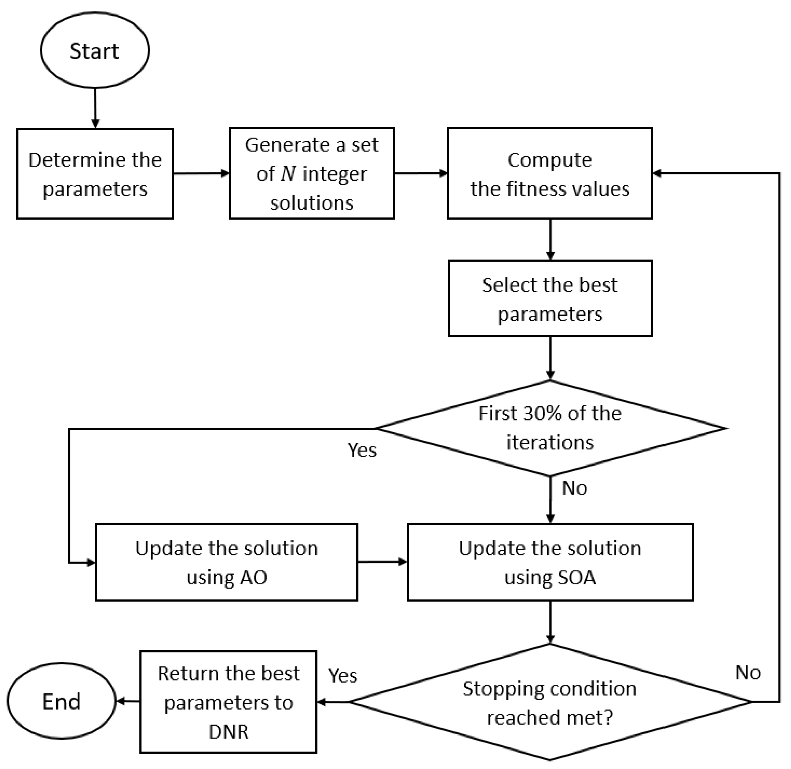
This study works to optimize DNR using an enhanced version of the SOA to produce a method called SOAAO. The workflow of the proposed method is presented in Figure 1. In the SOAAO method, the operators of the AO are used to improve the original SOA.
In detail, the AO operators are applied as a local search of the SOA to increase its ability to solve different optimization problems. This modification adds more flexibility to the SOAAO to explore the search domain and improve diversity. Then, the SOAAO is used to train the DNR method by optimizing its weight.
The SOAAO starts by declaring all the parameters, generating the initial solutions, and reading the dataset to prepare for the experiment steps. Then, the first stage of the SOA method searches for the best DNR weight; this weight is evaluated by mean square error (MSE) (see Equation (26)) to check its equality. This step is run to collect the initial fitness function values.
The next optimization steps update and evaluate all generated solutions. Here, the first 30% of iterations apply the operators of the AO (Equation (11)) to help the proposed method explore the search space. Then, in the remaining iterations, the SOA is employed to update the rest of the solution agents.
This sequence is repeated for the population until it reaches the stop criteria. Then, the best weight within the optimization process is selected and saved to obtain the final results.
M S E = 1 n i = 1 n ( b o i ( b c i ) 2
in which b o and b c are the real and target data, respectively. N is the data size. The MSE equation measures the main square error between the target and output data to select the best weights based on the smallest value. Algorithm 1 shows the pseudo-code of the proposed method.
Algorithm 1 SOAAO-DNR pseudo-code.
1:
Declare all the parameters used in the experiment.
2:
Initialize the population randomly.
3:
Compute the initial objective values.
4:
Select the best solution among the population.
5:
Initialize the iteration i = 0
6:
while (i < max iteration) do
7:
    Update the parameters of the optimization process such as random and control parameters.
8:
    if first 30% of the iteration then
9:
        Update the solution using parameters of the AO algorithm
10:
    else
11:
        Update the solution using parameters of the SOA algorithm.
12:
    end if
13:
    Pass the solution to train the DNR model.
14:
    Compute the objective value.
15:
    Save the best value.
16:
     i = i + 1
17:
end while
18:
Return the best DNR parameters.

4. Experimental Evaluation

4.1. Dataset Description

We used four datasets to consider the capability of the DNR-SOAAO model. They were collected from wind turbines in France between 2017 to 2020. Table 1 presents all their variables, which were recorded every ten minutes. In addition, the statistical values for the variables are listed in Table 2, including standard deviation, mean, minimum, and maximum. In our evaluation, the output values were normalized to be in the range [0, 1]. The experiment utilized 53491 continuous data as a time series. We used 42,792 data to train the model and the last 10,699 to test it.

4.2. Results and Discussion

To assess the quality of the DNR-SOAAO, we compared it to the original DNR model, as well as to several optimized DNR models using other optimization techniques, such as the genetic algorithm (GA), sine cosine algorithm (SCA), grey wolf optimizer (GWO), marine predators algorithm (MPA), traditional SOA, and traditional AO. We used four metrics, coefficient of determination R 2 , mean absolute error (MAE), root mean square error (RMSE), and mean relative absolute error (MRAE). All algorithms were applied in the same environment using MATLAB R2014b, “MS-Windows 10”, an “Intel Core-i7 CPU”, and 8GB of RAM. We used the same fitness evaluation number of 2500 for all algorithms. The parameter settings for the algorithms were the same as those listed in the original papers.
The results of all four evaluation indicators are presented in Table 3, Table 4, Table 5 and Table 6. In terms of RMSE, as listed in Table 3, the SOAAO recorded the best outcomes in three out of four datasets (DS2, DS3, and DS4). For DS1, the MPA obtained the best RMSE value (smallest RMSE), followed by GWO, the proposed SOAAO, PSO, GA, SOA, traditional DNR, and AO. In terms of MAE and MARE, the proposed SOAAO achieved the best results in both DS2 and DS3. The MPA obtained the best results in DS1, whereas the best MAE value in DS3 was obtained by the GWO, as shown in Table 4 and Table 5. These results indicate that the predicted wind power value is close to the target value.
Additionally, in terms of R 2 , the best results for all datasets were obtained by the proposed SOAAO method, as presented in Table 6. For more analysis, Figure 2 and Figure 3 show examples of QQ plots of the target value and the predicted value for two datasets—DS3 and DS4—respectively. The SOAAO achieved the best R 2 compared to all methods. This refers to the high correlation between the predicted wind power using the SOAAO and the target value, seen by most of the samples values following straight line. Therefore, from these results, it is clear that the combination of SOA and AO achieved better results than the traditional SOA and AO algorithms for all datasets. At the same time, the application of SOAAO with DNR obtained better results than traditional DNR. We can conclude that the optimization of DNR has significant impacts on its prediction performance.
To further ensure the quality of the proposed SOAAO compared to other optimization algorithms, we conducted the Friedman test, which is a well-known non-parametric statistical test that can be utilized to find differences between methods. The results are presented in Table 7. We can see that the SOAAO obtained the best value (smallest value) in three datasets (DS2, DS2, and DS4), whereas the GWO recorded the smallest value in the first dataset (DS1). This indicates the significantly improved performance of the proposed SOAAO over other models.
From the previous results, it can be noted that the developed SOAAO has a strong ability to discover the feasible region that contains the optimal parameters for the DNN. This enhances performance in wind power prediction. However, the SOAAO is still time consuming, especially with an increasing number of parameters.

5. Conclusions

In recent years, green power technologies have received wide attention. One of the most important green power resources is wind power. Thus, the estimation and prediction of wind power are necessary to plan effectively. To this end, this paper presented an alternative wind power time series prediction approach using an optimized dendritic neural regression (DNR) model. We utilized the recent developments of metaheuristics to train and optimize the traditional DNR model to enhance its forecasting capability. We proposed a new version of the seagull optimization algorithm (SOA) by employing the operators of the Aquila optimizer. The developed method, called SOAAO, was applied to train and optimize the parameters of a DNR model. We evaluated the DNR-SOAAO approach using four open-source datasets collected from real wind turbines located in France. To assess the quality of the SOAAO, we comparing it to other optimization algorithms to verify its performance using different evaluation indicators. Overall, the evaluation outcomes verified the competitive and efficient performance of the SOAAO compared to the original versions of the AO and SOA, as well as other well-known optimization algorithms. For instance, the SOAAO achieved the highest R 2 outcomes, of 0.95, 0.96, 0.95, and 0.91, for the four datasets. In future works, the SOAAO optimizer could be utilized for other applications, for example, image segmentation, data clustering, global optimization, and other optimization problems.

Author Contributions

Conceptualization, M.A.A.A.-q. and A.A.E.; methodology, M.A.A.A.-q. and A.A.E.; software, M.A.A.A.-q. and A.A.E.; validation, M.A.E. and A.H.S. formal analysis, M.A.E. and A.H.S.; investigation, M.A.A.A.-q. and A.A.E.; resources, M.A.A.A.-q.; data curation, A.A.E. and A.H.S.; writing—original draft preparation, M.A.A.A.-q., A.A.E. and A.H.S.; writing—review and editing, M.A.A.A.-q., A.A.E., M.A.E. and A.H.S.; visualization, A.A.E.; supervision, M.A.A.A.-q.; project administration, M.A.A.A.-q.; funding acquisition, M.A.A.A.-q. All authors have read and agreed to the published version of the manuscript.

Funding

This work was supported by National Natural Science Foundation of China (Grant No. 62150410434).

Data Availability Statement

The utilized datasets are available online as described in the paper.

Conflicts of Interest

All authors declare they have no conflict of interest.

References

  1. Zhao, X.; Wang, C.; Su, J.; Wang, J. Research and application based on the swarm intelligence algorithm and artificial intelligence for wind farm decision system. Renew. Energy 2019, 134, 681–697. [Google Scholar] [CrossRef]
  2. Wang, J.; Niu, T.; Lu, H.; Yang, W.; Du, P. A novel framework of reservoir computing for deterministic and probabilistic wind power forecasting. IEEE Trans. Sustain. Energy 2019, 11, 337–349. [Google Scholar] [CrossRef]
  3. Du, P.; Wang, J.; Yang, W.; Niu, T. Multi-step ahead forecasting in electrical power system using a hybrid forecasting system. Renew. Energy 2018, 122, 533–550. [Google Scholar] [CrossRef]
  4. Wang, J.; Du, P.; Niu, T.; Yang, W. A novel hybrid system based on a new proposed algorithm—Multi-Objective Whale Optimization Algorithm for wind speed forecasting. Appl. Energy 2017, 208, 344–360. [Google Scholar] [CrossRef]
  5. Jiang, P.; Yang, H.; Heng, J. A hybrid forecasting system based on fuzzy time series and multi-objective optimization for wind speed forecasting. Appl. Energy 2019, 235, 786–801. [Google Scholar] [CrossRef]
  6. Wang, D.; Luo, H.; Grunder, O.; Lin, Y. Multi-step ahead wind speed forecasting using an improved wavelet neural network combining variational mode decomposition and phase space reconstruction. Renew. Energy 2017, 113, 1345–1358. [Google Scholar] [CrossRef]
  7. Wang, Y.; Wang, J.; Wei, X. A hybrid wind speed forecasting model based on phase space reconstruction theory and Markov model: A case study of wind farms in northwest China. Energy 2015, 91, 556–572. [Google Scholar] [CrossRef]
  8. Zhao, J.; Guo, Z.H.; Su, Z.Y.; Zhao, Z.Y.; Xiao, X.; Liu, F. An improved multi-step forecasting model based on WRF ensembles and creative fuzzy systems for wind speed. Appl. Energy 2016, 162, 808–826. [Google Scholar] [CrossRef]
  9. Dong, Q.; Sun, Y.; Li, P. A novel forecasting model based on a hybrid processing strategy and an optimized local linear fuzzy neural network to make wind power forecasting: A case study of wind farms in China. Renew. Energy 2017, 102, 241–257. [Google Scholar] [CrossRef]
  10. Lahouar, A.; Slama, J.B.H. Hour-ahead wind power forecast based on random forests. Renew. Energy 2017, 109, 529–541. [Google Scholar] [CrossRef]
  11. Du, P.; Wang, J.; Guo, Z.; Yang, W. Research and application of a novel hybrid forecasting system based on multi-objective optimization for wind speed forecasting. Energy Convers. Manag. 2017, 150, 90–107. [Google Scholar] [CrossRef]
  12. Jiang, P.; Li, C.; Li, R.; Yang, H. An innovative hybrid air pollution early-warning system based on pollutants forecasting and Extenics evaluation. Knowl.-Based Syst. 2019, 164, 174–192. [Google Scholar] [CrossRef]
  13. Hao, Y.; Tian, C. The study and application of a novel hybrid system for air quality early-warning. Appl. Soft Comput. 2019, 74, 729–746. [Google Scholar] [CrossRef]
  14. Li, C.; Zhu, Z. Research and application of a novel hybrid air quality early-warning system: A case study in China. Sci. Total Environ. 2018, 626, 1421–1438. [Google Scholar] [CrossRef]
  15. Yang, W.; Wang, J.; Niu, T.; Du, P. A hybrid forecasting system based on a dual decomposition strategy and multi-objective optimization for electricity price forecasting. Appl. Energy 2019, 235, 1205–1225. [Google Scholar] [CrossRef]
  16. Niu, M.; Sun, S.; Wu, J.; Yu, L.; Wang, J. An innovative integrated model using the singular spectrum analysis and nonlinear multi-layer perceptron network optimized by hybrid intelligent algorithm for short-term load forecasting. Appl. Math. Model. 2016, 40, 4079–4093. [Google Scholar] [CrossRef]
  17. Li, G.; Shi, J. On comparing three artificial neural networks for wind speed forecasting. Appl. Energy 2010, 87, 2313–2320. [Google Scholar] [CrossRef]
  18. Jiang, P.; Liu, Z. Variable weights combined model based on multi-objective optimization for short-term wind speed forecasting. Appl. Soft Comput. 2019, 82, 105587. [Google Scholar] [CrossRef]
  19. Yin, H.; Ou, Z.; Huang, S.; Meng, A. A cascaded deep learning wind power prediction approach based on a two-layer of mode decomposition. Energy 2019, 189, 116316. [Google Scholar] [CrossRef]
  20. Du, P.; Wang, J.; Yang, W.; Niu, T. A novel hybrid model for short-term wind power forecasting. Appl. Soft Comput. 2019, 80, 93–106. [Google Scholar] [CrossRef]
  21. Zhu, J.; Su, L.; Li, Y. Wind power forecasting based on new hybrid model with TCN residual modification. Energy AI 2022, 10, 100199. [Google Scholar] [CrossRef]
  22. Huang, Q.; Wang, X. A Forecasting Model of Wind Power Based on IPSO–LSTM and Classified Fusion. Energies 2022, 15, 5531. [Google Scholar] [CrossRef]
  23. Huang, X.; Jiang, A. Wind Power Generation Forecast Based on Multi-Step Informer Network. Energies 2022, 15, 6642. [Google Scholar] [CrossRef]
  24. Liao, S.; Tian, X.; Liu, B.; Liu, T.; Su, H.; Zhou, B. Short-Term Wind Power Prediction Based on LightGBM and Meteorological Reanalysis. Energies 2022, 15, 6287. [Google Scholar] [CrossRef]
  25. Hanifi, S.; Lotfian, S.; Zare-Behtash, H.; Cammarano, A. Offshore Wind Power Forecasting—A New Hyperparameter Optimisation Algorithm for Deep Learning Models. Energies 2022, 15, 6919. [Google Scholar] [CrossRef]
  26. Ji, J.; Dong, M.; Lin, Q.; Tan, K.C. Forecasting Wind Speed Time Series Via Dendritic Neural Regression. IEEE Comput. Intell. Mag. 2021, 16, 50–66. [Google Scholar] [CrossRef]
  27. Song, Z.; Tang, Y.; Ji, J.; Todo, Y. Evaluating a dendritic neuron model for wind speed forecasting. Knowl.-Based Syst. 2020, 201, 106052. [Google Scholar] [CrossRef]
  28. Tang, C.; Todo, Y.; Ji, J.; Lin, Q.; Tang, Z. Artificial immune system training algorithm for a dendritic neuron model. Knowl.-Based Syst. 2021, 233, 107509. [Google Scholar] [CrossRef]
  29. Schuman, C.D.; Potok, T.E.; Patton, R.M.; Birdwell, J.D.; Dean, M.E.; Rose, G.S.; Plank, J.S. A survey of neuromorphic computing and neural networks in hardware. arXiv 2017, arXiv:1705.06963. [Google Scholar]
  30. Ji, J.; Tang, C.; Zhao, J.; Tang, Z.; Todo, Y. A survey on dendritic neuron model: Mechanisms, algorithms and practical applications. Neurocomputing 2022, 489, 390–406. [Google Scholar] [CrossRef]
  31. Tang, Z.; Tamura, H.; Kuratu, M.; Ishizuka, O.; Tanno, K. A model of the neuron based on dendrite mechanisms. Electron. Commun. Jpn. (Part III Fundam. Electron. Sci.) 2001, 84, 11–24. [Google Scholar] [CrossRef]
  32. Tang, Z.; Kuratu, M.; Tamura, H.; Ishizuka, O.; Tanno, K. A neuron model based on dendritic mechanism. IEICE 2000, 83, 486–498. [Google Scholar]
  33. Yu, Y.; Wang, Y.; Gao, S.; Tang, Z. Statistical modeling and prediction for tourism economy using dendritic neural network. Comput. Intell. Neurosci. 2017, 2017, 7436948. [Google Scholar] [CrossRef] [Green Version]
  34. Tang, Y.; Song, Z.; Zhu, Y.; Hou, M.; Tang, C.; Ji, J. Adopting a dendritic neural model for predicting stock price index movement. Expert Syst. Appl. 1176. [Google Scholar]
  35. Song, Z.; Tang, C.; Ji, J.; Todo, Y.; Tang, Z. A simple dendritic neural network model-based approach for daily PM2. 5 concentration prediction. Electronics 2021, 10, 373. [Google Scholar] [CrossRef]
  36. Dong, M.; Tang, C.; Ji, J.; Lin, Q.; Wong, K.C. Transmission trend of the COVID-19 pandemic predicted by dendritic neural regression. Appl. Soft Comput. 2021, 111, 107683. [Google Scholar] [CrossRef]
  37. Qian, X.; Tang, C.; Todo, Y.; Lin, Q.; Ji, J. Evolutionary Dendritic Neural Model for Classification Problems. Complexity 2020, 2020, 1–13. [Google Scholar] [CrossRef]
  38. Egrioglu, E.; Baş, E.; Chen, M.Y. Recurrent Dendritic Neuron Model Artificial Neural Network for Time Series Forecasting. Inf. Sci. 2022, 607, 572–584. [Google Scholar] [CrossRef]
  39. Dhiman, G.; Kumar, V. Seagull optimization algorithm: Theory and its applications for large-scale industrial engineering problems. Knowl.-Based Syst. 2019, 165, 169–196. [Google Scholar] [CrossRef]
  40. Xian, S.; Chen, K.; Cheng, Y. Improved seagull optimization algorithm of partition and XGBoost of prediction for fuzzy time series forecasting of COVID-19 daily confirmed. Adv. Eng. Softw. 2022, 173, 103212. [Google Scholar] [CrossRef]
  41. Long, W.; Jiao, J.; Liang, X.; Xu, M.; Tang, M.; Cai, S. Parameters estimation of photovoltaic models using a novel hybrid seagull optimization algorithm. Energy 2022, 249, 123760. [Google Scholar] [CrossRef]
  42. Xu, L.; Mo, Y.; Lu, Y.; Li, J. Improved Seagull Optimization Algorithm Combined with an Unequal Division Method to Solve Dynamic Optimization Problems. Processes 2021, 9, 1037. [Google Scholar] [CrossRef]
  43. Jagannathan, P.; Gurumoorthy, S.; Stateczny, A.; Divakarachar, P.B.; Sengupta, J. Collision-Aware Routing Using Multi-Objective Seagull Optimization Algorithm for WSN-Based IoT. Sensors 2021, 21, 8496. [Google Scholar] [CrossRef] [PubMed]
  44. Yu, H.; Qiao, S.; Heidari, A.A.; Bi, C.; Chen, H. Individual Disturbance and Attraction Repulsion Strategy Enhanced Seagull Optimization for Engineering Design. Mathematics 2022, 10, 276. [Google Scholar] [CrossRef]
  45. Panagant, N.; Pholdee, N.; Bureerat, S.; Kaen, K.; Yıldız, A.R.; Sait, S.M. Seagull optimization algorithm for solving real-world design optimization problems. Mater. Test. 2020, 62, 640–644. [Google Scholar] [CrossRef]
  46. Dhiman, G.; Singh, K.K.; Soni, M.; Nagar, A.; Dehghani, M.; Slowik, A.; Kaur, A.; Sharma, A.; Houssein, E.H.; Cengiz, K. MOSOA: A new multi-objective seagull optimization algorithm. Expert Syst. Appl. 2021, 167, 114150. [Google Scholar] [CrossRef]
  47. Wang, Z.; Geng, Z.; Fang, X.; Tian, Q.; Lan, X.; Feng, J. The Optimal and Economic Planning of a Power System Based on the Microgrid Concept with a Modified Seagull Optimization Algorithm Integrating Renewable Resources. Appl. Sci. 2022, 12, 4743. [Google Scholar] [CrossRef]
  48. Xia, Q.; Ding, Y.; Zhang, R.; Zhang, H.; Li, S.; Li, X. Optimal Performance and Application for Seagull Optimization Algorithm Using a Hybrid Strategy. Entropy 2022, 24, 973. [Google Scholar] [CrossRef]
  49. Liu, X.; Li, G.; Shao, P. A Multi-Mechanism Seagull Optimization Algorithm Incorporating Generalized Opposition-Based Nonlinear Boundary Processing. Mathematics 2022, 10, 3295. [Google Scholar] [CrossRef]
  50. Abualigah, L.; Yousri, D.; Abd Elaziz, M.; Ewees, A.A.; Al-Qaness, M.A.; Gandomi, A.H. Aquila optimizer: A novel meta-heuristic optimization algorithm. Comput. Ind. Eng. 2021, 157, 107250. [Google Scholar] [CrossRef]
  51. Al-qaness, M.A.; Ewees, A.A.; Fan, H.; AlRassas, A.M.; Abd Elaziz, M. Modified aquila optimizer for forecasting oil production. Geo-Spat. Inf. Sci. [CrossRef]
  52. Dahou, A.; Al-qaness, M.A.; Abd Elaziz, M.; Helmi, A. Human activity recognition in IoHT applications using arithmetic optimization algorithm and deep learning. Measurement 2022, 199, 111445. [Google Scholar] [CrossRef]
  53. Fatani, A.; Dahou, A.; Al-Qaness, M.A.; Lu, S.; Elaziz, M.A. Advanced feature extraction and selection approach using deep learning and Aquila optimizer for IoT intrusion detection system. Sensors 2021, 22, 140. [Google Scholar] [CrossRef] [PubMed]
  54. Xing, Q.; Wang, J.; Lu, H.; Wang, S. Research of a novel short-term wind forecasting system based on multi-objective Aquila optimizer for point and interval forecast. Energy Convers. Manag. 2022, 263, 115583. [Google Scholar] [CrossRef]
  55. Abou El-Ela, A.A.; El-Sehiemy, R.A.; Shaheen, A.M.; Shalaby, A.S. Aquila Optimization Algorithm for Wind Energy Potential Assessment Relying on Weibull Parameters Estimation. Wind 2022, 2, 617–635. [Google Scholar] [CrossRef]
  56. Khamees, A.K.; Abdelaziz, A.Y.; Eskaros, M.R.; El-Shahat, A.; Attia, M.A. Optimal Power Flow Solution of Wind-Integrated Power System Using Novel Metaheuristic Method. Energies 2021, 14, 6117. [Google Scholar] [CrossRef]
  57. Zhou, T.; Gao, S.; Wang, J.; Chu, C.; Todo, Y.; Tang, Z. Financial time series prediction using a dendritic neuron model. Knowl.-Based Syst. 2016, 105, 214–224. [Google Scholar] [CrossRef]
Figure 1. The proposed method.
Energies 15 09261 g001
Figure 2. Results on DS3.
Energies 15 09261 g002
Figure 3. Results on DS4.
Energies 15 09261 g003
Table 1. Dataset variables: standard deviation (Std), maximum (Max), minimum (Min).
No.TypeField
1First anemometer on the nacelleAverage
2 Min
3 Max
4 Std
5Second anemometer on the nacelleAverage value
6 Min
7 Max
8 Std
9Average wind speedAverage
10 Min
11 Max
12 Std
14Absolute wind directionAverage value
15 Min
16 Max
17 Std
Table 2. Target data details and statistics.
MeanMinMaxStd
R807110.20520010.23250
R807210.16580010.20560
R807360.17440010.22170
R807900.18550010.22430
Table 3. RMSE results.
RMSESOAAOSOAAOMPAPSOGAGWODNR
DS10.043170.060300.125880.041140.047710.054260.041600.06545
DS20.030100.053980.138340.030550.033400.041250.034290.06923
DS30.037810.065320.061350.044040.048750.042430.038490.08375
DS40.053460.066480.068970.054900.060270.059930.057210.08730
Table 4. MAE results.
SOAAOSOAAOMPAPSOGAGWODNR
DS10.030800.040420.092590.025820.032630.035850.027960.04232
DS20.019270.036190.102270.019630.021900.027730.021810.04609
DS30.021680.043310.034620.025760.029830.024740.020630.05871
DS40.026430.037980.044940.030580.036490.034300.031340.05604
Table 5. MARE results.
SOAAOSOAAOMPAPSOGAGWODNR
DS10.143420.180120.424730.117170.150160.153340.148330.16938
DS20.095280.178410.530940.100840.109630.129520.104400.21824
DS30.124270.216420.161300.137360.153150.130980.111090.29954
DS40.151860.187130.246040.159870.187750.181480.161160.28551
Table 6. R2 results.
RMSESOAAOSOAAOMPAPSOGAGWODNR
DS10.952260.882230.457160.951990.938650.921710.949220.87618
DS20.966880.867300.235290.965880.958860.941440.954620.81020
DS30.956020.849550.881160.936310.926490.945440.952380.71161
DS40.914710.863710.867470.909940.895670.899610.897290.75190
Table 7. The results of Friedman test.
SOAAOSOAAOMPAPSOGAGWODNR
DS12.895.117.782.783.894.672.116.78
DS22.445.117.442.673.225.333.116.67
DS31.786.226.444.004.113.672.337.44
DS42.225.566.782.444.334.113.117.44
Publisher’s Note: MDPI stays neutral with regard to jurisdictional claims in published maps and institutional affiliations.

