Article

Dynamic DNR and Solar PV Smart Inverter Control Scheme Using Heterogeneous Multi-Agent Deep Reinforcement Learning

Department of Electrical Engineering, Soongsil University, Seoul 06978, Republic of Korea
*
Author to whom correspondence should be addressed.
Energies 2022, 15(23), 9220; https://doi.org/10.3390/en15239220
Submission received: 30 October 2022 / Revised: 24 November 2022 / Accepted: 1 December 2022 / Published: 5 December 2022

Abstract

:
The conventional volt-VAR control (VVC) in distribution systems has limitations in solving the overvoltage problem caused by massive solar photovoltaic (PV) deployment. As an alternative method, VVC using solar PV smart inverters (PVSIs) has come into the limelight, which can respond quickly and effectively to solve the overvoltage problem by absorbing reactive power. However, the network power loss, that is, the sum of line losses in the distribution network, increases with reactive power. Dynamic distribution network reconfiguration (DNR), which hourly controls the network topology by controlling sectionalizing and tie switches, can also solve the overvoltage problem and reduce network loss by changing the power flow in the network. In this study, to improve the voltage profile and minimize the network power loss, we propose a control scheme that integrates the dynamic DNR with volt-VAR control of PVSIs. The proposed control scheme is practically usable for three reasons: Primarily, the proposed scheme is based on a deep reinforcement learning (DRL) algorithm, which does not require accurate distribution system parameters. Furthermore, we propose the use of a heterogeneous multiagent DRL algorithm to control the switches centrally and PVSIs locally. Finally, a practical communication network in the distribution system is assumed. PVSIs only send their status to the central control center, and there is no communication between the PVSIs. A modified 33-bus distribution test feeder reflecting the system conditions of South Korea is used for the case study. The results of this case study demonstrates that the proposed control scheme effectively improves the voltage profile of the distribution system. In addition, the proposed scheme reduces the total power loss in the distribution system, which is the sum of the network power loss and curtailed energy, owing to the voltage violation of the solar PV output.

1. Introduction

Conventional control devices for volt/VAR control (VVC) in distribution systems are on-load tap changers (OLTC) and capacitor banks (CB) [1]. Currently, distribution systems have more control functions to support the rapidly increasing penetration of renewable energy. For example, dynamic distribution network reconfiguration (DNR) that controls sectionalizing and tie switches reduces network power loss by changing power flow [2,3,4]. It is a cost-effective method to increase the hosting capacity of solar photovoltaics (PV) [5,6]. The distribution system operator (DSO) controls these devices to maintain the voltage level in the normal operating range and operate the distribution system economically. Another important control entity is the smart inverter installed in the solar PV generator. The PV smart inverter (PVSI) is installed at the bus that suffers from the overvoltage problem, and it can absorb and provide reactive power. Therefore, VVC using PVSI shows a better performance than traditional VVC methods using OLTC or CB. Cooperative control schemes using both PVSI and dynamic DNR further improve the performance of voltage regulation and network power loss [7].
Previous studies on VVC and dynamic DNR can be categorized into model-based and model-free algorithms. The optimization framework of model-based approaches is generally non-convex because of the non-linearity of the power system. Therefore, these non-convex optimization problems have been converted to those of convex optimization [4,8], mixed-integer linear programming (MILP) [3,9], mixed-integer quadratic programming (MIQP) [10], and mixed-integer second-order cone programming (MISOCP) [11,12]. Because model-based approaches are based on an optimization framework, they have shown good performance. However, these approaches are difficult to apply to real distribution systems. This is because model-based approaches heavily depend on a specific model, which requires accurate distribution system parameters such as load, solar PV output, and impedance of power lines.
To overcome the limitations of model-based approaches, model-free algorithms, that is data-driven approaches, have been investigated [13,14,15,16,17]. In [13], the authors formulated dynamic DNR as a Markov decision process (MDP) and trained a deep Q-network (DQN) based on historical operational datasets. They also proposed a data-augmentation method to generate synthetic training data using a Gaussian process. A two-stage deep reinforcement learning (DRL) method consisting of offline and online stages was proposed to improve the voltage profile using PVSIs [16]. In our previous work [18], we developed a DQN-based dynamic DNR algorithm for energy loss minimization.
Furthermore, model-free algorithms can control different devices in a coordinated manner using multi-agent reinforcement learning. In [19], a multi-agent deep Q-network based algorithm that controls CB, voltage regulators, and PVSIs by interacting with the distribution system was proposed. Different types of devices were modeled as independent agents. Through this mechanism, independent agents share the same state and reward. However, they also adopt a centralized control scheme that requires heavy communication to obtain global information between agents. In [20], a centralized off-policy maximum entropy reinforcement learning algorithm was proposed using a voltage regulator, CB, and OLTC. Their proposed algorithm showed good voltage violation and power loss performance with limited communication among agents. However, communication between agents is still required, despite the reduced amount of communication.
Hybrid approaches that combine model-based and model-free methods have also been investigated [12,21]. In [21], a two-timescale control algorithm was proposed. On a slow timescale, the operations of OLTC and CBs are determined using the MISOCP-based optimal power flow method. In contrast, a DRL algorithm is applied to control the reactive power of PVSIs locally on a fast timescale. Similarly, a two-timescale and a hybrid of model-based and model-free methods for VVC were proposed in [12]. Their proposed algorithm controls shunt capacitors hourly using the DRL algorithm and PVSIs in seconds, using an optimization framework to improve the voltage profile. However, these approaches have the same limitations as model-based algorithms that involve optimization problems.
Most VVC control schemes operate in a centralized manner, even with a data-driven approach. Centralized control schemes require communication between the central control center and field devices, such as PVSIs, resulting in an increase in the amount of communication and computational complexity. In addition, DSO cannot fully control PVSIs when solar PVs are owned by PV generation companies. Therefore, centralized control schemes are not practical for the real operation of distribution systems.
In this paper, we propose a heterogeneous multiagent DRL (HMA-DRL) algorithm for voltage regulation and network loss minimization in distribution systems, which combines the central control of dynamic DNR and local control of PVSIs (Centralized VVC normally controls OLTC and CBs. However, recent research shows that dynamic DNR further improves the performance in terms of energy savings [7]. Therefore, in this study, we chose dynamic DNR as the main control method for the DSO using a switch entity because dynamic DNR can be used on top of a traditional VVC using OLTC and CBs). We use DRL algorithms for central and local controls, but they have different states, actions, and rewards, that is, heterogeneous DRL, because their ownership types are different. Through a case study using a modified 33-bus distribution test feeder, the proposed HMA-DRL algorithm shows the best performance in terms of total power loss with no voltage violation among model-free methods. The total power loss is the sum of the curtailed energy, owing to voltage violations and network power loss. The main contribution of this work is the practical applicability of the proposed HMA-DRL algorithm. These are listed as follows:
  • Control authority: The two main control entities (switches and PVSIs) are owned by different parties in general. Typically, DSO and PV generation companies have switches and PVSIs, respectively. Therefore, in this study, we give their control authority to the owners. The agent located at the central control center (CCC) operates switches by the DSO, i.e., dynamic DNR, to mainly minimize network power loss. On the other hand, the agents located at PVSIs control the reactive power of the PVSIs to maintain the voltage level in the normal range by the PV generation companies.
  • Practical communication requirement: Each agent has different levels of information because of the different control authorities. The DSO can monitor PVSI’s active and reactive power output of solar PV as well as the overall status of the distribution system. Therefore, the agent at CCC can use this information. In contrast, agents at PVSIs can only observe their own buses. Therefore, the proposed HMA-DRL algorithm does not require a communication link for the control signal from CCC to PVSIs. Instead, it only requires a feedback link from PVSIs to CCC (a feedback link for reporting a simple measurement reading can use a public communication link with encryption; however, the communication link for the control signal requires a high level of security, such as private communication, owing to its importance) and the control signal from CCC to switches (We assume that a communication link between the CCC and switches already exists because the DSO owns switches and takes charge of its operation). Because the control signal to each PVSI requires a higher security level than simple status feedback, we believe that this assumption on communication requirements is practical for distribution systems.
  • Heterogeneous multi-agent DRL: A heterogeneous multi-agent DRL algorithm is applied for voltage regulation and dynamic DNR to remove the dependency of the distribution system parameters. We modeled the state, action, and reward of the MDP for each agent, the MDP of the dynamic DNR with the overall status of the distribution system, while the MDP of the voltage regulation at PVSI utilizes local measurements. In this manner, the agent at CCC and agents at PVSIs learn an optimal policy that complements each other because each reward results from their simultaneous combined action.
The remainder of this paper is organized as follows. In Section 2, we first describe the system model and formulate the optimization problem. In Section 3, the proposed HMA-DRL algorithm is described. After demonstrating the performance of the proposed algorithm in Section 4, we conclude this paper in Section 5.

2. System Model and Problem Formulation

2.1. System Model

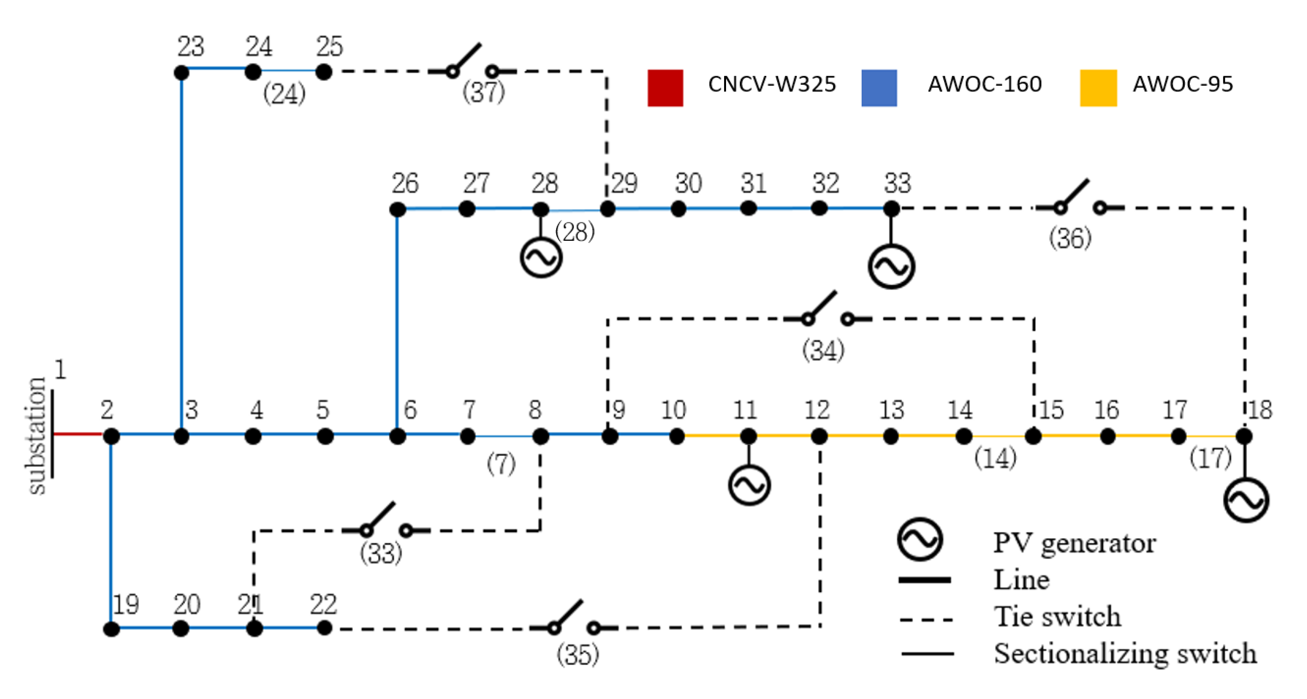
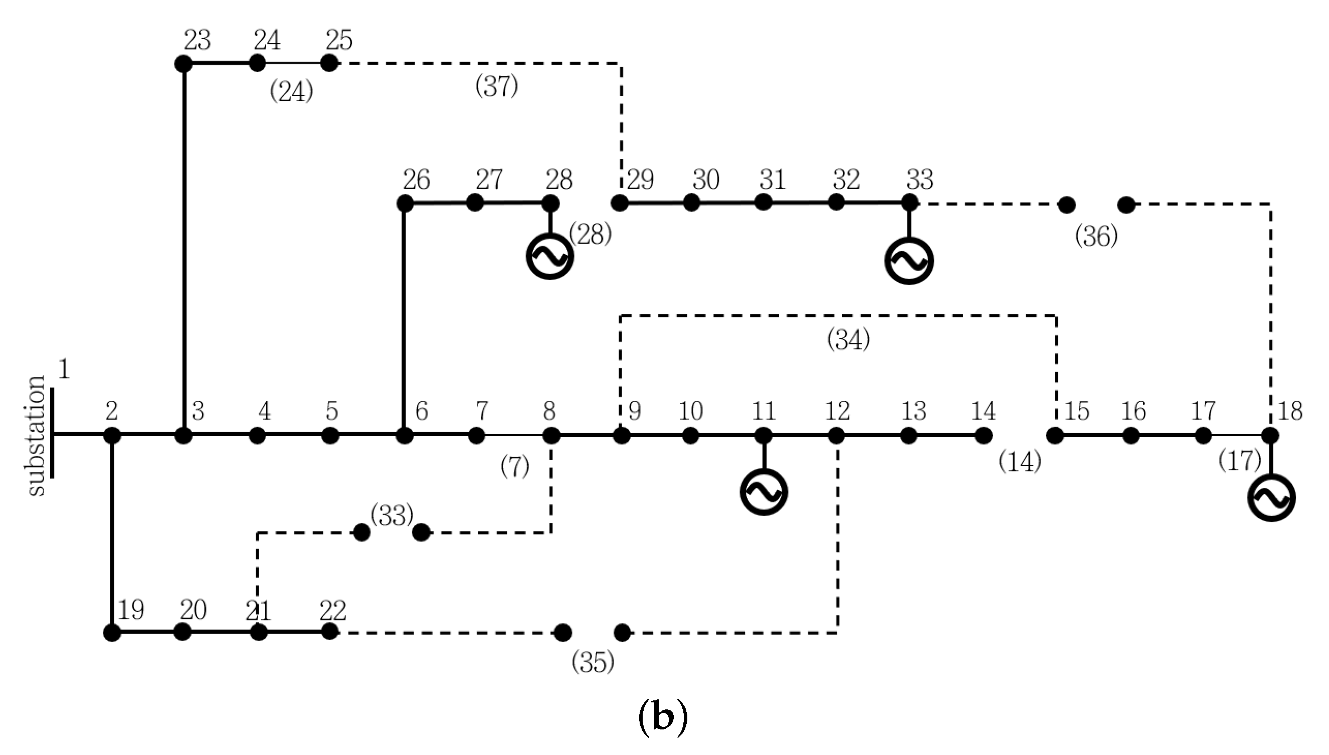
We consider a radial distribution system as shown in Figure 1. The distribution system has several control units, such as sectionalizing and tie switches, OLTC, CBs, and solar PVs. Smart inverters operate all the solar PVs in this system. The control entities in this study are switches and PVSIs. The sets of buses and power lines are denoted as N and E , respectively. We assume that bus 1 is at the substation. We denote the set of buses with installed solar PV generators as K . Each day is divided by the control period and is denoted by a period set as T = { 1 , 2 , , T } and the time index as t. The phasor voltage and current in bus n at time t are V t n and I t n , respectively. Their magnitudes and phases angle are represented by | V t n | , | I t n | and δ t n , respectively. The net active power and reactive power in bus n at time t are represented by P t n and Q t n , respectively.
The voltage and current can be obtained by solving the power flow equations. At bus n, P n and Q n are computed as
P n = V n m = 1 N V m G m n cos ( δ n δ m ) + B m n sin ( δ n δ m ) ,
Q n = V n k = 1 N V m G m n sin ( δ n δ m ) B m n cos ( δ n δ m ) .
The DSO accounts for the stable and reliable operation of the distribution system. In this study, the main control entity of the DSO is switches to operate the distribution system reliably. When a switch takes action, i.e., opens or closes, the topology of the distribution system changes, i.e., dynamic DNR. Therefore, we assume that the DSO centrally controls every switch, and the status information of the system is delivered to the control center. The DSO controls switches as long as the distribution system forms a radial network topology.
Another control entity is PVSIs, which have two control options: centralized and local. In centralized control of PVSIs, the DSO obtains information on the solar PV output and sends a control signal to the PVSI. This approach can achieve an optimal operation from a global perspective. However, this is not practical because solar PV owners should provide complete control to the DSO, and a reliable and secure communication channel is required between them. Therefore, in this study, we focus on the local control of PVSIs. We assume that a PVSI installed on bus k can only observe local information, i.e., V t k , P t k and Q t k , and take action by itself, which is a more practical assumption.
Note that a feedback link exists between the solar PV generators, and the CCC from solar PV generators to CCC exists. This link requires a low level of security because it only delivers the status of the PVSIs to the CCC. This link can be a public link, i.e., the Internet, with encryption, rather than a private link. This is a realistic assumption for a communication network in the distribution systems.

2.2. Centralized Optimization

In this section, we describe the role of the DSO as an optimization framework. Stable and reliable operation of the distribution system is the first requirement of a DSO. As long as this requirement is fulfilled, the DSO wants to operate the distribution system economically. The two control variables in this optimization framework are the switch status and the reactive power outputs of the PVSIs. Let j t o denote a binary variable representing the status of switch located in line o at time t. If the switch is closed, its value is one. Otherwise, it is 0. The reactive power output of the PVSI installed on bus k at time t is Q t P V , k . We formulate the optimization framework of the DSO as follows:
( C ) min { j t o } t , { Q t P V , k } t t T e E I t e 2 R e
subject to ( 1 ) , ( 2 ) ,
V ̲ V t n V ¯ , n N , t T
I t e I e ¯ , e E , t T
j t A , t T
t T o O j t o j t 1 o N ¯ S W
Q t P V , k ( S P V , k ) 2 ( P t P V , k ) 2 , n K , t T
The objective function of the problem ( C ) is to minimize the network loss in the distribution system while maintaining the distribution system constraints.
The distribution system constraints are given by Equations (4a) and (4b), respectively. In other words, the DSO should maintain all voltages and currents in the system within the regulation range (Power lines near the substation have more capacity than those at the end of feeders in the distribution system. Therefore, power lines located near the substation have a higher current flow limit. A detailed specification of power lines is given in Section 4.1). One of the major constraints of dynamic DNR is that the distribution system remains to operate in a radial topology despite switching actions. Let j t and A denote a vector of the switch status and a feasible set of switching actions that guarantees the radial topology of the distribution system, respectively. Therefore, Equation (4c) describes the radial constraint of the distribution system. A feasible set for the radial constraint can be made using the spanning tree characteristics [9]. When the topology created by j t satisfies the following conditions, j t is a member of A . That is j t = [ j t 1 , j t 2 , , j t o , , j t | O | ] A :
j t o = b t m n + b t n m
m N ( n ) b t n m = 1 , n 2
where N ( n ) and b t n m are the set of all buses directly connected to bus n and a binary variable whose value is 1 if bus m is the parent of bus n and 0, otherwise, respectively.
Because switching actions reduce the lifespan of switches, we add a constraint of maximum switching numbers per day, as shown in Equation (4d). The final constraint, that is, Equation (4e), describes the reactive power output of a PVSI. Its maximum output is bounded by the capacity of the PVSI S P V , k and the current real power output of the PV P t P V , k [22].
The problem ( C ) is not a convex optimization problem because of the non-linearity of the power flow equations and integer control variables. In addition, it requires a high level of security communication because the DSO sends control signals (reactive power output) to the PVSIs. Finally, the DSO can solve this problem by knowing the distribution system parameters, such as power line impedance, load, and solar PV output. Therefore, we propose using a model-free algorithm to overcome these limitations.

3. Heterogeneous Multi-Agent DRL Algorithm

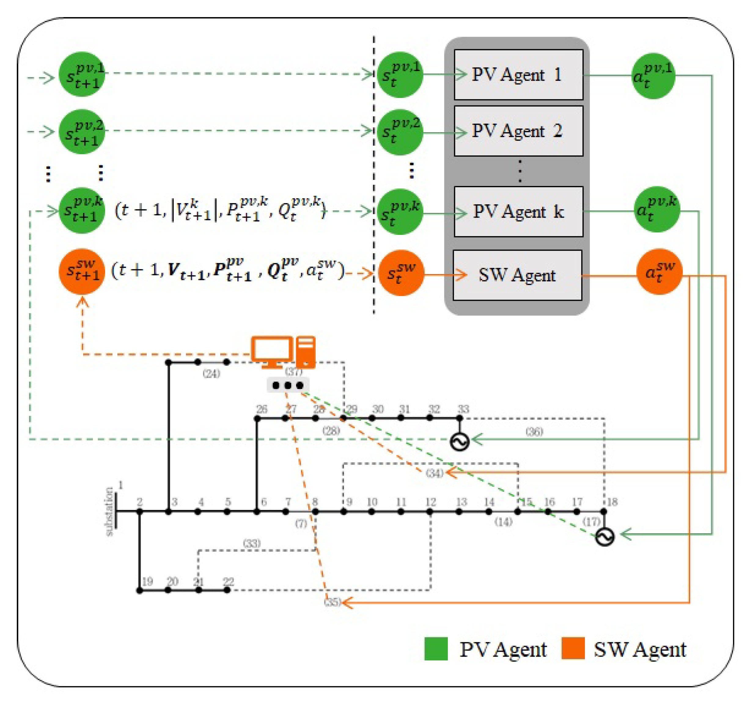
We propose a HMA-DRL algorithm for voltage regulation and network loss minimization in distribution systems that combines the central control of dynamic DNR and local control of PVSI. Figure 2 shows the framework of the proposed HMA-DRL algorithm. The proposed HMA-DRL algorithm divides the control entities into two main parts: an agent at CCC (SW agent) and agents at PVSIs (PVSI agent). The two different agents operate independently. In central control, the DSO controls the switches to minimize network loss while maintaining the radial constraint. To this end, the DSO monitors the real power and reactive power of buses and obtains voltage and current through power flow calculations (Recent research has shown that machine learning-based models can approximate the power flow without distribution network parameters [23,24]). In local control, PVSIs control their reactive power output to avoid an overvoltage problem at the bus. The agents at PVSIs only know their own active power output and voltage level at the bus.

3.1. Multi-Agent Markov Decision Process

To train agents in a cooperative manner, we define a multi-task decision-making problem as a multi-agent MDP. The multi-agent system in this work is a heterogeneous multi-agent system that has different MDPs for different types of agents [25]. The agent at CCC and agents at PVSIs have different types of agents because their ability to obtain information and control entities are different. Therefore, the agent at CCC and agents at PVSIs independently learn their policies, while other agents are regarded as part of the environment [26]. The multi-agent MDP is composed of ( X , S , A , { R x } x , P , γ ), where (i) X and x denote a set of agents and their indices, respectively. (ii) S = { S x } x is the joint space of state. (iii)  A = { A x } x denotes the joint action space of the agents. (iv) R x ( s x , a x ) = E [ R t + 1 | S t = s x , A t = a x ] denotes the expected local reward of agent x received after the state transition. (v) P : S × A × S [ 0 , 1 ] is the state transition probability, and (vi) γ [ 0 , 1 ] is a discount factor.
Each agent takes an action moving to a new state and receives a reward. The process ends when the terminal state is reached. Through these processes, the sum of the discounted local reward G t x of agent x at t is calculated as follows:
G t x = k = 0 γ k R t + k + 1 . x
The goal of MDP is to find a policy π that maximizes G t x . A policy π x ( a x | s x ) = P [ A t = a x | S t = s x ] is the probability of choosing an action a x in a given state s x . If the agents are the agent at CCC and agents at PVSIs, x is set as S W and P V , respectively.

3.2. MDP for Agent at CCC

The agent located at the CCC controls the open and close actions of switches, that is, dynamic DNR, because this action requires global information to maintain the radial topology of the distribution system. We define the state, action, and reward of this agent to minimize the sum of the network power losses in the distribution system while maintaining the voltage and current in the normal range.

3.2.1. State

We assume that the agent at the CCC can efficiently estimate the state of the distribution system, that is, the voltage of each bus, and obtain the output of PVSIs, including active and reactive power, through a feedback link (Each agent at PVSI sends its active and reactive power to the DSO every hour because the agent at DSO control switches status hourly. The latency requirement of this data is less than five seconds [27]). The state of MDP at t is defined as the time, voltages of all buses, real power outputs of PVSIs, reactive power outputs of PVSIs at t 1 , which are previous actions of PVSIs, and switching status at t 1 , that is, the previous action of the agent at the CCC. It is defined as
s t S W = ( t , V t , P t PV , Q t 1 PV , a t 1 S W ) .
We put previous actions into the current state because the agent at CCC understands the other agents’ actions, resulting in a better choice of action at the current time.

3.2.2. Action

For the agent at CCC, an action at t is the opening and closing of each switch, that is, a t S W = j t . After taking action, the topology of the distribution system changes. As the set of feasible actions A is already defined, the agent takes action in the set. In this manner, the radial constraint of the optimization problem, that is, Equation (4c), is fulfilled by setting a t S W A .

3.2.3. Reward

Because the MDP does not easily have constraints, we model the reward as a combination of the objective function and constraints of problem ( C ) . The reward consists of three parts: voltage violation and power loss v p t S W , current violation c v t S W , and penalty for frequent switching actions. That is
r t + 1 S W = v p t + 1 S W + c v t + 1 S W w s w · o O j t o j t 1 o .
We select the first two reward terms, v p t S W and c v t S W as step functions to effectively train the agent. From the point of problem ( C ) view, we model v p t S W for the network loss minimization and voltage violation, that is, Equations (3) and (4a), and is given as
v p t + 1 S W = 100 , if V ̲ V t n V ¯ , n N and l t D N R < l t 0 , if V ̲ V t n V ¯ , n N and l t D N R l t 100 , otherwise .
The agent at CCC obtains a positive reward when the network loss of the new topology is less than that of the initial topology without any voltage violation. The agent receives a negative reward for the voltage violation. Therefore, the agent preferentially avoids any voltage violation.
Next, c v t S W is modeled to imply a current violation, as shown in Equation (4b). It is
c v t + 1 S W = 0 , if I t e I e ¯ , e E 500 , otherwise .
When a current violation occurs in the distribution system, the agent at CCC receives a highly negative reward. Note that the reason for the time index t + 1 is that the agent receives a reward based on the outcome of its action at t. The last term corresponds directly to Equation (4d). Frequent switching action are not preferred. We put a negative reward per switching action and weight w on the hyperparameter adjusted by the DSO.
Note that the objective function and all the constraints in the problem ( C ) are included in this MDP formulation except the reactive power constraint, that is, Equation (4e). This is because the DSO cannot control the reactive power of PVSIs. Therefore, the MDP formulation for PVSIs includes this constraint.

3.3. MDP for Agents at PVSIs

Agents located at PVSIs operate in a distributed manner because they have no global information. They control their reactive power using only the local information. The objective of these agents is to keep their bus voltage stable rather than minimizing the sum of network power losses. This is because obtaining the sum of network power losses is not possible without global information.

3.3.1. State

Considering the condition that PVSIs can observe only their generation profile, we define the state of agent k as current time t, voltage magnitude of the bus that PVSI installed as | V t k | , real power output of PVSI as P t P V , k at the current time, and reactive power output of PVSI at the previous time as Q t 1 P V , k . That is,
s t P V , k = ( t , | V t k | , P t P V , k , Q t 1 P V , k ) .

3.3.2. Action

The possible actions of the PVSI are its reactive power output. By controlling the reactive power, the curtailed energy of the active power output can be avoided, that is, by maintaining its voltage level in a stable range. The maximum reactive power output is bounded by the active power output and capacity of the inverter, as expressed in Equation (4e). For example, when the output of a PVSI is 0.9 p.u., the maximum reactive power output of the smart inverter is 1 0 . 9 2 = 0.4359 p.u. Therefore, we set the control range of reactive power in this case study as 0.4 Q t P V , k 0.4 (In the case study, we use real solar PV output data from Yeongam, South Korea [28]. These data show that the PV output peak of 0.93 p.u. occurred in March, so the PVSI can absorb reactive power up to 1 0 . 93 2 = 0.37 p.u. without over-sizing the PVSI. Therefore, the proposed HMA-DRL algorithm has almost no issue with this reactive power margin. However, in case of the PV output peak is 1 p.u., it is recommended to install a power conditioning system (PCS) with a 10% margin, i.e., 1.1 p.u., to use voltage regulation algorithms [29]). We define action as the difference in reactive power outputs between t 1 and t in a discrete manner. That is,
a t P V , k = Q t P V , k Q t 1 P V , k = Δ Q t P V , k .
Note that each action is constrained by reactive power limit as shown in Equation (4e).

3.3.3. Reward

Because the agents at PVSIs try to minimize the curtailed energy of their active power, the objective of agents at PVSIs is to maintain their bus voltage stable. In addition, when there is no voltage violation, PVSIs help reduce the network power loss. We define the reward as a penalty for the severity of voltage violation, in case of voltage violation. The reward in the no voltage violation condition is set as the negative of the square of the apparent power. Because the apparent power and current injection, i.e., ( I t k = ( S t k / V t k ) * ), are directly proportional, this reward represents power loss near the bus. The reward function for the agent at the PVSIs is defined as
r t + 1 P V , k = 200 , if | V t k | < V ̲ β 100 , if V ̲ β | V t k | < V ̲ w p v · P t k + j Q t k 2 , if V ̲ | V t k | < V ¯ 100 , if V ¯ | V t k | < V ¯ + β 200 , if | V t k | V ¯ + β
where β is a constant variable that adds an additional stage to the voltage violation. Because the reactive power control of PVSIs effectively mitigates the voltage violation problem more than dynamic DNR, we model the penalty for the voltage violation as more severe than that of the agent at CCC.
Although PV generation companies have no gain from reducing network power loss, they can help reduce network power loss. This is because the control of the extra reactive power of PVSIs does not negatively affect the PV generation companies. Other voltage regulation research using PVSIs also assumes that PV generation companies cooperate to improve the distribution system efficiency.

3.4. Multi-agent DRL Training Process

As an individual action–value function for the proposed multi-agent MDP, we adopted a DQN [30], a representative value-based and off-policy DRL algorithm. It is because multi-agent DRL algorithms are generally difficult to train and achieve stable performance. Therefore, we limit the action space to a discrete set and then apply a value-based DRL algorithm. Each agent updates its action–value function Q ( s t , a t ) at t via following the Bellman equation:
Q ( s t , a t ) Q ( s t , a t ) + α r t + 1 + γ max a A Q ( s t + 1 , a ) Q ( s t , a t ) ,
where α and γ denote the learning rate and the discount factor, respectively. (In this paper, there are two meanings of notation Q, i.e., action–value function and reactive power. The Q variable without any sub- and super-script represents the action-value function, and all the other cases represent reactive power.) We use ϵ -greedy policy to train the DQN. An agent performs action a * with probability 1 ϵ , which is the best action thus far. On the other hand, it selects a random action with probability ϵ to explore a better action than the current best action. For stable and efficient training, we set ϵ as a function of time, which decreases over time.
After performing an action, the agent stores the experience tuple ( s t , a t , r t + 1 , s t + 1 ) in replay buffer D, which is used to update the weights of the DQN. The target Q function is defined as y t = r t + γ max a A Q ( s t + 1 , a ) . Then, the loss function of the DQN is the difference between the target and current Q values as
L ( θ ) = E [ y t Q ( s t , a t ) ) 2 ] ,
where θ is the parameter of DQN.
The training process of the proposed HMA-DRL algorithm is summarized in Algorithm 1. Note that we used a simulation environment with historical PV and load data, that is, offline training, to efficiently and safely train the heterogeneous DRL. In a simulation environment, agents are free to explore actions and states without considering any damage to the distribution system.
Algorithm 1: Multi-agent DRL training process.
1:
Initialize replay buffer D S W , D P V , k , k K
2:
Initialize DQN parameter θ S W Q , θ P V , k Q
3:
for i = 1 to N e p  do
4:
    Initialize state of all agents
5:
    for  t = 1 to T do
6:
         σ = random();
7:
        if  σ < ϵ  then
8:
           Choose random actions
9:
        else
10:
           Obtain actions a t S W and a t P V , k , k
11:
        end if
12:
        Change topology according to a t S W
13:
         Q t P V , k Q t 1 P V , k + a t P V , k , k
14:
        Power flow calculation: observe r t + 1
15:
        Power flow calculation at t + 1 : observe V t + 1
16:
         s t + 1 P V , k = ( t + 1 , V t + 1 k , P t + 1 P V , k , Q t P V , k ) , k s t + 1 S W = ( t + 1 , V t + 1 , P t + 1 P V , Q t P V , a t S W )
17:
        Store transition ( s t , a t , r t + 1 , s t + 1 ) in D S W , D P V , k
18:
        Update θ S W Q and θ P V , k Q , k by Equation (15)
19:
         s t s t + 1 for all agents
20:
    end for
21:
end for
22:
return θ S W Q , θ P V , k Q

4. Case Study

This section evaluates the proposed HMA-DRL algorithm in terms of the number of voltage violations and power loss. The proposed scheme was compared with a conventional reactive power control method using droop control and an optimization framework that requires perfect model information and heavy communication.

4.1. Simulation Settings

We used a modified 33-bus distribution test feeder [31] as shown in Figure 3. The distribution system parameters were obtained from the South Korean standards [32]. One substation (154 kV/22.9 kV) supplies power to 33 buses, and the power base and nominal voltages are 15 MVA and 22.9 kV, respectively. The standard voltage range was set as [0.91, 1.04] p.u., according to the Korean standard [32]. This distribution system has five sectionalizing switches (solid lines) and five tie switches (dotted lines) as the remote-controlled switches. Power lines have different current flow limits. Power lines closer to the substation had a higher current flow limit. Table 1 lists the details of the power line specifications. Four PV generators of 4 MW with a power conditioning system (PCS) capacity of 4 MVA were located at buses 11, 18, 28, and 33. We placed two PV generators at the end of the feeder, bus 18 and bus 33. The worst-case scenario for the overvoltage problems is to compare the performance of voltage regulation algorithms.
Seasonal data (January, April, July, and October 2019) of the Yeongam solar PV output data [28] and the 2017 US Midwest [33] data were used for PV generation and load data, respectively. In each month, we used 25 days and the other days to train and test the HMA-DRL algorithm, respectively. The maximum number of switching per day per switch was set as three [34]. In this case study, we used pandapower, a Python-based power system analysis tool, to calculate power flows [35].
Table 2 shows DQN parameters for the proposed scheme (We found appropriate DQN parameters for the proposed HMA-DRL algorithm using reference work [13,18] and modified them via trial and error.). The discount factor determines the importance of future rewards, so γ = 0 means that the agents at PVSIs execute action considering only the current reward. It is because reactive power control at the current time does not affect future voltage levels. The number of output neurons is the size of the action set. The size of the action set in switching is 63 as the number of feasible actions is 63 because of the radial constraint. We set the reactive power control unit of Δ Q P V , k is 0.04 , and the number of possible actions for the agents at the smart inverter as 41, that is, 0.8 Δ Q t P V , k 0.8 .

4.2. Learning Curve

We independently trained each DRL-based algorithm using a seasonal data set (January, April, July, and October) for 1600 episodes to learn its control policy. Figure 4 shows an example of the learning curve for the proposed HMA-DRL algorithm using January data. The y-axis shows the cumulative reward, which is a summation of rewards during one episode, that is, 25 days in a one-hour interval. The reward of agents at PVSIs almost converges after 1000 episodes, but that of the agent at CCC consistently increases. The cumulative rewards of all agents at PVSIs (buses 11, 18, 28, and 33) and the agent at CCC are an average of −250 and around 50,000, respectively. The agent at the CCC receives a positive cumulative reward, as it improves the network power loss without voltage violations.

4.3. Performance Evaluation

Table 3 shows the performance of the control algorithms for the distribution system in terms of the amount of curtailed energy, network loss, total loss, and number of switching actions. All the results were averaged over the test period. The curtailed energy denotes the sum of the curtailed active power outputs until the peak voltage is below the upper limit of the standard range (To obtain the amount of curtailed energy, we used a simple active power curtailing algorithm with a step size. The active power output of each PV generator repeatedly decreases with the step size until the overvoltage problem is resolved). Actually, all the methods in Table 3 except “Curtailment” do not curtail the active power output. We use the curtailed energy as an indirect index for the severity of the overvoltage problem. In addition, curtailed energy is also a type of power loss. Therefore, the total loss is a summation of the curtailed energy and network loss. Note that because no voltage level falls below the minimum voltage bound (i.e., 0.91 p.u.), during the entire test period, only the curtailed energy due to the overvoltage problem is covered in the case study. Network loss is the sum of the line losses in the distribution system.
Among the methods, “Baseline” means no action of switches and PVSIs, that is, no reactive power control under initial topology. “Curtailment” is another basic method to solve the overvoltage problem by cutting down the active power output of PV generations. All methods except “Baseline” cut down the active power output of PV generations when the voltage is violated. Therefore, “Baseline” is excluded from the performance comparison. “Myopic” chooses an action that minimizes the current network loss given an action set satisfying the operational constraints at every time step t, i.e., a solution of the problem ( C ) . Therefore, “Myopic” can be regarded as the optimal solution for voltage regulation and loss minimization (We use a genetic algorithm to obtain a solution for the problem ( C ) , i.e., “Myopic”. The only difference between “Myopic” and the problem ( C ) is the constraint of the number of switching actions, Equation (4d). Because “Myopic” cannot look ahead from the current time, we restrict the maximum number of switching actions at once to two times to satisfy the constraint of daily switching numbers, i.e., three times in a day per switch [34]). However, this is not a practical approach because it requires perfect model information and a large amount of communication between the DSO and the PVSIs. PV-DRL and SW-DRL are DRL algorithms that control only PVSIs and switches, respectively (Each DRL algorithm is separately trained to obtain its best performance). They are included to determine how each entity alone affects the curtailed energy and network loss. We also simulated the droop control methods, i.e., “DC” for PVSIs using the standard volt-VAR function [29].
PV-DRL and DC are algorithms that only control the reactive power of PVSI. Almost no voltage violations were observed during the test period. PV-DRL performs better than DC in terms of network loss because the reward function for PVSI, that is, Equation (13), considers both the network loss and voltage violation. In contrast, DC only focuses on avoiding the voltage violation problem; hence, the network loss is more severe than in PV-DRL. SW-DRL shows good performance in network loss, but the worst performance in total loss among all algorithms except “Curtailment.” The SW-DRL approach cannot adequately handle the overvoltage problem caused by massive solar PV installations.
Control algorithms using both PVSIs and switches, that is, Myopic, HMA-DRL, and DC and SW-DRL, show better performance than the other algorithms using any one of them. Among them, “Myopic” shows the best performance in terms of total loss while satisfying the constraint on the number of switches, because it is an optimal solution to the problem ( C ) . The proposed HMA-DRL algorithm shows the second-best performance with respect to the total power loss. We also simulated a hybrid scheme, that is, DC and SW-DRL, which controls PVSIs and switches using droop control and DRL algorithms, respectively. Note that SW-DRL and SW-DRL and DC were trained differently because SW-DRL and DC were trained under the droop control method. Similar to the HMA-DRL algorithm, DC and SW-DRL also match well. However, DC and SW-DRL execute more switching actions than HMA-DRL in several test cases.
Table 4 shows the frequency and severity of the overvoltage problems without curtailment during the test period, where N over , V avg , V std and V max denote the number of buses suffering from overvoltage, average voltage magnitude for the overvoltage period, their standard deviation, and maximum voltage magnitude, respectively. As Baseline and SW-DRL frequently had overvoltage problems during the test days, they cannot be used in real operation. However, the proposed HMA-DRL algorithm experienced it only three times, and its value was slightly larger than the upper limit of 1.04 p.u.
Figure 5 shows the total loss and switching numbers among the three best methods. For all months, Myopic, HMA-DRL, and DC and SW-DRL show good performance in that order. However, the number of switching shows different trends from month to month. The proposed HMA-DRL algorithm shows, on average, the lowest switching numbers with the most negligible variance between the seasonal results compared with the other two algorithms. From these results, we can conclude that the HMA-DRL algorithm shows a good balance between the switching loss and the number of switches.

4.4. Analysis of Actions

This section examines the cooperative actions taken by the agents in the HMA-DRL algorithm. We selected six days in January to analyze the actions of the agents. Without any control of the switches and PVSIs, voltage violations occurred 219 times during the test days. Figure 6 shows the bus voltage in the modified 33-bus distribution feeder for the six days. The most severe issues occur at buses 18 and 33, where solar PVs are installed. On the other hand, buses far from the solar PVs do not suffer from the overvoltage problem, that is, from bus 1 to bus 3 and from bus 19 to bus 25. The voltage level at bus 18 is higher than that at bus 33 because the power line resistance (AWOC-95) at bus 18 is higher. After applying the proposed algorithm, no overvoltage problem occurred, as shown in Figure 6b.
Figure 7 shows the actions of agents at PVSIs and their results on a single test day. PVSIs in DC and SW-DRL generally absolve more reactive power, as shown in Figure 7a because of the droop control’s deadband. Even when the active power of the PV generator decreases from 14 h, the voltage of bus 18 is still in the dead-band of the droop control, and hence it keeps absolving the reactive power, resulting in voltage decrease. On the other hand, the HMA-DRL algorithm shows a reactive power output similar to that of Myopic, resulting in a maximum voltage as close to 1.04 p.u. as possible. Consequently, DC and SW-DRL exhibits higher network losses than the HMA-DRL algorithm, as shown in Table 3. Figure 7d shows the voltage profiles of the DRL-based algorithms. The voltage level under the SW-DRL algorithm significantly exceeds the normal voltage range. However, the voltage level under the PV-DRL algorithm is much lower than the upper limit, resulting in higher network power loss. Despite its conservative actions, overvoltage problems frequently occur under the PV-DRL algorithm, as shown in Table 4.
Figure 8a shows the topology indices of the three best methods. The number of switches for Myopic, HMA-DRL, and DC and SW-DRL on the day were 14, 8, and 4, respectively. While PVSIs change action almost every hour, the agent at CCC does not frequently change the topology of the distribution system because of the penalty of switching actions. From 11:00 to 17:00, all three algorithms form a distribution system with the same topology, that is, topology 52, as shown in Figure 8b. In this topology, two critical buses (bus 18 and bus 33) are placed on different feeders and closer to the substation.

5. Conclusions

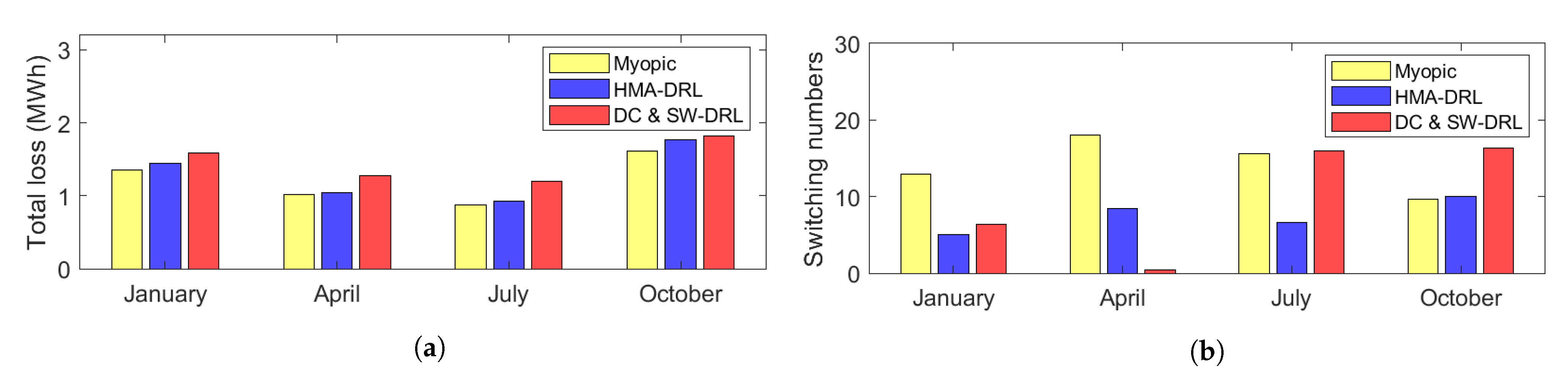
In this study, we propose a heterogeneous multi-agent deep reinforcement learning (HMA-DRL) algorithm to minimize network power loss while maintaining the voltage levels within the specified operational range. We considered two control entities: switches and solar PV smart inverters (PVSIs). Considering ownership of the two control entities, they are controlled by the DSO (centralized) and PV generation companies (distributed), respectively. In the proposed algorithm, the agent at the central control center operates switches, that is, the dynamic DNR, with complete information on the distribution system. It aims to minimize the power loss in the system while maintaining the voltage levels in the normal range. On the other hand, the agents at PVSIs take the action of reactive power output with local information. They do not require any information from neighbors or the DSO. The agents at PVSIs only aim to maintain their local voltage levels within the normal range. The heterogeneities of ownership, level of information acquisition, and actions make the proposed HMA-DRL algorithm practical for a real distribution system. Through case studies using the modified 33-bus distribution test feeder, the proposed HMA-DRL algorithm performs the best among model-free algorithms in terms of the total power loss in the distribution system. It shows a performance of 93.13% of Myopic, which can be regarded as the optimal solution. In addition, the proposed HMA-DRL algorithm shows stable and robust performance because it shows good performance throughout the year, and the standard deviation of its performance has the smallest value among the different schemes compared.
In future work, we plan to investigate a more robust approach using safe reinforcement learning (RL) to protect distribution networks from unexplainable actions [36]. Additionally, energy storage systems can be considered to further improve system performance.

Author Contributions

Methodology, S.-H.L.; Validation, S.-H.L.; Writing—original draft, S.-H.L.; Writing—review & editing, S.-G.Y.; Supervision, S.-G.Y. All authors have read and agreed to the published version of the manuscript.

Funding

This study is supported in part by the Ministry of Science, ICT (MSIT), Korea, under the High-Potential Individuals Global Training Program (2021-0-01525) supervised by the Institute for Information & Communications Technology Planning & Evaluation (IITP), and in part by the National Research Foundation of Korea (NRF) grant funded by the MSIT (No. 2020R1F1A1075137).

Data Availability Statement

Publicly available datasets were analyzed in this study. This data can be found here: (1) [https://www.data.go.kr/dataset/15025486/fileData.do], (2) [http://wzy.ece.iastate.edu/Testsystem.html].

Conflicts of Interest

The authors declare no conflict of interest.

Abbreviations

N n  Set and index of buses
K Kk  Set, the number, and index of buses installed PV
E e  Set and index of lines, respectively.
O o  Set and index of lines installed remote-controlled switches
T Tt  Set, the number, and index of period
ρ t   Efficiency of PV output
V t n   Phasor voltage in bus n at hour t
I t e   Phasor current in line e at hour t
P t n   Net real power in bus n at hour t
Q t n   Net reactive power in bus n at hour t
l t   Power loss at hour t in initial topology
l t D N R   Power loss at hour t after switches control
R e   Resistance of line e
G m n   Conductance between buses m and n
B m n   Susceptance between buses m and n
j t o   Switched status of line o
δ n   Phase angle in bus n
b t n m   Binary variable representing the parent–child relationship
N ¯ S W   Maximum number of switching number

References

  1. Tahir, M.; Nassar, M.E.; El-Shatshat, R.; Salama, M.M.A. A review of Volt/Var control techniques in passive and active power distribution networks. In Proceedings of the 2016 IEEE Smart Energy Grid Engineering (SEGE), Oshawa, ON, Canada, 21–24 August 2016; pp. 57–63. [Google Scholar] [CrossRef]
  2. Jabr, R.A.; Singh, R.; Pal, B.C. Minimum loss network reconfiguration using mixed-integer convex programming. IEEE Trans. Power Syst. 2012, 27, 1106–1115. [Google Scholar] [CrossRef]
  3. Dantas, F.V.; Fitiwi, D.Z.; Santos, S.F.; Catalao, J.P.S. Dynamic reconfiguration of distribution network systems: A key flexibility option for RES integration. In Proceedings of the 2017 IEEE International Conference on Environment and Electrical Engineering and 2017 IEEE Industrial and Commercial Power Systems Europe (EEEIC/I&CPS Europe), Milan, Italy, 6–9 June 2017; pp. 1–6. [Google Scholar] [CrossRef]
  4. Mosbah, M.; Arif, S.; Mohammedi, R.D.; Hellal, A. Optimum dynamic distribution network reconfiguration using minimum spanning tree algorithm. In Proceedings of the 2017 5th International Conference on Electrical Engineering-Boumerdes (ICEE-B), Boumerdes, Algeria, 29–31 October 2017; pp. 1–6. [Google Scholar] [CrossRef]
  5. Capitanescu, F.; Ochoa, L.F.; Margossian, H.; Hatziargyriou, N.D. Assessing the potential of network reconfiguration to improve distributed generation hosting capacity in active distribution systems. IEEE Trans. Power Syst. 2014, 30, 346–356. [Google Scholar] [CrossRef]
  6. Izadi, M.; Safdarian, A. Financial risk evaluation of RCS deployment in distribution systems. IEEE Syst. J. 2018, 13, 692–701. [Google Scholar] [CrossRef]
  7. Pamshetti, V.B.; Singh, S.; Singh, S.P. Combined impact of network reconfiguration and volt-var control devices on energy savings in the presence of distributed generation. IEEE Syst. J. 2019, 14, 995–1006. [Google Scholar] [CrossRef]
  8. Weckx, S.; Gonzalez, C.; Driesen, J. Combined central and local active and reactive power control of PV inverters. IEEE Trans. Sustain. Energy 2014, 5, 776–784. [Google Scholar] [CrossRef]
  9. Qiao, X.; Luo, Y.; Xiao, J.; Li, Y.; Jiang, L.; Shao, X.; Cao, Y. Optimal scheduling of distribution network incorporating topology reconfiguration, BES and load response: A MILP model. CSEE J. Power Energy Syst. 2020, 8, 743–756. [Google Scholar] [CrossRef]
  10. Sheng, W.; Liu, K.Y.; Cheng, S.; Meng, X.; Dai, W. A trust region SQP method for coordinated voltage control in smart distribution grid. IEEE Trans. Smart Grid 2018, 7, 381–391. [Google Scholar] [CrossRef]
  11. Ji, H.; Wang, C.; Li, P.; Zhao, J.; Song, G.; Ding, F.; Wu, J. A centralized-based method to determine the local voltage control strategies of distributed generator operation in active distribution networks. Appl. Energy 2018, 228, 2024–2036. [Google Scholar] [CrossRef]
  12. Yang, Q.; Wang, G.; Sadeghi, A.; Giannakis, G.B.; Sun, J. Two-timescale voltage control in distribution grids using deep reinforcement learning. IEEE Trans. Smart Grid 2019, 11, 2313–2323. [Google Scholar] [CrossRef] [Green Version]
  13. Gao, Y.; Shi, J.; Wang, W.; Yu, N. Dynamic distribution network reconfiguration using reinforcement learning. In Proceedings of the 2019 IEEE International Conference on Communications, Control, and Computing Technologies for Smart Grids (SmartGridComm), Beijing, China, 21–23 October 2019; pp. 1–7. [Google Scholar] [CrossRef]
  14. Gao, Y.; Wang, W.; Shi, J.; Yu, N. Batch-constrained reinforcement learning for dynamic distribution network reconfiguration. IEEE Trans. Smart Grid 2020, 11, 5357–5369. [Google Scholar] [CrossRef]
  15. Li, C.; Jin, C.; Sharma, R. Coordination of PV smart inverters using deep reinforcement learning for grid voltage regulation. In Proceedings of the 2019 18th IEEE International Conference On Machine Learning And Applications (ICMLA), Boca Raton, FL, USA, 16–19 December 2019; pp. 1930–1937. [Google Scholar] [CrossRef] [Green Version]
  16. Liu, H.; Wu, W. Two-stage deep reinforcement learning for inverter-based volt-var control in active distribution networks. IEEE Trans. Smart Grid 2020, 12, 2037–2047. [Google Scholar] [CrossRef]
  17. Cao, D.; Hu, W.; Zhao, J.; Huang, Q.; Chen, Z.; Blaabjerg, F. A multi-agent deep reinforcement learning based voltage regulation using coordinated PV inverters. IEEE Trans. Power Syst. 2020, 35, 4120–4123. [Google Scholar] [CrossRef]
  18. Lim, S.H.; Nishimwe, L.F.H.; Yoon, S.G. DQN Based Dynamic Distribution Network Reconfiguration for Energy Loss Minimization Considering DGs. In Proceedings of the CIRED 2021—The 26th International Conference and Exhibition on Electricity Distribution, online, 20–23 September 2021; pp. 20–23. [Google Scholar] [CrossRef]
  19. Zhang, Y.; Wang, X.; Wang, J.; Zhang, Y. Deep reinforcement learning based volt-var optimization in smart distribution systems. IEEE Trans. Smart Grid 2020, 12, 361–371. [Google Scholar] [CrossRef]
  20. Gao, Y.; Wang, W.; Yu, N. Consensus multi-agent reinforcement learning for volt-var control in power distribution networks. IEEE Trans. Smart Grid 2021, 12, 3594–3604. [Google Scholar] [CrossRef]
  21. Sun, X.; Qiu, J. Two-stage volt/var control in active distribution networks with multi-agent deep reinforcement learning method. IEEE Trans. Smart Grid 2021, 12, 2903–2912. [Google Scholar] [CrossRef]
  22. Seuss, J.; Reno, M.J.; Broderick, R.J.; Grijalva, S. Improving distribution network PV hosting capacity via smart inverter reactive power support. In Proceedings of the 2015 IEEE Power and Energy Society General Meeting, Denver, CO, USA, 26–30 July 2015; pp. 1–5. [Google Scholar] [CrossRef]
  23. Pourjafari, E.; Reformat, M. A support vector regression based model predictive control for volt-var optimization of distribution systems. IEEE Access 2019, 7, 93352–93363. [Google Scholar] [CrossRef]
  24. Liu, Q.; Guo, Y.; Deng, L.; Tang, W.; Sun, H.; Huang, W. Robust Offline Deep Reinforcement Learning for Volt-Var Control in Active Distribution Networks. In Proceedings of the 2021 IEEE 5th Conference on Energy Internet and Energy System Integration (EI2), Taiyuan, China, 22–24 October 2021; pp. 442–448. [Google Scholar] [CrossRef]
  25. Nguyen, T.T.; Nguyen, N.D.; Nahavandi, S. Deep reinforcement learning for multiagent systems: A review of challenges, solutions, and applications. IEEE Trans. Cybern. 2020, 50, 3826–3839. [Google Scholar] [CrossRef] [Green Version]
  26. Tampuu, A.; Matiisen, T.; Kodelja, D.; Kuzovkin, I.; Korjus, K.; Aru, J.; Aru, J.; Vicente, R. Multiagent cooperation and competition with deep reinforcement learning. PloS ONE 2017, 12, e0172395. [Google Scholar] [CrossRef] [Green Version]
  27. Kuzlu, M.; Pipattanasomporn, M.; Rahman, S. Communication network requirements for major smart grid applications in HAN, NAN and WAN. Comput. Netw. 2014, 67, 74–88. [Google Scholar] [CrossRef]
  28. Korea Western Power Company Limited. Photovoltaic Generation Status of Korea Western Power Company Limited. Available online: https://www.data.go.kr/dataset/15025486/fileData.do (accessed on 30 October 2022).
  29. Lee, H.J.; Yoon, K.H.; Shin, J.W.; Kim, J.C.; Cho, S.M. Optimal parameters of volt–var function in smart inverters for improving system performance. Energies 2020, 13, 2294. [Google Scholar] [CrossRef]
  30. Mnih, V.; Kavukcuoglu, K.; Silver, D.; Graves, A.; Antonoglou, I.; Wierstra, D.; Riedmiller, M. Playing atari with deep reinforcement learning. arXiv, 2013; arXiv:1312.5602. [Google Scholar]
  31. Mishra, S.; Das, D.; Paul, S. A comprehensive review on power distribution network reconfiguration. Energy Syst. 2017, 8, 227–284. [Google Scholar] [CrossRef]
  32. Korea Electric Power Company (KEPCO). Regulation on the Use of Electrical Equipment for Transmission Distribution System. Available online: http://cyber.kepco.co.kr/ckepco/front/jsp/CY/H/C/CYHCHP00704.jsp (accessed on 30 October 2022).
  33. Wang, Z., Dr. Zhaoyu Wang’s Homepage. Available online: http://wzy.ece.iastate.edu/Testsystem.html (accessed on 30 October 2022).
  34. Lei, S.; Hou, Y.; Qiu, F.; Yan, J. Identification of critical switches for integrating renewable distributed generation by dynamic network reconfiguration. IEEE Trans. Sustain. Energy 2017, 9, 420–432. [Google Scholar] [CrossRef]
  35. Thurner, L.; Scheidler, A.; Schäfer, F.; Menke, J.H.; Dollichon, J.; Meier, F.; Braun, M. Pandapower—An Open-Source Python Tool for Convenient Modeling, Analysis and Optimization of Electric Power Systems. IEEE Trans. Power Syst. 2018, 33, 6510–6521. [Google Scholar] [CrossRef] [Green Version]
  36. Kou, P.; Liang, D.; Wang, C.; Wu, Z.; Gao, L. Safe deep reinforcement learning-based constrained optimal control scheme for active distribution networks. Appl. Energy 2020, 264, 114772. [Google Scholar] [CrossRef]
Figure 1. System model.
Energies 15 09220 g001
Figure 2. A framework of the proposed HMA-DRL algorithm.
Energies 15 09220 g002
Figure 3. Modified 33-bus distribution test feeder. There are two solar PV generators at buses 18 and 33; five sectionalizing switches (7), (14), (17), (24), and (28); and five tie switches (33), (34), (35), (36), and (37).
Energies 15 09220 g003
Figure 4. Cumulative reward during the training procedure of HMA-DRL in January.
Energies 15 09220 g004
Figure 5. Daily average performance comparison using seasonal data. (a) Total loss for test days; (b) Switching numbers for test days.
Energies 15 09220 g005
Figure 6. Voltage profile for six test days in January. (a) Voltage profile without control (Baseline); (b) voltage profile with the proposed HMA-DRL algorithm.
Energies 15 09220 g006
Figure 7. The action of agent at PVSI and CCC on the first day. (a) Reactive power of smart inverter at bus 18; (b) comparison of network power loss; (c) voltage profile comparison 1 at bus 18; (d) voltage profile comparison 2 at bus 18 (DRL-based algorithms).
Energies 15 09220 g007
Figure 8. Distribution system topology of the test day. (a) Topology index for three algorithms (DC and SW-DRL, Myopic, and HMA-DRL); (b) topology 52.
Energies 15 09220 g008aEnergies 15 09220 g008b
Table 1. Line parameters of the distribution system.
CNCV-W325ACSR/AWOC-160ACSR/AWOC-095
R ( Ω /km)0.0750.1820.304
X ( Ω /km)0.1250.3910.441
Table 2. DQN hyperparameters.
Agent at PVSIAgent at CCC
N e p 1600
T600 h (25 days)
Batch size for updating DQN128
Replay buffer size50,000
γ 00.85
β 0.01-
w s w -3
w p v 0.5-
Size of neural network{4, 300, 300, 41}{46, 700, 700, 63}
Table 3. Daily average performance comparison in terms of voltage violation, loss, and the number of switching. (HMA-DRL: the proposed heterogeneous multi-agent DRL; PV-DRL: DRL for PVSIs; SW-DRL: DRL for switches; DC: droop control.
MethodCurtailed Energy (MWh)Network Loss (MWh)Total Loss (MWh)Switching Numbers
Baseline-1.611.61-
Curtailment9.040.959.99-
Myopic01.221.2213.91
HMA-DRL0.041.271.317.48
PV-DRL0.081.671.75-
SW-DRL7.671.439.0911.30
DC01.911.91-
DC & SW-DRL01.471.4710.17
Table 4. Frequency and severity of the overvoltage problems during the test period.
Method N over V avg (p.u.) V std (p.u.) V max (p.u.)
Baseline6981.04850.00631.0720
HMA-DRL31.04150.00071.0425
PV-DRL71.04270.00121.0449
SW-DRL4701.05170.01031.0906
Publisher’s Note: MDPI stays neutral with regard to jurisdictional claims in published maps and institutional affiliations.

