Towards Optimization of Energy Consumption of Tello Quad-Rotor with Mpc Model Implementation

Abstract

For the last decade, there has been great interest in studying dynamic control for unmanned aerial vehicles, but drones—although a useful technology in different areas—are prone to several issues, such as instability, the high energy consumption of batteries, and the inaccuracy of tracking targets. Different approaches have been proposed for dealing with nonlinearity issues, which represent the most important features of this system. This paper focuses on the most common control strategy, known as model predictive control (MPC), with its two branches, linear (LMPC) and nonlinear (NLMPC). The aim is to develop a model based on sensors embedded in a Tello quad-rotor used for indoor purposes. The original controller of the Tello quad-rotor is supposed to be the slave, and the designed model predictive controller was created in MATLAB. The design was imported to another embedded system, considered the master. The objective of this model is to track the reference trajectory while maintaining the stability of the system and ensuring low energy consumption. The case study in this paper compares linear and nonlinear model predictive control (MPC). The results show the efficiency of NLMPC, which provides more promising results compared to LMPC. The comparison concentrates on the energy consumption, the tracked trajectory, and the execution time. The main finding of this research is that NLMPC is a good solution to smoothly track the reference trajectory. The controller in this case processes faster, but the rotors consume more energy because of the increased values of control inputs calculated by the nonlinear controller.

1. Introduction

Drones, abbreviated as UAVs (unmanned aerial vehicles), are unmanned aircraft capable of carrying out a mission autonomously by being self-piloted or semi-autonomous using remote control [1,2]. The primary function of these vehicles is to extend human vision beyond the natural horizon to accomplish work in risky or hostile environments. The military has implemented the first applications of drones for surveillance or reconnaissance missions without the risk of human losses. More recently, civil applications have appeared, such as the prevention of forest fires, the inspection of engineering structures, the energy flow monitoring of motorway traffic, or the collection of meteorological data. However, the use of civilian drones remains limited because non-military drones still need to be fully integrated into civil airspace [2,3].

The classification of existing UAVs differs depending on the country and its army [4]. UAVs can be classified according to their size, endurance, flight altitude, function, mass, payload, etc. The most accepted classification divides UAVs according to their size and endurance, where, generally, five categories of UAVs exist, from aircraft UAVs with a wingspan of about 30 m to flapping wings a few millimeters long.

In this paper, the focus is on quad-rotor UAVs, known as drones with multiple rotors. Multi-rotor UAVs are certainly the best-known and most widespread aeromechanic configurations among autonomous aerial vehicles [5]. These aircraft are usually equipped with four rotors, but there are also some with six or even eight rotors. The mechanical simplicity of this type of vehicle makes it a widely used configuration for the realization of experimental platforms at reduced costs [6]. The operation of multi-rotor drones is quite particular, where a plus or cross configuration can be used [7]. First, to compensate for the torque reaction, the rotation of the rotors’ direction is reversed two by two. In addition, the translation and the rotation movements according to the three axes are carried out carefully by manipulating the rotational speeds of the different rotors. In fact, it is the difference in the lift that determines the inclination of the aircraft around the roll and pitch angles, allowing translational flight. Figure 1 shows the movement states of a quad-rotor with the cross configuration regarding the X-, Y-, and Z-axes [8].

Due to the very good distribution of lift in the horizontal plane, multi-rotor UAVs are particularly suitable for hovering and low-speed flights. On the other hand, this configuration is not recommended for high-speed translational flights nor for use in windy conditions. Moreover, this rotor configuration is restricted to small-sized aircraft because the size of the rotors increases with the increase in the mass of the drone.

The main goal in drone design is to achieve a high degree of autonomy to make decisions and remain in a stable state. This can be achieved based on the embedded systems in the body, which are the measurement system and the controller. The measurement system in the drone is responsible for the collection of information on the state of the drone and its environment, and three types of sensors can be found [9,10]:

• Sensors for measuring attitude, such as gyroscopes to measure angular position and angular velocity, accelerometers to measure acceleration, and magnetometers to measure the direction of the magnetic field and scan the area and detect metals in space;
• Sensors for measuring the velocity and position of the drone, such as an altimeter, GPS, and camera;
• Sensors for detecting obstacles around the drone, such as ultrasonic sensors and telemeter lasers.

The information obtained from the measurement system is transferred to the control part as digital signals, where the data are processed by the control system. The control system based on a mathematical algorithm generates control signals that allow the drone to move in an appropriate way. This is based on a mathematical representation of the drone’s mechanical body and on the measurement signals from the on-board sensors. Its role is, above all, to guarantee the stability of the device during the autonomous flight phase. Despite a general principle that is relatively simple to understand, the design of such a system is rather complex and requires special attention. Indeed, UAVs, and more particularly rotary-wing UAVs such as quad-rotors, are under-actuated systems and sensitive to aerodynamic disturbances, whose dynamics are highly nonlinear [11,12]. Moreover, this presents significant coupling between the system’s state variables and its control inputs. The coupling characterizes the fact that any change in a control input affects not only the variable of interest but also the others [13].

Based on Newton–Euler equations or the energetic Lagrange derivative, many scientists have suggested approaches to designing dynamic models of drones, beginning with the mathematical model for the kinematic and dynamic models [13,14,15] for considering the behavior of the quad-rotor in different flight conditions (stationary, in translation, or in rotation). However, the main problem with these dynamic models is the difficulty of designing a “simple” control algorithm due to the complexity of the model, which is nonlinear. The first mission of the quad-rotor is to track a position from one point to another point in a 3D environment with respect to the given orientation. Under all of the previously cited challenging criteria, this task makes the object deal with the study of control theory by developing controllers that can succeed in tracking the trajectory and avoiding obstacles, all while optimizing the battery life of the drone.

The control strategy for the quad-rotor scope represents a major issue in this research field, where many scientists have suggested different implementations, including linear control strategies, such as PID, LQ, H infinity, and linear MPC, and nonlinear control approaches, such as backstepping control or sliding mode control and nonlinear MPC [16,17,18,19,20,21].

At the energy profile level, one of the biggest drawbacks of the quad-rotor is its battery life, meaning that the average mission does not exceed 15 min [22,23]. This is because existing controllers are typically designed to maximize the performance of tracking while providing a sufficient margin of stability. However, extracting the maximum performance results in greater consumption and, therefore, a reduction in the battery life. For this reason, several researchers have focused on regulation using the linear quadratic controller since it minimizes energy consumption. In addition, several strategies can improve fuel efficiency. Some examples can be cited:

• Minimization of errors: indeed, this is the classic approach; the fewer the errors committed in the pursuit of the desired trajectory, the less energy spent [24];
• Fuzzy logic applied to altitude control: climbing or descending consumes double or even more energy because this movement causes the rotation of the four engines simultaneously, so one possibility is establishing fuzzy logic between the flight height and the battery state of charge [25];
• The search for an optimal trajectory: energy consumption can be reduced by using or avoiding air currents and thus by finding the flight path that is least costly in terms of energy compared to a direct flight to the destination [25].

The motivation for this research is related to building a powerful customized embedded controller for the Tello EDU drone using the Xilinx Kria board in the future [26]. To achieve the main goal, this research started with the linear and nonlinear model predictive control design. It is assumed that the Kria board will handle the designed controller in order to command Tello EDU to execute indoor movements, all while maintaining stability and optimizing the energy consumption of the rotors. The quad-rotor already has a basic embedded system that fulfills simple commands for take-off and landing motions, with low accuracy and stability.

This work introduces a completely new model design for linear and nonlinear MPC controllers intended to be used for indoor applications with the Tello drone. Compared to previous works [27,28,29,30], this paper also provides a methodology for designing MPC controllers considering the real system parameters, the limitations of linear MPC, and approaches in order to increase the energy efficiency.

This paper includes the following parts: First, the process to identify the dynamic mathematical model of the Tello drone with the actual parameters is presented. This model is purely nonlinear due to the strong coupling between the state variables and the control inputs, but in addition, its dynamics are under-actuated, i.e., the amount of information, which is four times less than the number of outputs, which is six (the degrees of freedom). In the second part, after creating the dynamic model, the methodology to build a control strategy is shown. Two approaches are taken into consideration in this research: the first assumes that the system is linear, so model predictive control is applied. This approach requires linearizing the dynamic model around an equilibrium point, called the hover position. The second approach assumes that the system is dealing with reality and is nonlinear. Therefore, nonlinear model predictive control is applied to track the reference trajectory. A detailed comparison will be presented regarding the motion tracking, stability, and energy profile. This paper shows how the inputs influence the effect of predictive model control on energy consumption. The input variables for the drone represent the angular velocities of the four rotors. In the third section, the simulation results are discussed, and a comparison is made to understand the potential of using a nonlinear controller instead of a linear one. Finally, conclusions and further work are presented.

2. Materials and Methods

The main aim of this work was to build a customized embedded system for the Tello EDU quad-rotor. The customized embedded system is based on a System on Chip (SOC) from AMD Xilinx and implements a control strategy based on MPC. Figure 2 presents the plan for the main target. To start the process, the research began by developing suitable model predictive control for the Tello EDU quad-rotor. This type of drone is helpful for education and research purposes. The control model is based on the dynamic mathematical model of the drone and its fundamental parameters; therefore, this paper presents a methodology for building a suitable control strategy based on the following points:

• The conditions are taken into consideration to identify the dynamic mathematical model;
• The parameters of the Tello EDU quad-rotor are identified;
• Linear and nonlinear model predictive control is used;
• An in-depth comparison is made to show the effectiveness of a nonlinear controller and how the optimization of energy consumption can be achieved for the control part.

Figure 2. The plan for building the customized embedded system for Tello Edu.

Figure 2. The plan for building the customized embedded system for Tello Edu.

The simulation was performed using MATLAB Simulink, which offers different functions that can help to efficiently achieve the research target, especially since setting parameters and analyzing the results in Simulink are more user-friendly than using MATLAB Script.

In the following, the paper will highlight the methods used to build the optimal controller, starting by modeling the dynamics of the Tello quad-rotor and then dealing with the control strategy by getting familiar with a model predictive controller in general and demonstrating how to successfully tune both control types (linear and nonlinear).

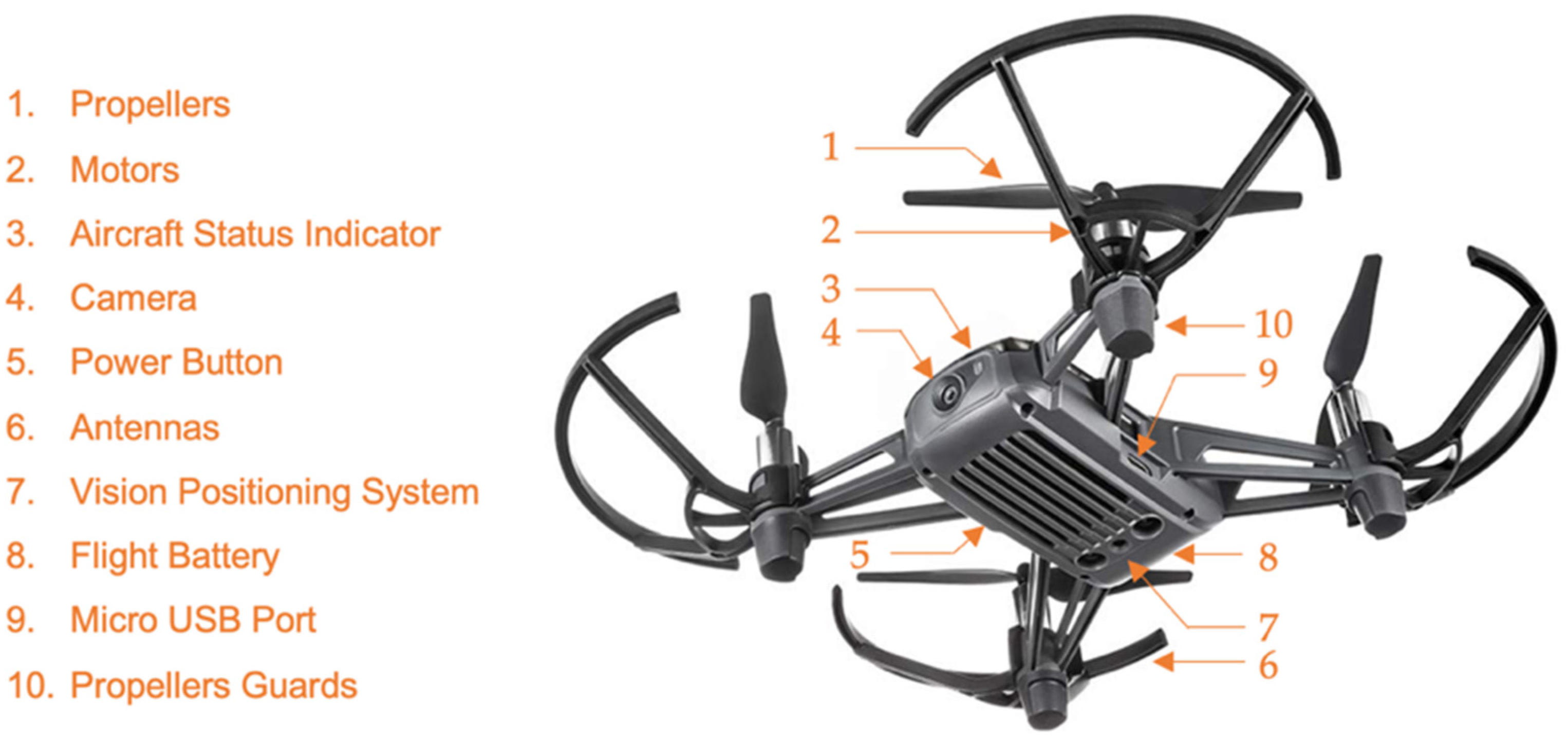
2.1. Tello Quad-Rotor Model

The Tello EDU quad-rotor model [26] is an impressive and programmable drone that is valuable for educational purposes. The system is dedicated to students who are learning programming languages such as Scratch, Python, and Swift and for developing AI functions such as a fly-in swarm, upgrading with SDK 2.0, embedding with DJI’s flight control technology, and supporting electronic image stabilization.

Figure 3 presents the Tello quad-rotor with its specifications. The drone features a vision positioning system and an on-board camera based on an advanced flight controller to hover in a precise place, as is suitable for flying indoors; its maximum flight time is around 13 min, and the maximum flight distance is 100 m. These specifications are critical in showing the advantages and drawbacks that they have. For example, when the drone flies indoors, this characteristic will neglect the wind and gyroscopic effects as a disturbance in the system. Additionally, it is a motivation to optimize the energy profile of this drone to lengthen the flight time by using optimal control strategies.

The objective was to develop a new predictive control model for the Tello drone using its basic sensors, identified as a complete system: the vision positioning system helps the aircraft to maintain its current position, and its main components are the camera and the 3D infrared module located on the underside of the plane.

2.2. Quad-Rotor Mathematical Model

Designing a suitable controller for an appropriate drone requires first modeling the mathematical dynamics of the plant.

This helps to explain how the drone moves and what forces and torques are applied. How many motions there are? Which velocities are needed to execute different flight modes? Therefore, one can identify the inputs, outputs, state variables, and disturbances in the central system.

Figure 4 describes the dynamic structure of the Tello drone in the body and inertial frames, where the corresponding angular velocities, torques, and forces created by the four rotors (numbered from 1 to 4) are presented. The drone’s movement is generated by differential thrust forces between F2 and F4 that generate rotation around the X-axis, known as roll motion. On the other hand, differential thrust forces between F1 and F3 will generate rotation around the Y-axis, known as pitch motion. In contrast, rotation around the Z-axis, the yaw motion, is caused by differential torques between clockwise and anticlockwise rotors, i.e., $\left({\tau }_1-{\tau }_2+{\tau }_3-{\tau }_4\right)$.

The modeling of UAVs is a delicate task since the system’s dynamics are strongly nonlinear and fully coupled. Many reviews have explained the methodology for modeling such systems. This paper presents the exact strategy to obtain both linear and nonlinear dynamic models based on the Tello drone’s main parameters. The calculation of the mathematical model is based on some simplifications; here are the different working hypotheses [31]:

• The structure of the quad-rotor is assumed to be rigid and symmetrical, which means that the matrix of inertia is assumed to be diagonal;
• The propellers are assumed to be rigid in order to be able to neglect the effect of their deformation during rotation;
• The center of mass and the origin of the frame linked to the structure coincide;
• The lift and drag forces are proportional to the square of the rotors’ rotation speed, which is a very close approximation of the aerodynamic behavior;
• To evaluate the quad-rotor’s mathematical model, two frames were used: a fixed inertial frame to the Earth ${\mathrm{R}}_{\mathrm{f}}$ and a second mobile frame fixed in the quad-rotor ${\mathrm{R}}_{\mathrm{m}}$. The transformation matrix gives the passage between the body frame and the inertial frame$\mathrm{T}$, which contains the orientation and the mobile position reference relative to the fixed reference.

Figure 4 shows the axis convention taken for the Tello drone to model the mathematical dynamics, where the forces, inertial moments, and angular velocities are described.

The quad-rotor system is a light structural flight vehicle. Therefore, the gyroscopic effects resulting from the rotation of the rigid body and the four propellers should be included in the dynamic model. However, the dynamic model of the system is obtained under the assumption that the vehicle is a rigid body in the spatial domain with different forces and torques. The mathematical model presented here is based on Newton and Euler equations for 3D rigid-body motion [31].

Let ${\left[\mathrm{x} \mathrm{y} \mathrm{z} \varphi \mathsf{\theta } \mathsf{\psi }\right]}^{\mathrm{T}}$ denote the vector containing the linear and angular positions of the quad-rotor in the inertial frame ${\mathrm{F}}_{\mathrm{i}}$, and let ${\left[\mathrm{u} \mathrm{v} \mathrm{w} \mathrm{p} \mathrm{q} \mathrm{r}\right]}^{\mathrm{T}}$ denote the vector containing the linear and angular velocities in the body frame F_b. From 3D body dynamics, it follows that the two reference frames are linked by the following relations:

$$v=\left[\begin{array}{c}{v}_x^i\\ v_y^i\\ v_z^i\end{array}\right]=\left[\begin{array}{c}\dot{x}\\ \dot{y}\\ \dot{z}\end{array}\right]=R·v_b=R·\left[\begin{array}{c}u\\ v\\ w\end{array}\right]$$

(1)

$$\mathsf{\Omega }=\left[\begin{array}{c}{\mathsf{\Omega }}_x^b\\ {\mathsf{\Omega }}_y^b\\ {\mathsf{\Omega }}_z^b\end{array}\right]=\left[\begin{array}{c}p\\ q\\ r\end{array}\right]=T·\left[\begin{array}{c}\dot{\varphi }\\ \dot{\theta }\\ \dot{\psi }\end{array}\right]$$

(2)

where $\mathrm{v}$ is the linear velocity, $\mathsf{\Omega }$ is the rotation velocity, R is the rotation matrix describing the rotation from the body reference system to the inertial reference, and T is the matrix for angular transformation, where to obtain ${[\dot{\mathsf{\varphi }} \dot{\mathsf{\theta }} \dot{\mathsf{\psi }}]}^{\mathrm{T}}$, the inverse of matrix T is needed.

$$R=R_b^i=\left[\begin{array}{ccc}C\psi C\theta & C\psi S\psi S\theta -C\varphi S\psi & C\varphi S\theta C\psi +S\varphi S\psi \\ C\theta S\psi & S\varphi S\theta S\psi +C\varphi C\psi & C\varphi S\theta S\psi -S\varphi C\psi \\ -S\theta & S\varphi C\theta & C\varphi C\theta \end{array}\right]$$

(3)

$$T=\left[\begin{array}{ccc}1& 0& -S\theta \\ 0& C\varphi & C\theta S\varphi \\ 0& -S\varphi & C\varphi C\theta \end{array}\right], T^{-1}=\left[\begin{array}{ccc}1& S\theta T\theta & C\varphi T\theta \\ 0& C\theta & -S\theta \\ 0& \frac{S\varphi }{C\theta }& \frac{C\varphi }{C\theta }\end{array}\right]$$

(4)

where $C\theta$,$S\varphi$, and $\mathrm{T}\varphi$ represent cosine, sine, and tangent. From the two relations, the kinematic model for the quad-rotor is obtained as follows:

$$\{\begin{array}{c}\begin{array}{c}\dot{x}=u\left[C\psi C\theta \right]+v\left[C\psi S\psi S\theta -C\varphi S\psi \right]+w\left[C\varphi S\theta C\psi +S\varphi S\psi \right]\\ \dot{y}=u\left[C\theta S\psi \right]+v\left[S\varphi S\theta S\psi +C\varphi C\psi \right]+w\left[C\varphi S\theta S\psi -S\varphi C\psi \right]\\ \dot{z}=u\left[-S\theta \right]+v\left[S\varphi C\theta \right]+w\left[C\varphi C\theta \right]\end{array}\\ \begin{array}{c}\dot{\varphi }=p+q\left[S\varphi T\theta \right]+r\left[C\varphi T\theta \right] \\ \dot{\theta }=q\left[C\varphi \right]+r\left[-S\varphi \right]\\ \dot{\psi }=q\left[\frac{S\varphi }{C\theta }\right]+r\left[\frac{C\varphi }{C\theta }\right]\end{array}\end{array}$$

(5)

The vector $\left[\mathrm{u} \mathrm{v} \mathrm{w} \mathrm{p} \mathrm{q} \mathrm{r}\right]{ }^{\mathrm{T}}$ is obtained using an IMU system with the data obtained from the accelerometer and gyroscope sensors. In order to obtain the dynamic model and list all of the physical effects, forces, and inertia moments exerted on the system, the following factors are considered.

• The weight force of the quad-rotor is given by:

$$P=m·g$$

(6)

where m is the total mass of the rigid body, and g is the gravity.

• The thrust forces created by the four rotors are perpendicular to the plane of the propellers and are proportional to the square of the rotational speed of the motors. The thrust forces are given by:

$$F_i=b·{\omega }_i^2$$

(7)

where $\mathrm{i}=1\dots 4$; $\mathrm{b}$ is the coefficient of lift and depends on the shape and number of blades and the air density; $\mathsf{\omega }$ is the angular velocity of the engine.

• The drag force is the coupling between the pressure force and the viscous frictional force.

In this case, two drag forces are acting on the system: the drag in the propellers and the drag along the axes (x, y, z).

The drag in the propellers acts on the blades; it is proportional to the density of the air, to the shape of the edges, and to the square of the rotation velocity of the propeller and is given by the following relation:

$$F_{da}=d·{\omega }^2$$

(8)

where d is the drag coefficient, which depends on the manufacture of the propeller.

The drag along the axes (x, y, z) is due to the movement of the body of the quad-rotor:

$$F_{dl}=K_{ft}·v$$

(9)

where ${\mathrm{K}}_{\mathrm{ft}}$ is the translational drag coefficient, and v is the linear velocity.

Regarding the inertial moments applied to the system, the following variables are considered.

• The inertial moments due to the thrust force: The rotation around the X- and Y-axes is due to the inertial moment created by the difference between the thrust forces of Rotors 2 and 4 and 1 and 3, respectively:

$$\{\begin{array}{c}{M}_x=l\left(F_4-F_2\right)=lb\left({\omega }_4^2-{\omega }_2^2\right)\\ M_y=l\left(F_3-F_1\right)=lb\left({\omega }_3^2-{\omega }_1^2\right)\end{array}$$

(10)

where l is the length of the arm between the rotor and the center of gravity of the quad-rotor.

• The inertial moment due to drag forces: The rotation around the z-axis is due to the reactive torque caused by the drag torques in each propeller:

$$M_z=d\left({\omega }_1^2-{\omega }_2^2+{\omega }_3^2-{\omega }_4^2\right)$$

(11)

• The inertial moment resulting from aerodynamic friction is given by:

$$M_a=K_{fa}·{\mathsf{\Omega }}^2$$

(12)

where $K_{fa}$ the coefficient of aerodynamic friction angular velocity.

• Gyroscopic effect: This effect is defined as the difficulty of modifying the position or the orientation of the plane of rotation of a rotating mass. In this case, there are two gyroscopic moments. The gyroscopic moment of the helices is given by the expression:

$$M_{gh}={\displaystyle \sum }_{i=1}^4\mathsf{\Omega }\wedge J_r{\left[\begin{array}{ccc}0& 0& {\left(-1\right)}^{i+1}·{\omega }_i\end{array}\right]}^T$$

(13)

The gyroscopic moment due to the movements of the quad-rotor is written:

$$M_{gm}=\Omega \wedge J\Omega$$

(14)

where ${\mathrm{J}}_{\mathrm{r}}$ in Equation (13) is the moment of inertia of the rotor, and J is the moment of inertia of the system.

Other aerodynamic effects (blade flapping effect, air friction, and ground effects) that can disturb the movement of the quad-rotor are not taken into consideration in this article, as their effects at low speed can be neglected.

By using Newton–Euler equations, the dynamics of a rigid body under external forces and moments in the body frame can be formulated as follows:

• Dynamic equation of translation motion

$$m{ \dot{\mathrm{v}}}_{inertial}={\displaystyle \sum }{F}_{external}$$

(15)

where m is the mass of the rigid body, and ${\mathrm{v}}_{inertial}$ and $F_{external}$ are the linear velocity and the forces projected in the inertial frame, respectively. Using the rotation matrix to transform forces from the rigid body frame to the inertial body frame, the equations are:

$$m\ddot{\xi }=F_t+F_{dl}+F_g$$

(16)

$$F_t=R{\left[\begin{array}{ccc}0& 0& {\displaystyle \sum }_{i=1}^4{F}_i\end{array}\right]}^T; F_g={\left[\begin{array}{ccc}0& 0& -mg\end{array}\right]}^T$$

(17)

$$F_{dl}=\left[\begin{array}{ccc}-K_{ftx}& 0& 0\\ 0& -K_{fty}& 0\\ 0& 0& -K_{ftz}\end{array}\right]\dot{\xi } ; \mathrm{where} \xi =\left[\begin{array}{c}x\\ y\\ z\end{array}\right]$$

(18)

After replacing all of the terms presented before, the results are:

$$m\left[\begin{array}{c}\ddot{x}\\ \ddot{y}\\ \ddot{z}\end{array}\right]=\left[\begin{array}{c}C\varphi S\theta C\psi +S\varphi S\psi \\ C\varphi S\theta S\psi -S\varphi C\psi \\ C\varphi C\theta \end{array}\right]{\displaystyle \sum }_{i=1}^4{F}_i-\left[\begin{array}{c}{K}_{ftx}\dot{x}\\ K_{ftx}\dot{y}\\ K_{ftx}\dot{z}\end{array}\right]-\left[\begin{array}{c}0\\ 0\\ mg\end{array}\right]$$

(19)

$$\{\begin{array}{c}\ddot{x}=\frac{1}{m}\left(C\varphi S\theta C\psi +S\varphi S\psi \right)\left({\displaystyle {\displaystyle \sum }_{i=1}^4}{F}_i\right)-\frac{K_{ftx}}{m}\dot{x}\\ \ddot{y}=\frac{1}{m}\left(C\varphi S\theta S\psi -S\varphi C\psi \right)\left({\displaystyle {\displaystyle \sum }_{i=1}^4}{F}_i\right)-\frac{K_{fty}}{m}\dot{y}\\ \ddot{z}=\frac{1}{m}\left(C\varphi C\theta \right)\left({\displaystyle {\displaystyle \sum }_{i=1}^4}{F}_i\right)-\frac{K_{ftz}}{m}\dot{z}-g\end{array}$$

(20)

• Dynamic equation of rotation motion

Applying Euler’s rotation equation, the following equation is obtained:

$$J\dot{\Omega }+\Omega \times J\Omega ={\displaystyle \sum }{M}_{external}$$

(21)

where$\mathsf{\Omega }$ in this equation represents the rotation velocity present in the inertial axes, and $\mathrm{J}$ is the inertial tensor of the symmetric rigid body around its center of mass. ${\mathrm{M}}_{\mathrm{external}}$ represents the sum of moments acting on the vehicle:

$$J=\left[\begin{array}{ccc}{J}_{xx}& 0& 0\\ 0& J_{yy}& 0\\ 0& 0& J_{zz}\end{array}\right]$$

(22)

where ${\mathrm{J}}_{\mathrm{xx}}$, ${\mathrm{J}}_{\mathrm{yy}}$ and ${\mathrm{J}}_{\mathrm{zz}}$ are calculated according to the mass distribution by replacing the previous inertial moments:

$$J\dot{\Omega }=-\Omega \times J\Omega -M_a-M_{gh}+M_f$$

(23)

$$\mathrm{where}: M_f=\left[\begin{array}{c}{M}_x=lb\left({\omega }_4^2-{\omega }_2^2\right)\\ M_y=lb\left({\omega }_3^2-{\omega }_1^2\right)\\ M_z=d\left({\omega }_1^2-{\omega }_2^2+{\omega }_3^2-{\omega }_4^2\right)\end{array}\right]; M_a=\left[\begin{array}{c}{K}_{fax}{\dot{\varphi }}^2\\ K_{fay}{\dot{\theta }}^2\\ K_{faz}{\dot{\psi }}^2\end{array}\right]$$

(24)

After replacing all the terms in the equation, the equation results are:

$$\left[\begin{array}{ccc}{J}_{xx}& 0& 0\\ 0& J_{yy}& 0\\ 0& 0& J_{zz}\end{array}\right]\left[\begin{array}{c}\ddot{\varphi }\\ \ddot{\theta }\\ \ddot{\psi }\end{array}\right]=-\left[\begin{array}{c}\dot{\varphi }\\ \dot{\theta }\\ \dot{\psi }\end{array}\right]\wedge \left(\left[\begin{array}{ccc}{J}_{xx}& 0& 0\\ 0& J_{yy}& 0\\ 0& 0& J_{zz}\end{array}\right]\left[\begin{array}{c}\dot{\varphi }\\ \dot{\theta }\\ \dot{\psi }\end{array}\right]\right)-\left[\begin{array}{c}-J_r{\overline{\mathsf{\Omega }}}_r\dot{\dot{\theta }}\\ J_r{\overline{\mathsf{\Omega }}}_r\dot{\varphi }\\ 0\end{array}\right]-\left[\begin{array}{c}{K}_{fax}{\dot{\varphi }}^2\\ K_{fay}{\dot{\theta }}^2\\ K_{faz}{\dot{\psi }}^2\end{array}\right]+\left[\begin{array}{c}lb\left({\omega }_4^2-{\omega }_2^2\right)\\ lb\left({\omega }_3^2-{\omega }_1^2\right)\\ d\left({\omega }_1^2-{\omega }_2^2+{\omega }_3^2-{\omega }_4^2\right)\end{array}\right]$$

(25)

such that:

$$\{\begin{array}{c}\ddot{\varphi }=\frac{-\left(J_{zz}-J_{yy}\right)\dot{\theta }\dot{\psi }-J_r{\overline{\mathsf{\Omega }}}_r\dot{\theta }-K_{fax}{\dot{\varphi }}^2+lb\left({\omega }_4^2-{\omega }_2^2\right)}{J_{xx}}\\ \ddot{\theta }=\frac{-\left(J_{zz}-J_{xx}\right)\dot{\varphi }\dot{\psi }-J_r{\overline{\mathsf{\Omega }}}_r\dot{\varphi }-K_{fay}{\dot{\theta }}^2+lb\left({\omega }_3^2-{\omega }_1^2\right)}{J_{yy}}\\ \ddot{\psi }=\frac{-\left(J_{yy}-J_{xx}\right)\dot{\varphi }\dot{\theta }-K_{faz}{\dot{\psi }}^2+d\left({\omega }_1^2-{\omega }_2^2+{\omega }_3^2-{\omega }_4^2\right)}{J_{zz}}\end{array}$$

(26)

where ${\overline{\mathsf{\Omega }}}_r={\omega }_1-{\omega }_2+{\omega }_3-{\omega }_4$.

• The matrix that shows the relationship between forces/inertial moments and angular velocities of four motors

$$\left[\begin{array}{c}\begin{array}{c}{u}_1\\ u_2\end{array}\\ \begin{array}{c}{u}_3\\ u_4\end{array}\end{array}\right]=\left[\begin{array}{c}\begin{array}{c}{F}_t\\ M_x\end{array}\\ \begin{array}{c}{M}_y\\ M_z\end{array}\end{array}\right]=\left[\begin{array}{cc}\begin{array}{cc}b& b\\ 0& -lb\end{array}& \begin{array}{cc}b& b\\ 0& lb\end{array}\\ \begin{array}{cc}-lb& 0\\ d& -d\end{array}& \begin{array}{cc}lb& 0\\ d& -d\end{array}\end{array}\right]\left[\begin{array}{c}\begin{array}{c}{\omega }_1^2\\ {\omega }_2^2\end{array}\\ \begin{array}{c}{\omega }_3^2\\ {\omega }_4^2\end{array}\end{array}\right]$$

(27)

The relation presented in this matrix is very useful for building controllers, where ${\mathrm{u}}_1$, ${\mathrm{u}}_2$, ${\mathrm{u}}_3$ and ${\mathrm{u}}_4$ are the four input parameters that control the system. The Tello EDU quad-rotor is dedicated to indoor applications; therefore, in the following, the linear drag force ${\mathrm{F}}_{\mathrm{dl}}$ and the inertial moment of the gyroscopic effect ${\mathrm{M}}_{\mathrm{gh}}$ are considered external disturbances, which are totally neglected in order to simplify the model.

To summarize the previous work, the model plant is based on 4 inputs $\mathrm{U}$and 6 outputs $\mathrm{Y}$, expressed as follows:

$$\mathrm{Inputs}: \left[\begin{array}{c}\begin{array}{c}{u}_1\\ u_2\end{array}\\ \begin{array}{c}{u}_3\\ u_4\end{array}\end{array}\right]=\left[\begin{array}{c}\begin{array}{c}{F}_t\\ M_x\end{array}\\ \begin{array}{c}{M}_y\\ M_z\end{array}\end{array}\right]; \hspace{1em}\mathrm{Outputs}: {\left[x y z \varphi \theta \psi \right]}^T$$

(28)

The model is simplified as follows:

$$\{\begin{array}{c}\ddot{x}=\frac{1}{m}\left(C\varphi S\theta C\psi +S\varphi S\psi \right)\left({\displaystyle {\displaystyle \sum }_{i=1}^4}{F}_i\right)\\ \ddot{y}=\frac{1}{m}\left(C\varphi S\theta S\psi -S\varphi C\psi \right)\left({\displaystyle {\displaystyle \sum }_{i=1}^4}{F}_i\right)\\ \ddot{z}=\frac{1}{m}\left(C\varphi C\theta \right)\left({\displaystyle {\displaystyle \sum }_{i=1}^4}{F}_i\right)-g\end{array}$$

(29)

$$\{\begin{array}{c}\ddot{\varphi }=\frac{-\left(J_{zz}-J_{yy}\right)\dot{\theta }\dot{\psi }+lb\left({\omega }_4^2-{\omega }_2^2\right)}{J_{xx}}\\ \ddot{\theta }=\frac{-\left(J_{zz}-J_{xx}\right)\dot{\varphi }\dot{\psi }+lb\left({\omega }_3^2-{\omega }_1^2\right)}{J_{yy}}\\ \ddot{\psi }=\frac{-\left(J_{yy}-J_{xx}\right)\dot{\varphi }\dot{\theta }+d\left({\omega }_1^2-{\omega }_2^2+{\omega }_3^2-{\omega }_4^2\right)}{J_{zz}}\end{array}$$

(30)

Identification of Parameters of the Tello EDU Drone

The mathematical dynamic model for the quad-rotor is standard, taking into consideration the six outputs $\left[\mathrm{x} \mathrm{y} \mathrm{z} \varphi \mathsf{\theta } \mathsf{\psi }\right]{ }^{\mathrm{T}}$; the main change is reflected in the neglected disturbances and the parameter of every model. The main parameters identified for the dynamic model in this case are presented in

Table 1. Parameters of Tello quad-rotor.

Parameters	Values
Mass	0.8 [kg]
${\mathrm{J}}_{\mathrm{xx}}$	0.0097
${\mathrm{J}}_{\mathrm{yy}}$	0.0097
${\mathrm{J}}_{\mathrm{zz}}$	0.017
b	1
d	0.08
l	0.06 [m]
g	9.81 [m/s2]

. J_xx is the inertial tensor of the symmetric rigid body around axis X, J_yy is the inertial tensor of the symmetric rigid body around axis Y, J_zz is the inertial tensor of the symmetric rigid body around axis Z, b is the coefficient of lift, d is the drag coefficient, and l is the length of the arm between the rotor and the center of gravity of the quad-rotor.

2.3. Control Strategy of Quad-Rotor System

The controller system is a mathematical algorithm that processes how the quad-rotor should act to maintain the measurement at the set point. Despite its general principle being relatively simple, the design of such a system requires particular attention, given the complex and under-actuated dynamics of the quad-rotor [5]. The literature on this subject is vast and very variable and can lead to a better understanding of the performance of the proposed controllers [32]. This subsection is devoted to some methods of linear and nonlinear controls applied to the quad-rotor.

• Linear Control Strategy: Linear control techniques were the first to be used for UAV flight control. Linear controllers are applied to a linearized model of the quad-rotor; linearization is applied around an equilibrium point using a Taylor-series expansion and the Jacobean method, which will be presented later [33,34,35,36].
• Nonlinear Control Strategy: Nonlinear controllers perform better because they are applied to the accurate quad-rotor model, which presents all of the critical nonlinearities of the dynamics [20]. The following presents the most frequently used method in UAV flight control. Usually, the application of a nonlinear controller can achieve higher performance with a nonlinear model of the UAV plant, but the main disadvantage is that it needs higher computational power [20,37,38,39].

Table 2 summarizes the most typical linear and nonlinear control strategies used in UAV flight control based on the literature review. In this case, using the MPC strategy, two scenarios can be considered:

• The first scenario assumes that the dynamic model is linear, so MPC is also linear; this is very familiar in science when a dynamic model should be linearized around a defined point, called the equilibrium point.
• The second scenario entails taking the nonlinear model as it is and then, according to the constraints, building an efficient nonlinear MPC controller. The second method presents different complications and requires much more computational power.

In this paper, both extensions are presented in detail to show the reader the main differences and the results obtained from the simulation, especially at the energy profile level.

The obtained dynamic model shown above is purely nonlinear. To proceed with the control field, first, the states of the system were identified, for which plenty of suggestions can be made. This paper will use the notation in Table 2.

Table 2. Parameters of the Tello quad-rotor.

Controller Type	Linearity Type	Stability and Time Response	Computation Time
PID controller [36]	Linear	Low stability in higher disturbances, acceptable response time	Low
Linear quadratic regulator [21]	Linear	Good stability with slow response time	Very low
H-infinity optimal control [35]	Linear	High stability, medium response time	Medium
Backstepping control [24,40,41]	Nonlinear	Not robust when uncertainties are present in the model of the plant	Medium
Sliding mode control [42,43]	Nonlinear	Robust, even in the presence of uncertainties and disturbances	High
Adaptive control [18,44,45]	Nonlinear	Good stability in the presence of uncertainties	High
Model predictive control (MPC) [27,28,31,46]	Linear or nonlinear	Stability is not guaranteed, high optimization for different constraints	High

Table 2. Parameters of the Tello quad-rotor.

Controller Type	Linearity Type	Stability and Time Response	Computation Time
PID controller [36]	Linear	Low stability in higher disturbances, acceptable response time	Low
Linear quadratic regulator [21]	Linear	Good stability with slow response time	Very low
H-infinity optimal control [35]	Linear	High stability, medium response time	Medium
Backstepping control [24,40,41]	Nonlinear	Not robust when uncertainties are present in the model of the plant	Medium
Sliding mode control [42,43]	Nonlinear	Robust, even in the presence of uncertainties and disturbances	High
Adaptive control [18,44,45]	Nonlinear	Good stability in the presence of uncertainties	High
Model predictive control (MPC) [27,28,31,46]	Linear or nonlinear	Stability is not guaranteed, high optimization for different constraints	High

$$X={\left[\begin{array}{cc}\begin{array}{ccc}\begin{array}{ccc}x& y& z\end{array}& \begin{array}{ccc}\varphi & \theta & \psi \end{array}& \begin{array}{ccc}\dot{x}& \dot{y}& \dot{z}\end{array}\end{array}& \begin{array}{ccc}\dot{\varphi }& \dot{\theta }& \dot{\psi }\end{array}\end{array}\right]}^T$$

(31)

$$\overrightarrow{\dot{X}}=\widehat{f}\left(\overrightarrow{X},\overrightarrow{u}\right)$$

(32)

where $\hat{\mathrm{f}}\left(\overrightarrow{\mathrm{X}}\right)$ is the state variable function, and $\hat{\mathrm{f}}\left(\overrightarrow{\mathrm{u}}\right)$ is the input control variable function.

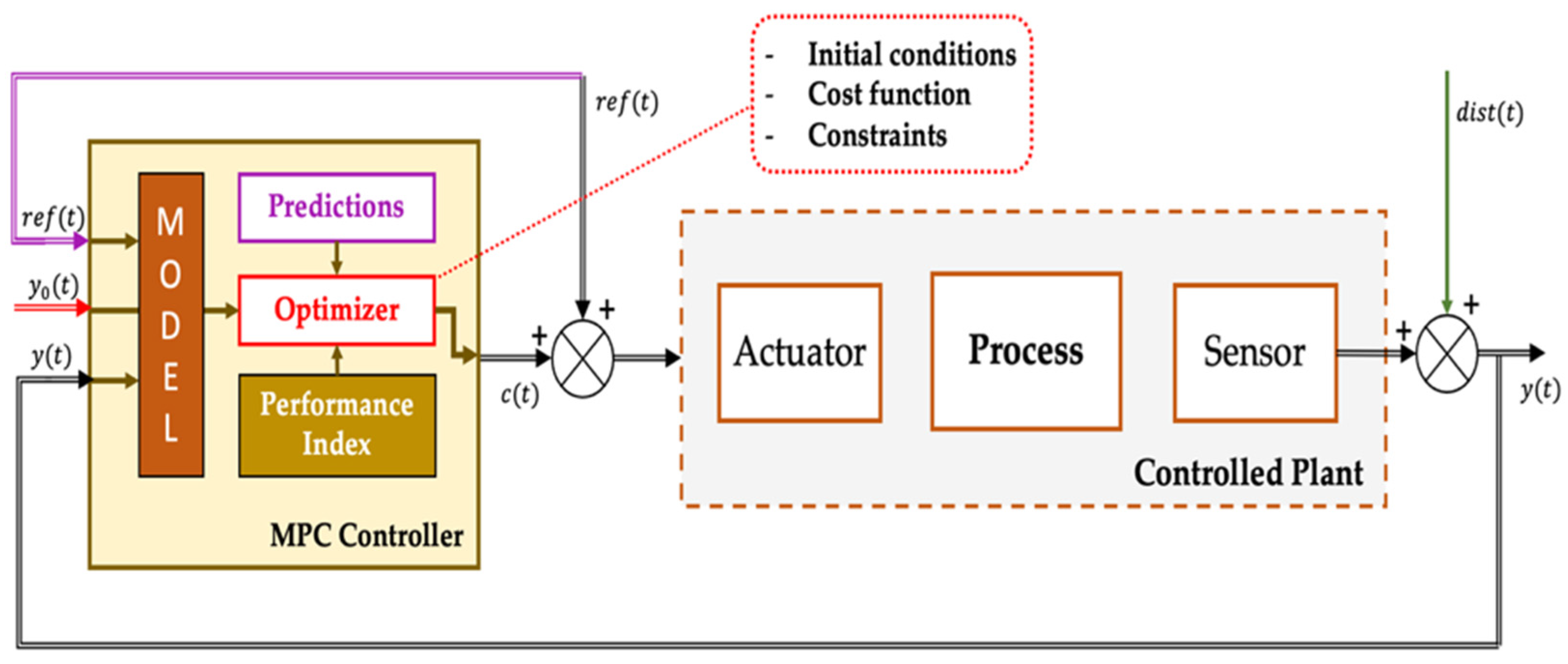
2.3.1. Model Predictive Control Concept

Model predictive control (MPC) is an advanced automatic control technique that is mostly useful for industrial applications. The MPC concept is based on using the linear or nonlinear dynamic model of the plant inside the controller in real time in order to anticipate the future behavior of the system. The main feature of MPC is that the output calculation must be solved online. The optimization process is based on the inputs/outputs of the system that minimize a cost function to predict the future. The prediction is executed from the internal model of the controller over a finite time window called the prediction horizon. The solution to the optimization problem is presented as a control vector. Using updated system data, the controller can solve the problem again in the next interval period, and therefore, MPC is also called moving horizon or receding horizon optimal control.

MPC solves an optimization problem, specifically a quadratic program (QP). It consists of the following three components: a state dynamic model; a cost function, which is the objective to achieve; and constraints, which are presented as boundaries to limit the future behavior of the inputs and outputs, where soft or hard constraints can be set.

MPC operates as follows: using the open-loop plant model and a chosen prediction horizon N, it calculates the set of future states ${\mathrm{x}}_{\mathrm{k}+1}, \dots \dots { \mathrm{x}}_{\mathrm{k}+\mathrm{N} }$and control inputs ${\mathrm{u}}_{\mathrm{k}}$,⋯, ${\mathrm{u}}_{\mathrm{k}+\mathrm{N}-1}$ that minimize the cost function subject to state and input constraints. Then, the first element ${\mathrm{u}}_{\mathrm{k}}$ in the set of calculated inputs is used as the input to the plant, and the sequence of calculations is repeated at the next sampling instant.

The MPC controller has shown its efficiency in applications with short sampling periods and has produced good results in terms of speed and accuracy in the field of numerical control [46]. Figure 5 shows the internal closed loop of MPC with the plant, and Figure 6 shows the internal behavior concept of MPC.

The standard cost function $\mathsf{\Theta }$ is usually the sum of four terms, each focusing on a particular aspect of controller performance.

Every term in $\mathsf{\Theta }$ represents an objective sub-function:

$$\mathsf{\Theta }\left({𝓏}_k\right)={\mathsf{\Theta }}_y\left({𝓏}_k\right)+{\mathsf{\Theta }}_u\left({𝓏}_k\right)+{\mathsf{\Theta }}_{\mathsf{\Delta }u}\left({𝓏}_k\right)+{\mathsf{\Theta }}_{\epsilon }\left({𝓏}_k\right)$$

(33)

where:

• ${\mathsf{\Theta }}_{\mathrm{y}}\left({𝓏}_{\mathrm{k}}\right)$: Cost function for output reference tracking;
• ${\mathsf{\Theta }}_{\mathrm{u}}\left({𝓏}_{\mathrm{k}}\right)$: Cost function for manipulated variable tracking;
• ${\mathsf{\Theta }}_{\mathsf{\Delta }\mathrm{u}}\left({𝓏}_{\mathrm{k}}\right)$: Cost function for manipulated variable movement suppression;
• ${\mathsf{\Theta }}_{\mathsf{\epsilon }}\left({𝓏}_{\mathrm{k}}\right)$: Cost function for constraint violation;
• ${𝓏}_{\mathrm{k}}$: The quadratic program.

In the presented case, the focus was on minimizing the two terms ${\mathsf{\Theta }}_{\mathrm{y}}\left({𝓏}_{\mathrm{k}}\right)$ and ${\mathsf{\Theta }}_{\mathrm{u}}\left({𝓏}_{\mathrm{k}}\right)$. In order to track the reference output, the error between the reference and the output signal should be minimized. Therefore, the second term was minimized so that the controller continues to select manipulated variables (MVs) at or near specified target values. In general, the problem statement is written as follows:

$$\underset{u_t, \dots , u_{t+N-1} }{\min }\left\{{\displaystyle \sum }_{k=0}^{N-1}{\Vert r\left(t\right)-y_{t+k}\Vert }^2+\rho {\Vert u_{t+k}-u_r\left(t\right)\Vert }^2\right\}$$

(34)

subject to:

• ${\mathrm{x}}_{\mathrm{t}+\mathrm{k}+1}= \mathrm{f}\left({\mathrm{x}}_{\mathrm{t}+\mathrm{k}},{ \mathrm{u}}_{\mathrm{t}+\mathrm{k}}\right)$, which represents the dynamic of the system;
• ${\mathrm{y}}_{\mathrm{t}+\mathrm{k}}= \mathrm{g}\left({\mathrm{x}}_{\mathrm{t}+\mathrm{k}},{ \mathrm{u}}_{\mathrm{t}+\mathrm{k}}\right)$, which represents the outputs of the system;
• ${\mathrm{u}}_{\min }\le { \mathrm{u}}_{\mathrm{t}+\mathrm{k}} \le { \mathrm{u}}_{\max }$;
• ${\mathrm{y}}_{\min }\le { \mathrm{y}}_{\mathrm{t}+\mathrm{k}} \le { \mathrm{y}}_{\max }$;
• ${\mathrm{x}}_{\mathrm{t}}= \mathrm{x}\left(\mathrm{t}\right)$, $\mathrm{k}=0,\dots , \mathrm{N}-1$, which represents state variables.

In the following, the design of linear and nonlinear MPC using MATLAB will be presented. The software provides several capabilities to solve energy modeling problems in research [47]. MATLAB’s model predictive control application allows the selection of suitable parameters to tune the controller according to the plant. Among the methods used, it can distinguish between standard linear MPC and nonlinear MPC, where the optimization problem is solved using a quadratic program (QP) at each control interval. The solution determines the manipulated variables (MVs) to be used in the plant until the next control interval. The definition of the cost function in the software according to this case is written as follows:

$$\mathsf{\Theta }\left({𝓏}_k\right)={\mathsf{\Theta }}_y\left({𝓏}_k\right)+{\mathsf{\Theta }}_u\left({𝓏}_k\right)$$

(35)

$$\mathsf{\Theta }\left({𝓏}_k\right)={\displaystyle \sum }_{j=1}^{n_y}{\displaystyle \sum }_{i=1}^p\left[{\left\{\frac{w_{i, j}^y}{s_j^y}\left[r_j\left(k+i|k\right)-y_j\left(k+i|k\right)\right]\right\}}^2+{\left\{\frac{w_{i, j}^y}{s_j^y}\left[u_j\left(k+i|k\right)-u_{j,target}\left(k+i|k\right)\right]\right\}}^2\right]$$

(36)

where $\mathrm{k}$ is the current control interval; $\mathrm{p}$ is the prediction horizon (number of intervals); and ${\mathrm{n}}_{\mathrm{y}}$is the number of plant output variables. ${𝓏}_{\mathrm{k}}$ is the quadratic program decision, given by:

$${𝓏}_k{}^T=\left[u{\left(k|k\right)}^T\dots \dots u{\left(k+p-1|k\right)}^T {\epsilon }_k \right]$$

(37)

where ${\mathrm{y}}_{\mathrm{j}}\left(\mathrm{k}+\mathrm{i}|\mathrm{k}\right)$ is the predicted value of the $\mathrm{j}$th plant output at the $\mathrm{i}$th prediction horizon step, in engineering units; ${\mathrm{r}}_{\mathrm{j}}\left(\mathrm{k}+\mathrm{i}|\mathrm{k}\right)$ is the reference value for the $\mathrm{j}$th plant output at the $\mathrm{i}$th prediction horizon step, in engineering units; ${\mathrm{s}}_{\mathrm{j}}^{\mathrm{y}}$ is the scale factor for the $\mathrm{j}$th plant output, in engineering units; and ${\mathrm{w}}_{\mathrm{i}, \mathrm{j}}^{\mathrm{y}} \mathrm{is} \mathrm{the}$ tuning weight for the $\mathrm{j}$th plant output at the $\mathrm{i}$th prediction horizon step (dimensionless).

2.3.2. Linear Model Predictive Control

Linear MPC is the traditional model, in which the basis of its cost function is a quadratic function; the model assumes linear dynamic systems, and extensive computation is not required to solve the optimization problem. The basic step to continue with linear MPC is to linearize the dynamic model of the quad-rotor, so the methodology is presented as follows:

• Linearization of the quad-rotor system

The aim of this section is to generate a linear state-space representation from the nonlinear model written in Equations (29) and (30). The nonlinear model is linearized around an equilibrium point ${\mathrm{X}}_{\mathrm{e}}$ (“hover position”), and linearization is performed on a simplified model, where small oscillations are considered as $\sin (\mathrm{angle})=\mathrm{angle}$ and $\cos (\mathrm{angle})=1$. Using a Taylor-series expansion, the new state-space representation after linearization is written in the following form:

$$\{\begin{array}{c}\overrightarrow{\dot{X}}=A\overrightarrow{X^{\prime }}+B\overrightarrow{u^{\prime }}\\ \overrightarrow{y}=C\overrightarrow{X^{\prime }}+D\overrightarrow{u^{\prime }}\end{array} \mathrm{where} \begin{array}{c}\overrightarrow{X^{\prime }}=\overrightarrow{X}-{\overrightarrow{X}}_e\\ \overrightarrow{u^{\prime }}=\overrightarrow{u}-{\overrightarrow{u}}_e\end{array}$$

(38)

where $\overrightarrow{\mathrm{X}}$is the “State vector” of $\left(\mathrm{n}\times 1\right)$, $\overrightarrow{\mathrm{u}}$ is the “Input (or control) vector” of $\left(\mathrm{m}\times 1\right)$, $\overrightarrow{\mathrm{y}}$ is the “Output vector” of $\left(\mathrm{p}\times 1\right)$, $\mathrm{A}$ is the “System Matrix” of $\left(\mathrm{n}\times \mathrm{n}\right)$, $\mathrm{B}$ is the “Input Matrix” of $\left(\mathrm{n}\times \mathrm{p}\right)$, $\mathrm{C}$ is the “Output Matrix” of $\left(\mathrm{q}\times \mathrm{n}\right)$, and $\mathrm{D}$ is the “Feed forward Matrix” of $\left(\mathrm{q}\times \mathrm{p}\right)$.

In the hover position, the state vector and input vector are represented as:

$$X_e={\left[\begin{array}{cc}\begin{array}{ccc}\begin{array}{ccc}{x}_e& y_e& z_e\end{array}& \begin{array}{ccc}0& 0& 0\end{array}& \begin{array}{ccc}0& 0& 0\end{array}\end{array}& \begin{array}{ccc}0& 0& 0\end{array}\end{array}\right]}^T$$

(39)

$$u_e={\left[\begin{array}{cc}\begin{array}{cc}mg& 0\end{array}& \begin{array}{cc}0& 0\end{array}\end{array}\right]}^T$$

(40)

After the linearization calculation, the following four matrices for the state-space representation are obtained:

$$A={\frac{\partial f\left(X,u\right)}{\partial X}|}_{\begin{array}{c}x=x_e\\ u=u_e\end{array}}=\left[\begin{array}{cccccccccccc}0& 0& 0& 0& 0& 0& 1& 0& 0& 0& 0& 0\\ 0& 0& 0& 0& 0& 0& 0& 1& 0& 0& 0& 0\\ 0& 0& 0& 0& 0& 0& 0& 0& 1& 0& 0& 0\\ 0& 0& 0& 0& 0& 0& 0& 0& 0& 1& 0& 0\\ 0& 0& 0& 0& 0& 0& 0& 0& 0& 0& 1& 0\\ 0& 0& 0& 0& 0& 0& 0& 0& 0& 0& 0& 1\\ 0& 0& 0& 0& g& 0& 0& 0& 0& 0& 0& 0\\ 0& 0& 0& -g& 0& 0& 0& 0& 0& 0& 0& 0\\ 0& 0& 0& 0& 0& 0& 0& 0& 0& 0& 0& 0\\ 0& 0& 0& 0& 0& 0& 0& 0& 0& 0& 0& 0\\ 0& 0& 0& 0& 0& 0& 0& 0& 0& 0& 0& 0\\ 0& 0& 0& 0& 0& 0& 0& 0& 0& 0& 0& 0\end{array}\right]$$

(41)

$$B={\frac{\partial f\left(X,u\right)}{\partial u}|}_{\begin{array}{c}x=x_e\\ u=u_e\end{array}}=\left[\begin{array}{cc}\begin{array}{cc}0& 0\\ 0& 0\end{array}& \begin{array}{cc}0& 0\\ 0& 0\end{array}\\ \begin{array}{cc}0& 0\\ \begin{array}{c}0\\ 0\\ \begin{array}{c}0\\ 0\\ \begin{array}{c}1/m\\ 0\\ 0\end{array}\end{array}\end{array}& \begin{array}{c}0\\ 0\\ \begin{array}{c}0\\ 0\\ \begin{array}{c}1/J_{xx}\\ 0\\ 0\end{array}\end{array}\end{array}\end{array}& \begin{array}{cc}0& 0\\ \begin{array}{c}0\\ 0\\ \begin{array}{c}0\\ 0\\ \begin{array}{c}0\\ 1/J_{yy}\\ 0\end{array}\end{array}\end{array}& \begin{array}{c}0\\ 0\\ \begin{array}{c}0\\ 0\\ \begin{array}{c}0\\ 0\\ 1/J_{zz}\end{array}\end{array}\end{array}\end{array}\end{array}\right]$$

(42)

Based on the chosen tracked outputs $\left[\mathrm{x} \mathrm{y} \mathrm{z} \varphi \mathsf{\theta } \mathsf{\psi }\right]$ and the control inputs, matrices C and D are the following:

$$C=\left[\begin{array}{cccccccccccc}1& 0& 0& 0& 0& 0& 0& 0& 0& 0& 0& 0\\ 0& 1& 0& 0& 0& 0& 0& 0& 0& 0& 0& 0\\ 0& 0& 1& 0& 0& 0& 0& 0& 0& 0& 0& 0\\ 0& 0& 0& 1& 0& 0& 0& 0& 0& 0& 0& 0\\ 0& 0& 0& 0& 1& 0& 0& 0& 0& 0& 0& 0\\ 0& 0& 0& 0& 0& 1& 0& 0& 0& 0& 0& 0\end{array}\right]$$

(43)

$$D=zero\left(6,4\right)$$

(44)

If the disturbance is taken into consideration, the matrix $\mathrm{dist}$ is added to the equation of the state space as follows:

$$\overrightarrow{\dot{X}}=A\overrightarrow{X^{\prime }}+B\overrightarrow{u^{\prime }}+dist\overrightarrow{d}$$

(45)

$$dist={\frac{\partial f\left(X,u,d\right)}{\partial d}|}_{\begin{array}{c}x=x_e\\ u=u_e\end{array}}$$

(46)

where $\overrightarrow{\mathrm{d}}$ is the vector of the disturbances applied to the quad-rotor. In the case presented in this paper, all disturbances are neglected.

• Design of Linear MPC for the Tello Quad-rotor System

The MATLAB Simulink software offers a block structure that defines the architecture of a basic linear MPC model, and the execution of this block is based on the injected identified parameters according to this dynamic system. Therefore, the dynamic system and linear MPC to track the following output variables $\left[\mathrm{x} \mathrm{y} \mathrm{z} \varphi \mathsf{\theta } \mathsf{\psi }\right]$ were designed. The process started by reconfiguring the main inputs and outputs of the controller. Figure 7 shows the necessary inputs and outputs for the MPC controller, where the inputs are:

-

mo: 6 measured outputs that represent the state vector $\left[\mathrm{x} \mathrm{y} \mathrm{z} \varphi \mathsf{\theta } \mathsf{\psi }\right]$;

-

md: 0 measured disturbances, where all disturbances applied to the quad-rotor are neglected.

The outputs are:

-

mv: 4 manipulated variables $\left[{\mathrm{u}}_1,{\mathrm{u}}_2,{\mathrm{u}}_3,{\mathrm{u}}_4\right]$, which represent the input control variables.

In the MPC plant model, different recommendations can be taken into consideration, depending on the characteristics of the dynamic system: in this case, the constraints, the weights, and the control horizon were set as presented in

Table 3. The required parameters of MPC for the Tello quad-rotor.

MPC Parameters
Sample time ($T_s$)	0.1 s
Prediction horizon (P)	20 s
Control horizon (M)	3 s
MPC Constraints
Boundaries of $u_1$	[−10–12] Nm
Boundaries of $u_2$	[−10–12] Nm
Boundaries of $u_3$	[−10–12] Nm
Boundaries of $u_4$	[−10–12] Nm
MPC Weights
Translation motion along $x$	1
Translation motion along $y$	1
Translation motion along $z$	1
Pitch motion along $\varphi$	0.1
Roll motion along $\theta$	0.1
Yaw motion along $\psi$	0.1

. The weight refers to the priority of a variable, where a high weight indicates a higher tracking priority.

Figure 7. MPC controller inputs and outputs.

Figure 7. MPC controller inputs and outputs.

2.3.3. Nonlinear Model Predictive Control

The principle of nonlinear model predictive control is the same as the linear one, but the key differences are:

• The prediction model can be nonlinear and include time-varying parameters.
• The equality and inequality constraints can be nonlinear.
• The scalar cost function to be minimized can be a nonquadratic (linear or nonlinear) function of the decision variables.

When the dynamic model is linear, a global analytical solution to the optimization problem exists and is relatively simple to determine [27]. However, when this model is nonlinear, it is not certain that the optimization algorithm converges to the global analytical solution, and if a solution is found, there is no certainty that it is fast enough. Indeed, the use of a nonlinear model involves solving a nonlinear optimization problem, whose complexity is related to the degree of accuracy of the model.

Several numerical techniques were developed to guarantee the convergence of the optimization algorithm towards an approximation of the overall optimum. While some of these methods, such as Eleanor’s method, have proven their efficiency, they are not appropriate for the control of drones due to their running time. Among the techniques that can be applied to the vehicles are the gradient method, the sequential quadratic programming method, or the particle swarm method. Some techniques are also based on the approximation of certain signals by their Taylor-series expansion [28,29,30,48,49].

While traditional linear MPC controllers optimize control actions to minimize a quadratic cost function, nonlinear MPC controllers support generic custom cost functions. For example, the cost function can be specified as a combination of linear or nonlinear functions of the system states and inputs. To improve computational efficiency, it is also possible to specify an analytical Jacobean for the custom cost function [50].

Using a custom cost function, the algorithm of NLMPC will be able to maximize profitability and minimize energy consumption.

• Design of Nonlinear MPC for the Tello quad-rotor system

As presented in the previous part for linear MPC, the design of NLMPC was performed in the MATLAB Simulink environment, which already has a basic architecture block function of such a controller. It is necessary to reconfigure the internal structure according to the system and tune the main parameters to achieve high performance. According to the nonlinear dynamic system of the Tello quad-rotor, the controller should receive different input signals: the reference trajectory, 12 state variables, and the last 4 manipulated variables that represent the 4 control input variables$\left[{\mathrm{u}}_1^{\prime },{\mathrm{u}}_2^{\prime },{\mathrm{u}}_3^{\prime },{\mathrm{u}}_4^{\prime }\right]$, as presented in Figure 8. In this case, the gyroscopic effect and the other disturbances applied to the system were neglected, whereas outputs received the 4 newly updated manipulated variables.

The design process for NLMPC is as follows: an object function nlobj is created in the internal block by setting the necessary parameters, and using the nlmpc function, a nonlinear MPC controller is designed. A drawback of nonlinear controllers is the long time required for simulation, so to avoid this issue and guarantee high performance for the system, an algorithm to calculate the Jacobean function was inserted into the controller block function since the Jacobean function guarantees fast and efficient simulation.

Table 4. The required parameters of nonlinear MPC for Tello quad-rotor.

Nonlinear MPC Parameters
Sample time ($T_s$)	0.1 s
Prediction Horizon (P)	18 s
Control Horizon (M)	3 s
Nonlinear MPC Constraints
Boundaries of $u_1$	[0–12] Nm
Boundaries of $u_2$	[0–10] Nm
Boundaries of $u_3$	[0–10] Nm
Boundaries of $u_4$	[0–10] Nm
Nonlinear MPC Weights
Translation motion along $x$	1
Translation motion along $y$	1
Translation motion along $z$	1
Pitch motion along $\varphi$	1
Roll motion along $\theta$	1
Yaw motion along $\psi$	1

identifies the necessary parameters for nonlinear MPC that fit the Tello quad-rotor. The weight parameter in the controller refers to the priorities of the variables to track. Generally, in the quad-rotor, a higher priority was given to position variables rather than orientation variables, since the aim was to obtain the best performance. So, the higher priorities for all six variables were set.

3. Results and Discussion

In this section, several simulations for three different trajectories are presented to validate the comparison between linear and nonlinear MPC based on the performance analyses of the following inputs and outputs:

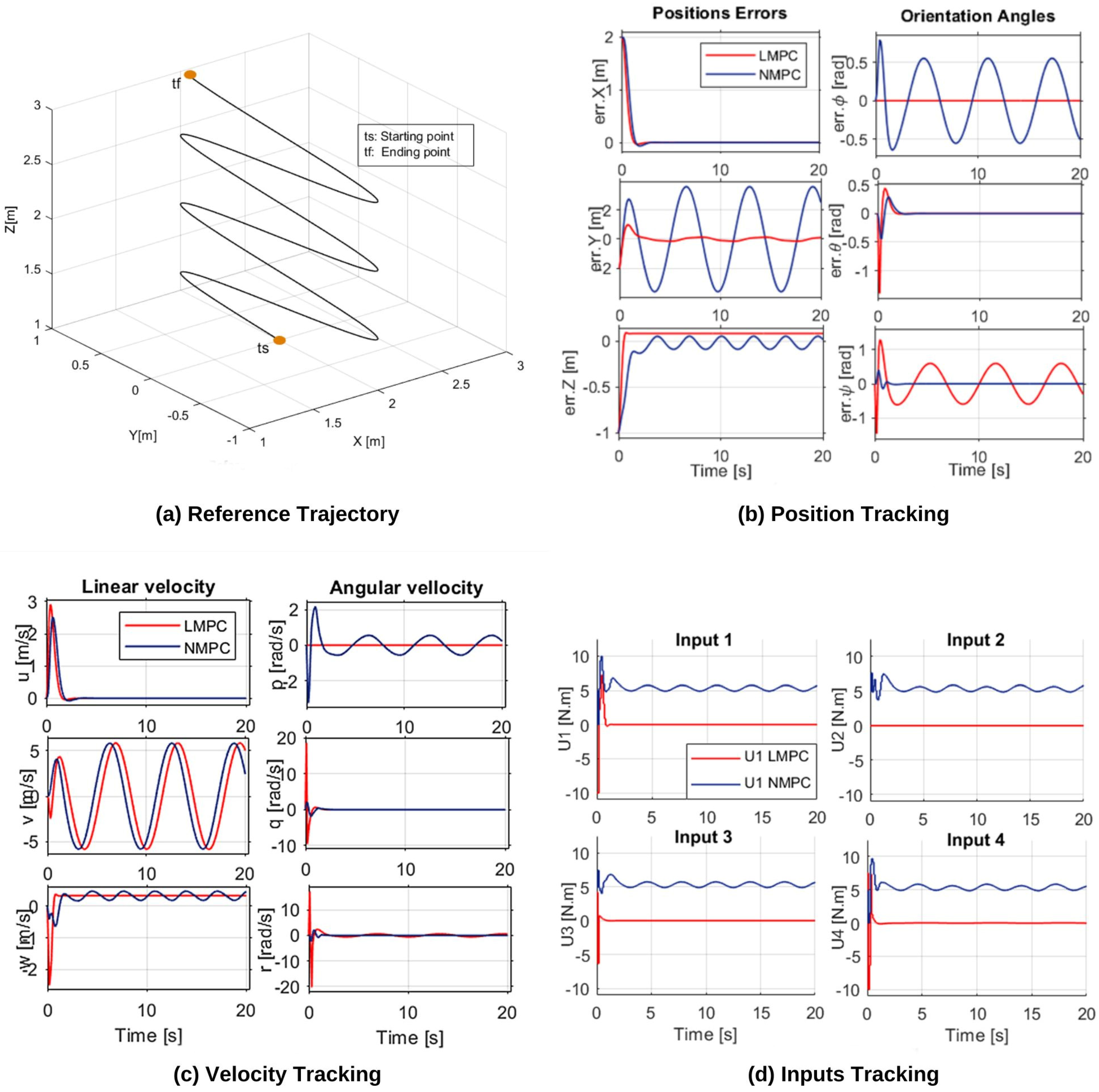
• Error position tracking;
• Velocity tracking;
• Control input tracking.

The design of the linear and nonlinear dynamic models of the drone, in addition to the linear and nonlinear MPC models, were designed in MATLAB Simulink, where different functions were written in MATLAB Script as follows: the trajectory function, which provides the control loop with the desired reference trajectory, and the Jacobean function, which guarantees a solution to the optimization problem while avoiding singularities.

Three generated trajectories are defined: the first represents the straight curvature motion of the drone, the second trajectory is presented as a circular motion, and the third trajectory is a helical motion. The initial states for both controllers were set as follows: X_i = [0 2 2 0 0 0 0 0 0 0 0 0]^T.

For linear MPC, the control input bounds were set between a minimum value of −10 and a maximum value of 12, as presented in Table 3. This choice gives the controller more freedom to track the trajectory than if the minimum value is set to 0. The controller will behave in an aggressive scenario. For nonlinear MPC, the control input boundaries were set between a minimum value of 0 and a maximum value of 12. Another setting was used for control input tracking so that, for nonlinear MPC, the tracking of control inputs can be implemented successfully, so the track values were set to [4.9 4.9 4.9 4.9], while for linear MPC, this option was neglected because it will definitely disturb the controller in achieving the highest-priority task, which is tracking the position and orientation outputs. From the first attempt and without looking at the simulation results, the recognition of these limitations shows that nonlinear MPC is more flexible than linear MPC in terms of setting conditions.

3.1. Straight Curvature Reference Trajectory

Figure 9 presents the simulation results of the straight curvature reference trajectory, error position tracking, velocity tracking, and control input tracking for linear and nonlinear MPC. In Figure 9, it can be observed that, for error position tracking, LMPC performs better regarding the three axes, X, Y, and Z, whereas for orientation angles, the signal is disturbed compared to NLMPC, where the oscillations are minimized. These oscillations describe the instability of the drone. Additionally, at the level of tracking velocity, both controllers behave nearly the same, but NLMPC is always able to minimize the peak amplitude of the oscillations. From the energy profile perspective, a comparison of the control input tracking shows that both controllers reach the maximum and the minimum boundaries set earlier. To know which controller is using more torque, the mean value of $\mathsf{\Delta }u$ for every execution is calculated, and the results are presented in

Table 5. Calculation of the average control effort value and the execution time.

Trajectory/Controller	1st Trajectory		2nd Trajectory		3rd Trajectory
Δu [Nm]/ ExTime [ms]	Δu	ExTime	Δu	ExTime	Δu	ExTime
LMPC	3.1678	64	2.7054	63	1.4229	62
NLMPC	5.9188	6.8	5.2379	6	4.8955	5.7

.

3.2. Circular Reference Trajectory

Figure 10 presents the simulation results with a circular motion as the reference trajectory. The figure clearly displays the differences between control methods, where it is obvious that NLMPC tracks the positions and velocities with stable behavior, whereas oscillations are more evident with LMPC; otherwise, NLMPC has succeeded in minimizing them. In addition, at the control input tracking level, LMPC uses the maximum and minimum boundaries, so it can reach the minimum value of 10 Nm, whereas NLMPC behaves well with a limited boundary with a minimum value of 0 Nm. NLMPC is also able to track the set target control inputs [4.9 4.9 4.9 4.9].

3.3. Helical Reference Trajectory

Figure 11 presents the simulation results with a helical motion as the reference trajectory. This motion is typical in real life, where the motion depends on the three axes simultaneously. NLMPC succeeds in tracking the three positions smoothly and with the minimum peak amplitude for orientation tracking, but an overshoot appears in the first two seconds for velocity tracking. NLMPC also provides good results, as the tracking of control inputs is better achieved by NLMPC compared to LMPC. LMPC always uses all boundaries to execute suitable control behavior.

3.4. Performance measurements $\mathsf{\Delta }u$and ExTime

In order to analyze the energy profiles of both controllers, calculations of the mean average value of the control effort $\mathsf{\Delta }u$ and the execution time of the simulation $E{x}_{Time}$ were made.

Table 5 shows the results of the two values when every trajectory is executed. These two parameters identify the energy consumption for both controllers: regarding the execution time, LMPC is very slow compared to NLMPC, while the average control effort for LMPC is less than the control effort required by NLMPC, with average differences. This can be explained by the fact that NLMPC has different missions to achieve, as it not only tracks the trajectory but also tries to maintain a target value for the control inputs. A solution can be attempted in the future by optimizing a cost function that minimizes the energy consumption of the drone by minimizing the applied control efforts directed to the four motors.

The calculation of $\mathsf{\Delta }u$ was carried out by the mean function, whereas the execution simulation time was calculated by the timeit function.

4. Summary and Conclusions

This paper presents a methodology to design an MPC controller with the purpose of tracking the trajectory of a quad-rotor system while considering minimum energy consumption. The dynamic mathematical model for the quad-rotor is described in the first section, while in the second section, a theoretical comparison between linear and nonlinear MPC is presented, which looks at the efficiency of both control laws, especially regarding the energy profile. The design of both controller models was built and configured using MATLAB Script and Simulink, and the controllers were simulated with the execution of three different trajectories to see the resulting behavior. In conclusion, NLMPC can provide very promising results compared to LMPC, which is not flexible and has different limitations in the drone control field.

This paper is a case study on the customized development of a powerful embedded control system. This control system is intended to control a Tello EDU quad-rotor model. The quad-rotor already has a basic embedded system that fulfills simple commands for take-off and landing motions but with low accuracy and stability. This work provides completely new model designs for linear and nonlinear MPC controllers intended to be used for indoor applications using the Tello drone. Simulations show that NLMPC accurately tracks the reference trajectories with faster execution time but higher energy consumption compared to LMPC. On the other hand, LMPC consumes low energy but with very strict limitations regarding the control inputs.

One of the limitations regarding the obtained results is that although it is clear that NLMPC is efficient in tracking trajectories and execution time, it consumes more energy than LMPC. This issue can be improved in the future by generating a cost function that optimizes the power supply by minimizing the angular velocity of the rotors while executing a motion.

Another limitation is that the Tello drone is a closed system and accepts commands only via Wi-Fi. So, the presented control system will be implemented in a master controller. For future work, the main goal is to build a master controller hardware-embedded system for a Tello quad-rotor. The main advantage of this hardware is to achieve the drone task while forcing the drone to decrease its energy consumption, which will result in a longer flying time.

References

1. Barnhart, R.K.; Hottman, S.B.; Marshall, D.M.; Shappee, E. Introduction to Unmanned Aircraft Systems, 1st ed.; CRC Press: Boca Raton, FL, USA, 2016. [Google Scholar] [CrossRef]
2. Nonami, K.; Kendoul, F.; Suzuki, S.; Wang, W.; Nakazawa, D. Autonomous Flying Robots: Unmanned Aerial Vehicles and Micro Aerial Vehicles; Springer: Tokyo, Japan, 2010. [Google Scholar] [CrossRef]
3. Padfield, G.D.; Kluever, C.A.; Young, T.M.; Keane, A.J.; Sóbester, A.; Scanlan, J.P. Design of Unmanned Aerial Systems. In Design of Unmanned Aerial Systems; Wiley: New York, NY, USA, 2020. [Google Scholar] [CrossRef]
4. Dalamagkidis, K. Classification of Uavs; Springer: Dordrecht, The Netherlands, 2014. [Google Scholar] [CrossRef]
5. Idrissi, M.; Salami, M.; Annaz, F. A Review of Quadrotor Unmanned Aerial Vehicles: Applications, Architectural Design and Control Algorithms. J. Intell. Robot. Syst. 2022, 104, 22. [Google Scholar] [CrossRef]
6. Jacewicz, M.; Żugaj, M.; Głębocki, R.; Bibik, P. Quadrotor Model for Energy Consumption Analysis. Energies 2022, 15, 7136. [Google Scholar] [CrossRef]
7. Zhang, X.; Li, X.; Wang, K.; Lu, Y. A Survey of Modelling and Identification of Quadrotor Robot. Abstr. Appl. Anal. 2014, 2014, 320526. [Google Scholar] [CrossRef]
8. Ye, J.; Wang, J.; Lv, P. Mutual Aerodynamic Interference Mechanism Analysis of an “X” Configuration Quadcopter. Aerospace 2021, 8, 349. [Google Scholar] [CrossRef]
9. Balestrieri, E.; Daponte, P.; De Vito, L.; Lamonaca, F. Sensors and Measurements for Unmanned Systems: An Overview. Sensors 2021, 21, 1518. [Google Scholar] [CrossRef]
10. Guan, S.; Zhu, Z.; Wang, G. A Review on UAV-Based Remote Sensing Technologies for Construction and Civil Applications. Drones 2022, 6, 117. [Google Scholar] [CrossRef]
11. Barbaraci, G. Modeling and control of a quadrotor with variable geometry arms. J. Unmanned Veh. Syst. 2015, 3, 35–57. [Google Scholar] [CrossRef]
12. Tahir, Z.; Jamil, M.; Liaqat, S.A.; Mubarak, L.; Tahir, W.; Gilani, S.O. State Space System Modeling of a Quad Copter UAV. Indian J. Sci. Technol. 2016, 9. [Google Scholar] [CrossRef]
13. Chovancová, A.; Fico, T.; Chovanec, Ľ.; Hubinsk, P. Mathematical Modelling and Parameter Identification of Quadrotor (a survey). Procedia Eng. 2014, 96, 172–181. [Google Scholar] [CrossRef] [Green Version]
14. Mokhtari, M.R.; Cherki, B. A new robust control for minirotorcraft unmanned aerial vehicles. ISA Trans. 2015, 56, 86–101. [Google Scholar] [CrossRef]
15. Bodó, Z.; Lantos, B. Modeling and Control of Outdoor Quadrotor UAVs. In Proceedings of the SISY 2018—IEEE 16th International Symposium on Intelligent Systems and Informatics, Subotica, Serbia, 13–15 September 2018; pp. 111–116. [Google Scholar] [CrossRef]
16. Ducard, G.J.; Allenspach, M. Review of designs and flight control techniques of hybrid and convertible VTOL UAVs. Aerosp. Sci. Technol. 2021, 118, 107035. [Google Scholar] [CrossRef]
17. Chand, A.N.; Kawanishi, M.; Narikiyo, T. Adaptive pole placement pitch angle control of a flapping-wing flying robot. Adv. Robot. 2016, 30, 1039–1049. [Google Scholar] [CrossRef]
18. Chen, N.; Song, F.; Li, G.; Sun, X.; Ai, C. An adaptive sliding mode backstepping control for the mobile manipulator with nonholonomic constraints. Commun. Nonlinear Sci. Numer. Simul. 2013, 18, 2885–2899. [Google Scholar] [CrossRef]
19. Bogdanov, A.; Carlsson, M.; Harvey, G.; Hunt, J.; Kieburtz, D.; van der Merwe, R.; Wan, E. State-dependent riccati equation control of a small unmanned helicopter. In Proceedings of the AIAA Guidance, Navigation, and Control Conference and Exhibit, Austin, TX, USA, 11–14 August 2003. [Google Scholar] [CrossRef] [Green Version]
20. Raffo, G.V.; Ortega, M.G.; Rubio, F.R. Robust Nonlinear Control for Path Tracking of a Quad-Rotor Helicopter. Asian J. Control. 2015, 17, 142–156. [Google Scholar] [CrossRef]
21. How, J.P.; Frazzoli, E.; Chowdhary, G.V. Linear Flight Control Techniques for Unmanned Aerial Vehicles; Springer: Dordrecht, The Netherlands, 2015. [Google Scholar] [CrossRef]
22. Khan, N.; Ullah, F.U.M.; Afnan; Ullah, A.; Lee, M.Y.; Baik, S.W. Batteries State of Health Estimation via Efficient Neural Networks With Multiple Channel Charging Profiles. IEEE Access 2020, 9, 7797–7813. [Google Scholar] [CrossRef]
23. Kim, J.; Baek, S.; Jeon, S.; Cha, H. DynLiB: Maximizing Energy Availability of Hybrid Li-Ion Battery Systems. IEEE Trans. Comput. Des. Integr. Circuits Syst. 2022, 41, 3850–3861. [Google Scholar] [CrossRef]
24. Bodó, Z.; Lantos, B. Integrating Backstepping Control of Outdoor Quadrotor UAVs. Period. Polytech. Electr. Eng. Comput. Sci. 2019, 63, 122–132. [Google Scholar] [CrossRef]
25. Gao, F.; Wang, L.; Wang, K.; Wu, W.; Zhou, B.; Han, L.; Shen, S. Optimal Trajectory Generation for Quadrotor Teach-and-Repeat. IEEE Robot. Autom. Lett. 2019, 4, 1493–1500. [Google Scholar] [CrossRef]
26. Ryzerobotics. User Manual 2018.09; Ryze Robotics: Shenzhen, China, 2018; 22p. [Google Scholar]
27. Ru, P.; Subbarao, K. Nonlinear Model Predictive Control for Unmanned Aerial Vehicles. Aerospace 2017, 4, 31. [Google Scholar] [CrossRef]
28. Ławryńczuk, M.; Nebeluk, R. Computationally Efficient Nonlinear Model Predictive Control Using the L1 Cost-Function. Sensors 2021, 21, 5835. [Google Scholar] [CrossRef]
29. Rubio, A.A.; Seuret, A.; Mannisi, A.; Ariba, Y.; Arce, A. Optimal control strategies for load carrying drones. In Delays and Networked Control Systems; Springer: Cham, Switzerland, 2016; Volume 6, pp. 183–197. [Google Scholar] [CrossRef] [Green Version]
30. Al Younes, Y.; Barczyk, M. Nonlinear Model Predictive Horizon for Optimal Trajectory Generation. Robotics 2021, 10, 90. [Google Scholar] [CrossRef]
31. Benotsmane, R.; Reda, A.; Vasarhelyi, J. Model Predictive Control for Autonomous Quadrotor Trajectory Tracking. In Proceedings of the 2022 23rd International Carpathian Control Conference (ICCC 2022), Bolzano, Italy, 27 June–1 July 2022; pp. 215–220. [Google Scholar] [CrossRef]
32. Roy, R.; Islam, M.; Sadman, N.; Mahmud, M.; Gupta, K.; Ahsan, M. A Review on Comparative Remarks, Performance Evaluation and Improvement Strategies of Quadrotor Controllers. Technologies 2021, 9, 37. [Google Scholar] [CrossRef]
33. Hongwei, M.; Ali, S.M.; Liwei, Q.; Farid, G. A Review on Linear and Nonlinear Control Techniques for Position and Attitude Control of a Quadrotor. Control. Intell. Syst. 2017, 45, 43–57. [Google Scholar] [CrossRef]
34. Emran, B.J.; Najjaran, H. A review of quadrotor: An underactuated mechanical system. Annu. Rev. Control. 2018, 46, 165–180. [Google Scholar] [CrossRef]
35. Araar, O.; Aouf, N. Full linear control of a quadrotor UAV, LQ vs H∞. In Proceedings of the 2014 UKACC International Conference on Control (CONTROL 2014), Loughborough, UK, 9–11 July 2014; pp. 133–138. [Google Scholar] [CrossRef]
36. Koszewnik, A. The Parrot UAV Controlled by PID Controllers. Acta Mech. Autom. 2014, 8, 65–69. [Google Scholar] [CrossRef] [Green Version]
37. Rawlings, J.B.; Meadows, E.S.; Muske, A.D.K.R. Nonlinear Model Predictive Control: A Tutorial and Survey. IFAC Proc. Vol. 1994, 27, 185–197. [Google Scholar] [CrossRef]
38. Isidori, A.; Marconi, L.; Serrani, A. Robust nonlinear motion control of a helicopter. IEEE Trans. Autom. Control 2003, 48, 413–426. [Google Scholar] [CrossRef]
39. Qin, S.J.; Badgwell, T.A. An Overview of Nonlinear Model Predictive Control Applications. In Nonlinear Model Predictive Control; Birkhäuser: Basel, Switzerland, 2000; pp. 369–392. [Google Scholar] [CrossRef] [Green Version]
40. Bentarzi, H.; Dekhandji, F.Z.; Saibi, A.; Boushaki, R.; Belaidi, H. Backstepping Control of Drone. Eng. Proc. 2022, 14, 4. [Google Scholar] [CrossRef]
41. Lee, K.U.; Choi, Y.H.; Park, J.B. Backstepping Based Formation Control of Quadrotors with the State Transformation Technique. Appl. Sci. 2017, 7, 1170. [Google Scholar] [CrossRef]
42. Herrera, M.; Chamorro, W.; Gómez, A.P.; Camacho, O. Sliding Mode Control: An Approach to Control a Quadrotor. In Proceedings of the 2015 Asia-Pacific Conference on Computer-Aided System Engineering (APCASE 2015), Quito, Ecuador, 14–16 July 2015; pp. 314–319. [Google Scholar] [CrossRef]
43. Doan, Q.V.; Vo, A.T.; Le, T.D.; Kang, H.-J.; Nguyen, N.H.A. A Novel Fast Terminal Sliding Mode Tracking Control Methodology for Robot Manipulators. Appl. Sci. 2020, 10, 3010. [Google Scholar] [CrossRef]
44. Lungu, M.; Lungu, R. Adaptive backstepping flight control for a mini-UAV. Int. J. Adapt. Control Signal Process. 2012, 27, 635–650. [Google Scholar] [CrossRef]
45. Deng, Z.; Zhu, H.; Lin, S. Adaptive Sliding Mode Control Method for Reconfigurable Modular Robots under Dynamic Constraints. Acad. J. Manuf. Eng. 2020, 18, 16–20. [Google Scholar]
46. Camacho, C.B.E.F. Model Predictive Control; Springer: London, UK, 2000. [Google Scholar] [CrossRef]
47. Mądziel, M.; Jaworski, A.; Kuszewski, H.; Woś, P.; Campisi, T.; Lew, K. The Development of CO2 Instantaneous Emission Model of Full Hybrid Vehicle with the Use of Machine Learning Techniques. Energies 2022, 15, 142. [Google Scholar] [CrossRef]
48. Kamel, M.; Burri, M.; Siegwart, R. Linear vs Nonlinear MPC for Trajectory Tracking Applied to Rotary Wing Micro Aerial Vehicles. IFAC-PapersOnLine 2017, 50, 3463–3469. [Google Scholar] [CrossRef]
49. Domański, P.D. Performance Assessment of Predictive Control—A Survey. Algorithms 2020, 13, 97. [Google Scholar] [CrossRef] [Green Version]
50. Benotsmane, R.; Vásárhelyi, J. Nonlinear Model Predictive Control for Autonomous Quadrotor Trajectory Tracking. In Lecture Notes in Mechanical Engineering, 4th ed.; Jármai, K., Cservenák, Á., Eds.; Springer: Cham, Switzerland, 2022; pp. 24–34. [Google Scholar] [CrossRef]
Figure 1. The possible motions of quad-rotor with cross configuration.
Energies 15 09207 g001
Figure 3. Basic components of the Tello drone.
Energies 15 09207 g003
Figure 4. Modeling frame assignments for the Tello quad-rotor [31].
Energies 15 09207 g004
Figure 5. MPC closed control loop.
Energies 15 09207 g005
Figure 6. Concept of Model Predictive Control.
Energies 15 09207 g006
Figure 8. Nonlinear MPC controller inputs and outputs.
Energies 15 09207 g008
Figure 9. Straight curvature trajectory.
Energies 15 09207 g009
Figure 10. Circular reference trajectory.
Energies 15 09207 g010
Figure 11. Circular reference trajectory.
Energies 15 09207 g011