Author Contributions
Conceptualization, P.S. and R.-J.W.; methodology, P.S. and R.-J.W.; software, P.S.; validation, P.S. and R.-J.W.; formal analysis, P.S.; investigation, P.S.; resources, P.S. and R.-J.W.; data curation, P.S.; writing—original draft preparation, P.S.; writing—review and editing, P.S. and R.-J.W.; visualization, P.S.; supervision, R.-J.W. All authors have read and agreed to the published version of the manuscript.
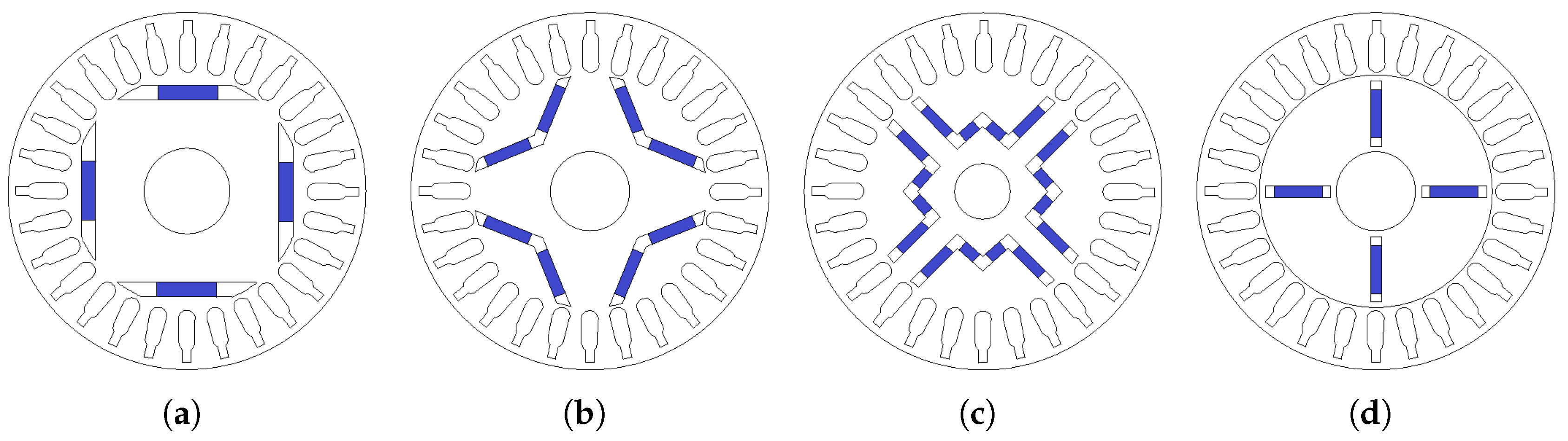
Figure 1.
Various LSPMSM rotor layouts: (a) radial-type; (b) V-type; (c) W-type; (d) spoke-type.
Figure 1.
Various LSPMSM rotor layouts: (a) radial-type; (b) V-type; (c) W-type; (d) spoke-type.
Figure 2.
Various torque components during the asynchronous operation of a LSPMSM.
Figure 2.
Various torque components during the asynchronous operation of a LSPMSM.
Figure 3.
Braking torque for various magnet volumes.
Figure 3.
Braking torque for various magnet volumes.
Figure 4.
Finding .
Figure 4.
Finding .
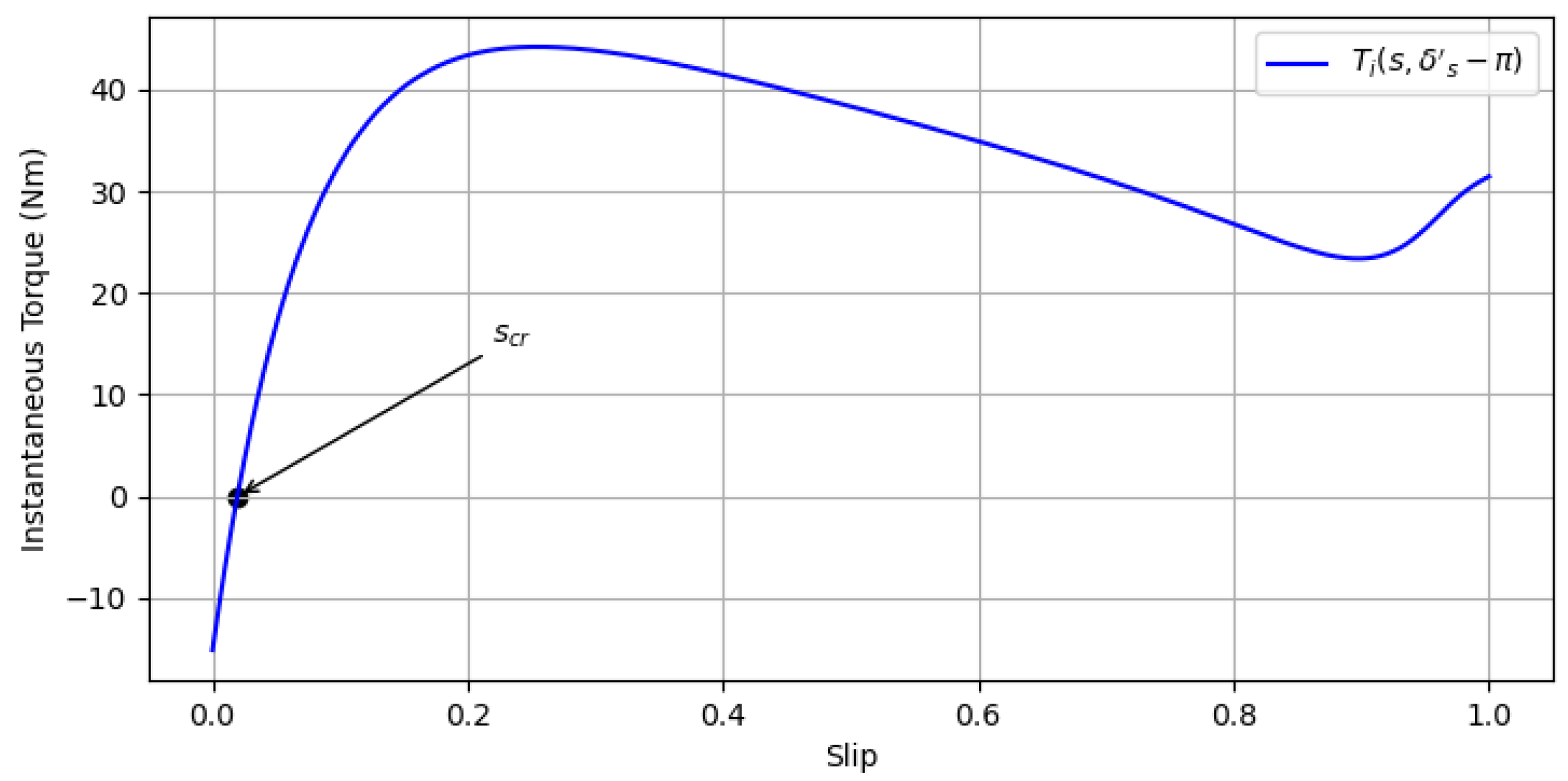
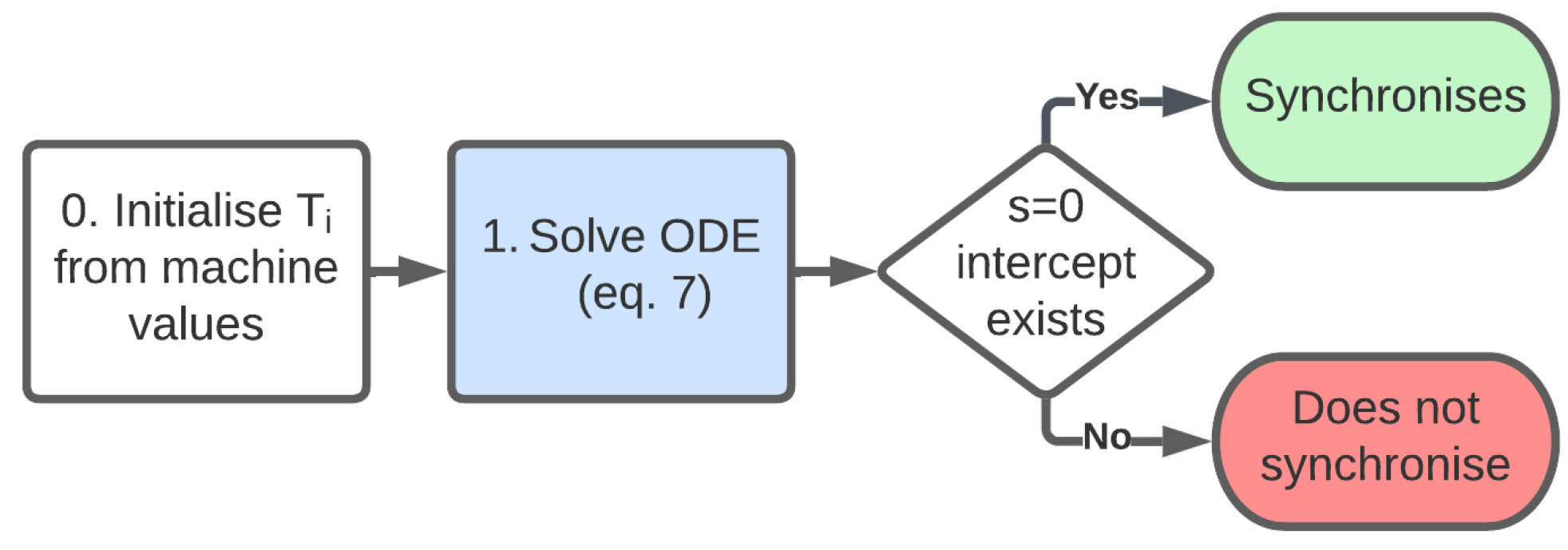
Figure 5.
Finding the critical slip.
Figure 5.
Finding the critical slip.
Figure 6.
Slip as a function of .
Figure 6.
Slip as a function of .
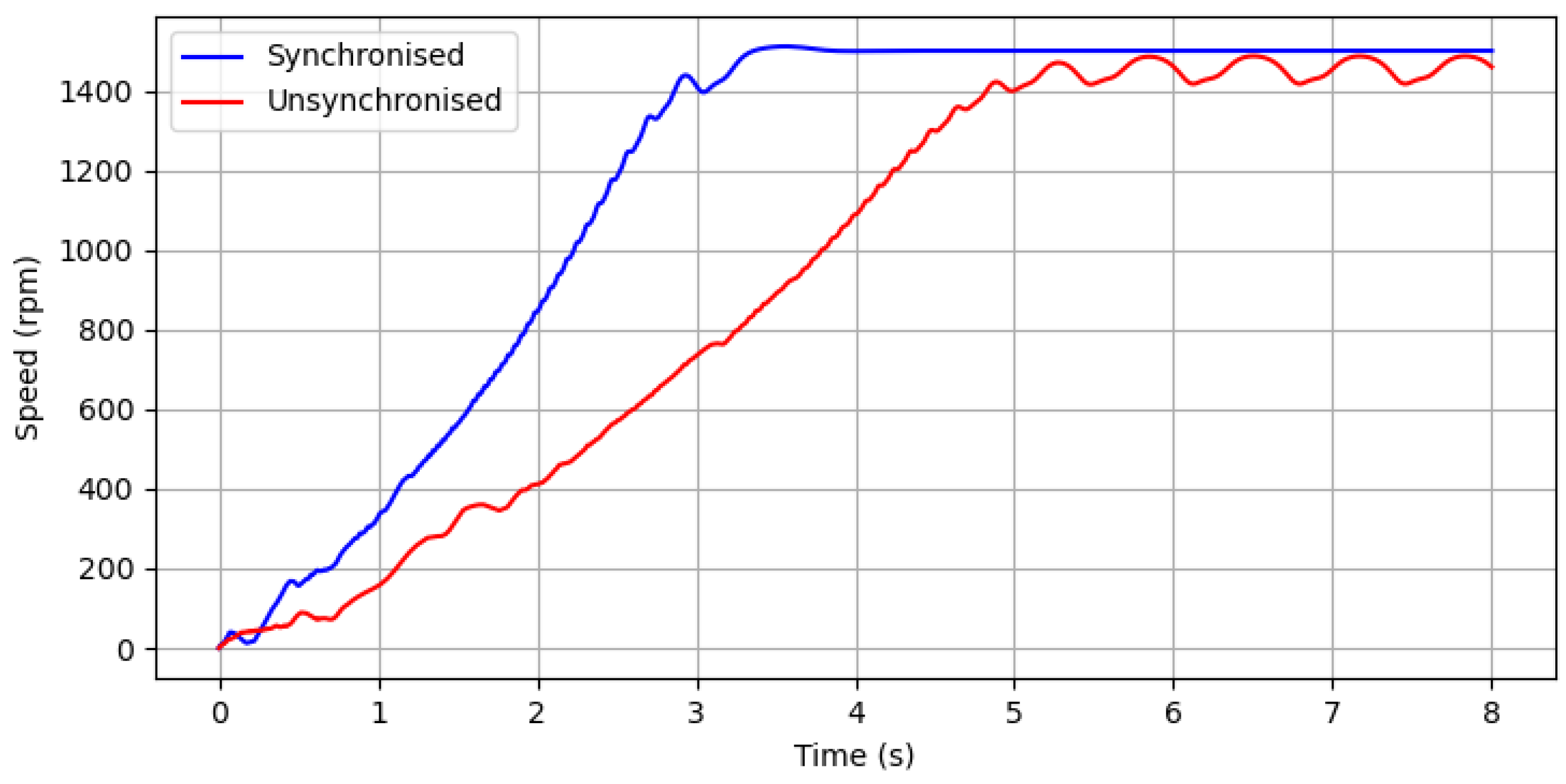
Figure 7.
Speed vs. time graphs for a synchronized and un-synchronized motor.
Figure 7.
Speed vs. time graphs for a synchronized and un-synchronized motor.
Figure 8.
Various (Rabbi et al. [
8], Chama et al. [
9], Soulard et al. [
19]) analytical cage torque curves for the Radial 1 design.
Figure 8.
Various (Rabbi et al. [
8], Chama et al. [
9], Soulard et al. [
19]) analytical cage torque curves for the Radial 1 design.
Figure 9.
Average torque difference of various (Rabbi et al. [
8], Chama et al. [
9], Soulard et al. [
19]) analytical
s from target
for each motor design.
Figure 9.
Average torque difference of various (Rabbi et al. [
8], Chama et al. [
9], Soulard et al. [
19]) analytical
s from target
for each motor design.
Figure 10.
Box plot of average torque difference of various (Rabbi et al. [
8], Chama et al. [
9], Soulard et al. [
19]) analytical
equations from target
for the design set.
Figure 10.
Box plot of average torque difference of various (Rabbi et al. [
8], Chama et al. [
9], Soulard et al. [
19]) analytical
equations from target
for the design set.
Figure 11.
Box plot of average torque difference of various (Rabbi et al. [
8], Chama et al. [
9], Soulard et al. [
19]) analytical
equations from target
for the region
for the design set.
Figure 11.
Box plot of average torque difference of various (Rabbi et al. [
8], Chama et al. [
9], Soulard et al. [
19]) analytical
equations from target
for the region
for the design set.
Figure 12.
for various (Rabbi et al. [
8], Tang [
17], Soulard et al. [
19])
cases.
Figure 12.
for various (Rabbi et al. [
8], Tang [
17], Soulard et al. [
19])
cases.
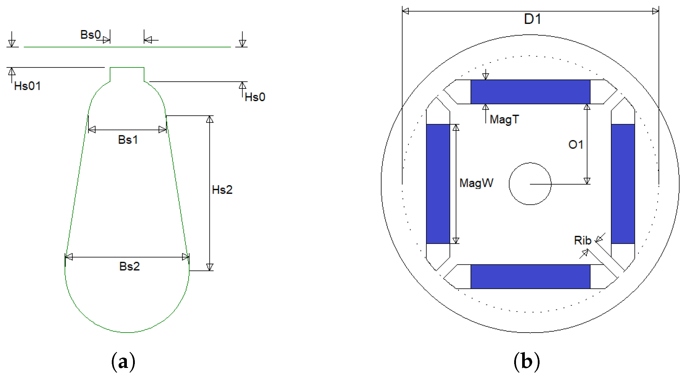
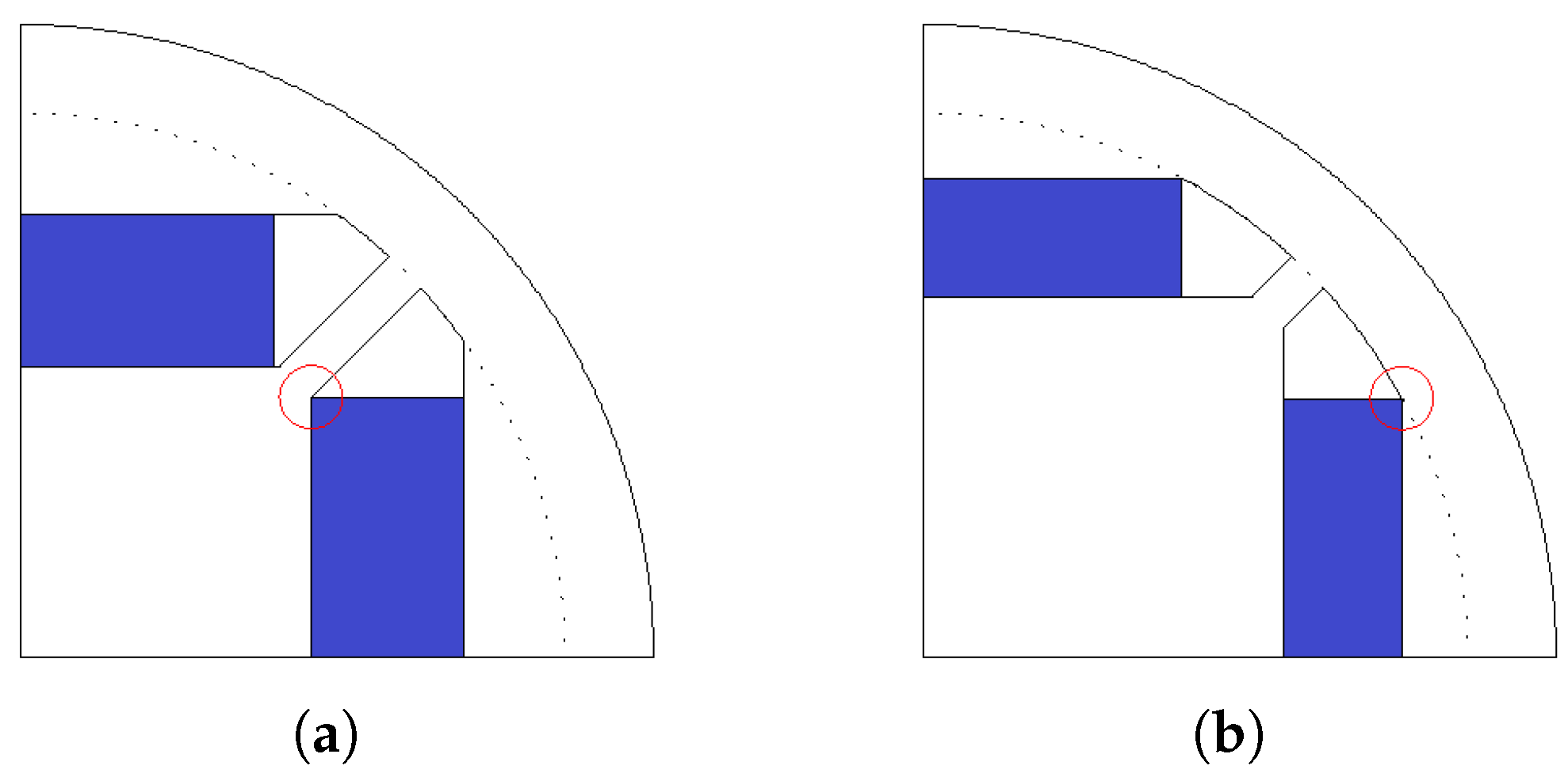
Figure 13.
Geometry conversion bug found in ANSYS Electronics Desktop. (a) ANSYS RMxprt geometry (PM thickness 4.58 mm); (b) generated ANSYS Maxwell model for (a); (c) ANSYS RMxprt geometry (PM thickness 4.59 mm); (d) generated ANSYS Maxwell model for (c).
Figure 13.
Geometry conversion bug found in ANSYS Electronics Desktop. (a) ANSYS RMxprt geometry (PM thickness 4.58 mm); (b) generated ANSYS Maxwell model for (a); (c) ANSYS RMxprt geometry (PM thickness 4.59 mm); (d) generated ANSYS Maxwell model for (c).
Figure 14.
Input and output parameters managed by solver class.
Figure 14.
Input and output parameters managed by solver class.
Figure 15.
Flowchart implementing the energy method (Rabbi et al.).
Figure 15.
Flowchart implementing the energy method (Rabbi et al.).
Figure 16.
Flowchart implementing the energy method (Chama et al.).
Figure 16.
Flowchart implementing the energy method (Chama et al.).
Figure 17.
Adapted flowchart implementing the eneryg method (Chama et al.).
Figure 17.
Adapted flowchart implementing the eneryg method (Chama et al.).
Figure 18.
Flowchartimplementing the time-domain method (Chama et al.).
Figure 18.
Flowchartimplementing the time-domain method (Chama et al.).
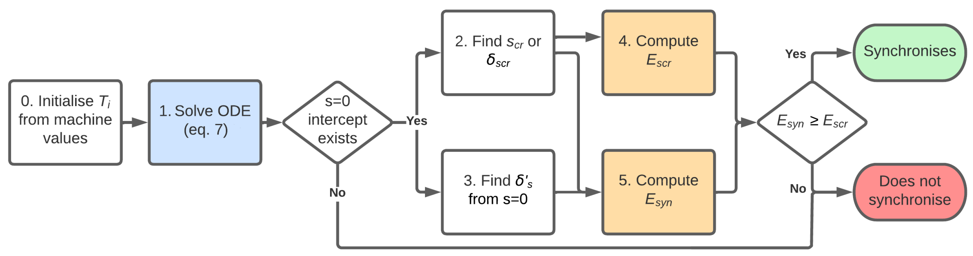
Figure 19.
Flowchart implementing binary search approach to determine .
Figure 19.
Flowchart implementing binary search approach to determine .
Figure 20.
Solver UI area adjusting by solver method: (a) solver area for the time-domain method (Chama et al.), (b) solver area for the energy method (Chama et al.).
Figure 20.
Solver UI area adjusting by solver method: (a) solver area for the time-domain method (Chama et al.), (b) solver area for the energy method (Chama et al.).
Figure 21.
Final GUI layout of analytical synchronization program.
Figure 21.
Final GUI layout of analytical synchronization program.
Figure 22.
Additional program features: (a) menu connecting to additional features and settings, (b) additional settings window.
Figure 22.
Additional program features: (a) menu connecting to additional features and settings, (b) additional settings window.
Figure 23.
The differential evolution process.
Figure 23.
The differential evolution process.
Figure 24.
Parameters to be varied during optimization: (a) available slot parameters, (b) available magnet parameters.
Figure 24.
Parameters to be varied during optimization: (a) available slot parameters, (b) available magnet parameters.
Figure 25.
Possible magnet width restrictions: (a) inner magnet width restriction, (b) outer magnet width restriction.
Figure 25.
Possible magnet width restrictions: (a) inner magnet width restriction, (b) outer magnet width restriction.
Figure 26.
Average population score per iteration.
Figure 26.
Average population score per iteration.
Figure 27.
Evolution of the power factor and critical inertia factor per iteration.
Figure 27.
Evolution of the power factor and critical inertia factor per iteration.
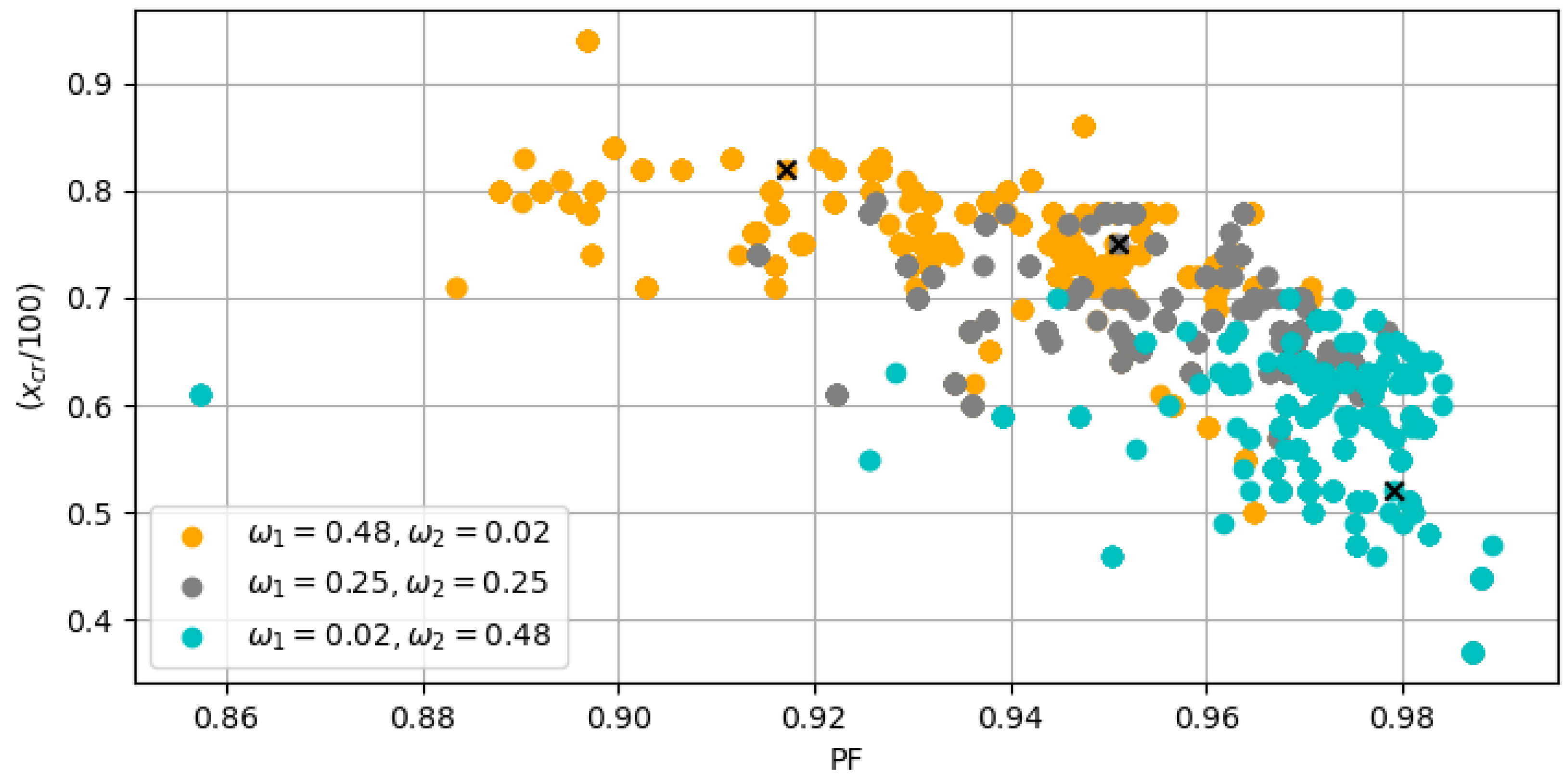
Figure 28.
Late DE iterations with varied weightings.
Figure 28.
Late DE iterations with varied weightings.
Figure 29.
Three designs chosen from the DE optimization results for comparison: (a) design 1, (b) design 2, (c) design 3.
Figure 29.
Three designs chosen from the DE optimization results for comparison: (a) design 1, (b) design 2, (c) design 3.
Table 1.
determined by various analytical methods for the machine set.
Table 1.
determined by various analytical methods for the machine set.
| | | Chama et al. (Time) | Chama et al. (Energy) | Rabbi et al. |
|---|
| Design | FEM | | | | | | |
| Radial 1 | 44 | 110 | 52 | 111 | 52 | 213 | 69 |
| Radial 2 | 40 | 112 | 49 | 113 | 50 | 225 | 67 |
| Radial 3 | 93 | 0 | 66 | 0 | 66 | 556 | 44 |
| V-Type 1 | 55 | 114 | 57 | 114 | 58 | 193 | 72 |
| V-Type 2 | 39 | 120 | 40 | 121 | 40 | 306 | 58 |
| V-Type 3 | 58 | 110 | 60 | 111 | 60 | 175 | 72 |
| W-Type 1 | 65 | 121 | 60 | 122 | 60 | 218 | 77 |
| W-Type 2 | 48 | 122 | 31 | 124 | 31 | 386 | 47 |
| W-Type 3 | 164 | 200 | 158 | 201 | 158 | 174 | 120 |
| Spoke 1 | 48 | 59 | 42 | 59 | 42 | 67 | 42 |
| Spoke 2 | 45 | 42 | 34 | 43 | 34 | 38 | 28 |
| Spoke 3 | 152 | 199 | 154 | 200 | 154 | 131 | 72 |
Table 2.
Computational time to determine test machine’s per method.
Table 2.
Computational time to determine test machine’s per method.
| Type of Method | Time (s) |
|---|
| Time-Domain Method (Chama et al.) | 33.667 |
| Energy Method (Chama et al.) | 450.852 |
| Energy Method (Rabbi et al.) | 0.500 |
Table 3.
determined by the energy method (Chama et al.) with various ODE solvers compared to target determined through FEM.
Table 3.
determined by the energy method (Chama et al.) with various ODE solvers compared to target determined through FEM.
| Type of LSPMSM | FEM | RK45 | Radau | BDF | LSODA |
|---|
| Radial 1 | 44 | 55 | 51 | 52 | 52 |
| Radial 2 | 40 | 53 | 49 | 50 | 49 |
| Radial 3 | 93 | 72 | 66 | 66 | 66 |
| V-Type 1 | 55 | 61 | 57 | 58 | 58 |
| V-Type 2 | 39 | 43 | 39 | 40 | 40 |
| V-Type 3 | 58 | 81 | 59 | 59 | 60 |
| W-Type 1 | 65 | 65 | 60 | 60 | 60 |
| W-Type 2 | 48 | 34 | 31 | 31 | 31 |
| W-Type 3 | 164 | 0 | 157 | 158 | 109 |
| Spoke 1 | 48 | 60 | 42 | 42 | 42 |
| Spoke 2 | 45 | 50 | 34 | 34 | 34 |
| Spoke 3 | 152 | 175 | 154 | 154 | 154 |
Table 4.
Computational time to determine using the energy method (Chama et al.) with different ODE solvers.
Table 4.
Computational time to determine using the energy method (Chama et al.) with different ODE solvers.
| ODE Method | Time (s) |
|---|
| RK45 | 402.086 |
| Radau | 550.320 |
| BDF | 450.852 |
| LSODA | 276.545 |
Table 5.
Approximate and Maxwell rotor inertias.
Table 5.
Approximate and Maxwell rotor inertias.
| Machine | Maxwell (kgm) | Approximated (kgm) | % Difference |
|---|
| Radial 1 | 0.0090446 | 0.0081215 | 10.21 |
| Radial 2 | 0.0090446 | 0.0081178 | 10.25 |
| Radial 3 | 0.0090446 | 0.007938 | 12.23 |
| V-Type 1 | 0.0090446 | 0.0081899 | 9.45 |
| V-Type 2 | 0.0090446 | 0.0082991 | 8.24 |
| V-Type 3 | 0.0090446 | 0.0081992 | 9.35 |
| W-Type 1 | 0.0090446 | 0.0080894 | 10.56 |
| W-Type 2 | 0.0090446 | 0.0082279 | 9.03 |
| W-Type 3 | 0.0090446 | 0.0077131 | 14.72 |
| Spoke 1 | 0.0090446 | 0.0083418 | 7.77 |
| Spoke 2 | 0.0090446 | 0.0083635 | 7.53 |
| Spoke 3 | 0.0090446 | 0.0077431 | 14.39 |
Table 6.
Comparing Go and Python ODE solvers for predicting .
Table 6.
Comparing Go and Python ODE solvers for predicting .
| Machine | Python LSODA | Go RK45 |
|---|
| Radial 1 | 52 | 51 |
| Radial 2 | 49 | 49 |
| Radial 3 | 66 | 61 |
| V-Type 1 | 57 | 57 |
| V-Type 2 | 40 | 39 |
| V-Type 3 | 60 | 59 |
| W-Type 1 | 60 | 60 |
| W-Type 2 | 31 | 31 |
| W-Type 3 | 158 | 108 |
| Spoke 1 | 42 | 42 |
| Spoke 2 | 34 | 34 |
| Spoke 3 | 154 | 120 |
Table 7.
Restrictions for magnet dimensional parameters.
Table 7.
Restrictions for magnet dimensional parameters.
| Parameters | Minimum | Maximum |
|---|
| 1. D1 | 2 | 2( − slot depth − CDG) |
| 2. O1 | | D1/2 |
| 3. MagT | > 0 | D1/2 − O1 |
| 4. Rib | | |
| 5. MagW | > 0 | Equation (22) |
Table 8.
Critical inertia factors, lifetimes, and scores of DE designs.
Table 8.
Critical inertia factors, lifetimes, and scores of DE designs.
| | Analytical | FEM | | | PF | (kW) |
|---|
| Design 1 | 63 | 43 | 0.02 | 0.48 | 0.979 | 2.2 |
| Desing 2 | 75 | 55 | 0.25 | 0.25 | 0.951 | 2.2 |
| Design 3 | 82 | 57 | 0.48 | 0.02 | 0.917 | 2.2 |


