Optimal Scheduling of Neural Network-Based Estimated Renewable Energy Nanogrid

Abstract

In developing countries, many areas are deprived of electrical energy. Access to cleaner, more affordable energy is critical for improving the poor’s living conditions in developing countries. With the advent of smart grid technology, the integration and coordination of small grids, known as nanogrids, has become very easy. The purpose of this research is to propose a nanogrid model that will serve the purpose of providing the facility of electrical power to the poor rural community in Pakistan using hybrid renewable energy sources. This paper targets the electrification of a poor rural community of Akora Khatak, a small district located in Pakistan. The mathematical modeling of solar and wind energy, neural network-based forecasting of solar irradiance and wind velocity, and the social analysis to calculate the payback period for the community have been discussed in this paper.

1. Introduction

The world population is increasing day by day, thus demanding more and more electrical energy for their needs according to [1]. The power obtained from the conventional resources of energy no longer remains enough in this modern age. Furthermore, according to [2], the harmful effects of the pollutants emanating from these resources have always urged researchers to find alternative resources of energy. This energy deficiency can easily be met by using renewable energy resources without any adverse environmental effects. Renewable energy resources are environment-friendly, easily available, and cost-effective according to references [3,4]. In various parts of the world, there are many areas where electrification has not been done yet. These types of areas are usually located very far from the load centers, making it difficult to supply power. The best solution to this problem is to develop a small nanogrid for such a community using renewable energy resources. Currently, many scientists are working on such types of electrification projects in distant areas as stated in references [5,6]. The model includes the optimization of solar, wind, and battery energy storage systems. A combination of renewable energy resources forms a very complex engineering problem that needs to be optimized accurately to find the minimum cost of the system. One such example is demonstrated in this research, wherein a multivariate and complex system is optimized using the convex optimization algorithm to find the minimum cost of the system installed in a poor distant rural community.

Many researchers have worked on power availability in rural areas and proposed solutions. Previously, the researchers proposed a model based on natural resources [7], including coal, oil, and natural gas for poor rural areas, but the overall cost and harmful emissions were very large. However, nanogrids that are integrated from renewable energy resources due to their lower cost and environment-friendly nature prove to be more effective for the poor rural areas where electricity is unavailable according to [8]. Some researchers mentioned in [9] have taken into consideration the grid power in addition to renewable energy, while some have proposed a solution with grid-independent renewable energy sources as mentioned in [10,11,12]. In the past, a system comprising renewable energy resources using one or more types of sources came out to be the most effective solution for the electrification of these under-developed poor rural areas. In these types of systems, the solar and wind combination is the most stable and reliable system due to its low cost, ease of availability, and minimum outage time. Further, battery energy storage systems (BESS) are also being used to ensure energy availability during nighttime and to make the system reliable. According to reference [13], researchers have worked on the electrification of a poor rural area named “Kadayam” located in Tamilnadu, India. In the analysis, it was shown that the combination of wind and solar is the best feasible solution for the electrification of the community. It is further investigated that enhancing the nearby existing grid is not the recommended solution due to its harmful effects on the environment and high cost. In the end, it was concluded that the combination of solar, wind, and hydro generation could meet all the load demands of the community throughout the day without any fluctuations and loss of supply. Hence, it is the most reliable and cost-effective solution to the problem. Similarly, according to reference [14], another person has worked in this area for the sake of electrification of poor rural areas in the country. The feasibility of the system in a small rural community Urumqi located in China was studied in detail. From the analysis, it was concluded that the combination of PV, wind, and battery energy storage systems is the cost-effective and reliable solution to the energy shortage. For this purpose, the optimization techniques were applied to the system and it was revealed that for the lowest cost of the system, 72% of the energy should be taken from the solar and 28% of the energy should be taken from the wind source. It was also noticed that with any further increase in energy demand in that area, an increase in solar percentage rather than wind is a more efficient solution from the cost point of view. The concept of the establishment of a nanogrid and its topologies has been presented in [15], vide which nanogrids can be established in many countries. One another very good manifestation of setting up the nanogrid by producing electrical energy from renewable energy resources is presented in [16], in which a master controller has been used for the energy mix of various renewable energy resources. This paper also focuses on establishing the nanogrid for the poor rural community using advanced forecasting techniques of neural networks.

2. Methodology

To solve the optimal dispatch problem, a very accurate and robust programming technique should be applied to the proposed problem. As seen from the literature [17], the objective function of the proposed problem involves the linear combination of powers corresponding to various renewable energy resources. This forms a multi-variable convex optimization problem whose global optima exist at a specific point. Hence, for this type of problem, the results obtained from the convex optimization algorithms have been seen to be more accurate as compared to probabilistic algorithms, according to the references [18,19]. For the same reason, convex optimization has been implemented in this research.

3. Research Gap and Contributions

The following objectives have been obtained from the proposed research:

(a)

To propose a grid-independent efficient small nanogrid model of a hybrid renewable energy resource system for a poor rural area located in Pakistan.

(b)

To design a Bayesian regularization-based neural network model for data forecasting.

(c)

To optimize the power-sharing between renewable energy sources by using an efficient algorithm.

(d)

To find the minimized cost of the nanogrid to make the model economical.

(e)

To implement the electrification of poor rural areas of Pakistan using this efficient optimal scheduling.

(f)

To perform the social analysis for the poor rural community and calculate the payback period.

4. Proposed System Architecture

The system under consideration consists of solar, wind, and battery energy storage system to meet the load demand of the community. Figure 1 shows the pictorial representation of the architecture of the proposed system containing various renewable energy resources. The problem will be solved for complete one day. During each hour, the load demand is different, which means that the load is dynamic, so the optimization problem is scheduled for every hour. During optimization, the various constraints are also kept active. For solar energy, these constraints include the power limits available each hour according to the irradiance level. Similarly, for wind energy, there is also a limit on maximum and minimum power available depending upon the wind speed in that interval. These constraints are used actively along with the highly complex multivariable objective function. The function is a cost function, and hence it needs to be minimized. This problem is called the convex cost minimization problem.

5. Solar Energy System

5.1. Electrical Modeling of Solar Cell

In the optimization problem under consideration, there is a need for a very accurate model to calculate the output power of a solar cell [20]. The power output of a solar cell is a function of solar irradiance and temperature. There are many models available that have been used extensively in the past. One such model given by [21] has been used here due to its accuracy and versatility. This model has been derived using fractional and integral polynomials and thus making it very accurate and sensitive to the change in solar irradiance and temperature. In this mathematical model, the voltage-current characteristics have been approximated by the polynomial expansion method. The final result demonstrates the output current of a solar cell as a function of the operating voltage. The output power of one solar cell can then be easily calculated by the product of operating voltage and output current. The output current of a solar cell as a function of operating voltage is given by Equation (1).

$$I\left(V\right)=I_{s.c}-I_{s.c}{\left(\frac{V}{V_{o.c}}\right)}^{a+b}$$

(1)

where $I_{s.c}$ is the solar cell short circuit current, I is the output current of the solar cell and it will be bounded between 0 and $I_{s.c}$, V is the output voltage of the solar cell, and it will be bounded between 0 and $V_{o.c}$, a is a positive integer, b is a non-negative integer between 0 and 1, a + b is the sum which depends upon the values of nominal and short circuit current and $P_o$ is the power of the solar cell as a function of voltage and current.

The power extracted from the solar cell can be calculated by the product of operating voltage and current as a function of current. The expression for the power is given by Equation (2):

$$P\left(V\right)=I\left(V\right)V$$

(2)

Now, putting the value of $I\left(V\right)$ from Equation (1) into Equation (2):

$$P\left(V\right)=\left(I_{s.c}-I_{s.c}{\left(\frac{V}{V_{o.c}}\right)}^{a+b}\right)V$$

(3)

It can be seen through Equation (1) that to calculate the output current of the solar cell in terms of operating voltage, various parameters are needed. These include the short circuit current and open circuit voltage of a solar cell plus the integers a and b. These parameters can be easily calculated from Equations (4)–(6).

$$V_{o.c}=s_i\frac{E_i}{E_{in}}TCV\left(T-T_n\right)+s_i{V}_{max}-s_i\left(V_{max}-V_{min}\right)s_i\times \exp \left(\frac{E_i}{E_{in}}\times \ln \left(\frac{V_{max}–V_{o.c}}{V_{max}-V_{min}}\right)\right)$$

(4)

$$I_{s.c}=p_i\frac{E_i}{E_{in}}\left(I_{s.c}+TCI\left(T-T_n\right)\right)$$

(5)

$$a+b=\frac{I_{s.c}}{I_{s.c}-I_{op}}$$

(6)

where $s_i$ is the total number of solar cells added in series, $p_i$ is the total number of solar cells added in parallel, $E_i$ is the effective solar irradiance level, $E_{\mathit{in}}$ is the solar irradiance level at standard temperature and pressure, T is the current temperature value given at that particular instant, $T_n$ is the temperature at standard conditions, $V_{min}$ is the minimum value of solar cell voltage, $V_{max}$ is the maximum value of solar cell voltage, $V_{op}$ is the nominal operating voltage of the solar cell, $I_{op}$ is the nominal operating current of the solar cell, TCV is the temperature coefficient for open circuit voltage and TCI is the Temperature Coefficient for short circuit current.

It is important to note that values of open circuit voltage and short circuit current only need to be updated when the solar cell is operating at some conditions other than the standard ones. At standard operating conditions, the nominal rated values of voltage and current of the solar cell directly give the open circuit voltage and short circuit current limits, and no calculations are required at all.

The standard parameters of the solar cell model used in this research are listed below in the form of

Table 1. Standard parameters of the solar cell model.

Variable Name	Value
$V_{o.c}$	21.6 $\mathrm{V}$
$I_{s.c}$	4.8 $\mathrm{A}$
$V_{max}$	22 $\mathrm{V}$
$V_{min}$	18 $\mathrm{V}$
$V_{op}$	17.1 $\mathrm{V}$
$I_{op}$	4.3 $\mathrm{A}$
$E_{in}$	1000 $\frac{\mathrm{W}}{{\mathrm{m}}^2}$
$T_n$	$25{}^{\circ }\mathrm{C}$
$TCV$	−0.076 V/°C
$TCI$	0.00205 V/°C

.

5.2. Programming of Model in MATLAB

Once the model is finalized with all the parameters, the next step is the implementation of this model in MATLAB (R2018a) for detailed analysis. It is because of the reason that the model equations depend upon various parameters such as temperature and irradiance plus the integers a and b. So, it is necessary to validate the model against all the parameters. This is done by passing these parameters first independently one by one and then collectively at one time in the mathematical model. Using the mathematical equations of this solar cell model, a very accurate and versatile code has been written in MATLAB. The flowchart or the pseudo-code for the model is shown in Figure 2.

6. Wind Energy System

6.1. Electrical Modeling of Wind Energy

After successful modeling of the solar cell, the second most important thing required for the optimization problem under consideration is the power output available from the wind turbine. The power output from the wind energy system has been extensively used in the past as a source of renewable energy, according to references [22,23]. With the increase in the population of the world, all the energy demands cannot be met by conventional sources of energy. To compensate for this deficiency, wind power is also employed in conjunction with solar energy. The power output from the wind system varies with different parameters, such as the density of the air and the area of rotor blades, but it varies more significantly as a function of wind velocity. The word “significant” should be used here because it varies as the cubic function with the wind velocity. In large coastal areas, many wind plants are connected in concatenation to produce bulk useful power at the output. The output power from the wind energy system is a function of air density, blades area, and wind velocity and is given by Equation (7):

$$P_w=\frac{1}{2}·\rho A·{\left(v_w\right)}^3$$

(7)

Here $P_w$ is the power extracted from the wind source in (W), ρ is the density of air in (Kg/m³), A is the area of blades of a rotor in (m²), and $v_w$ is the speed of wind in (m/s).

6.2. Programming of Model in MATLAB

After the detailed theoretical analysis and investigation of various dependent parameters of the wind energy conversion system, the power extracted by the wind energy system is programmed in MATLAB for further analysis. The validation of the model is very important because there are so many dependent parameters that need special attention for studying their effects. Using the wind energy system equations and their various parameters, a very versatile and accurate program is written in MATLAB, which calculates the power output for a given set of input parameters. The flowchart or the pseudo-code for the model is shown in Figure 3.

7. Forecasting Using Neural Networks

7.1. Time Series Forecasting Analysis

A time series plot is the graph of a particular data set over a specific period of time. Time series analysis has been extensively performed in the past for predicting future values [24]. The process is called time series forecasting analysis. In this analysis, the values for a particular variable are predicted depending on the dataset available from the past. Many forecasting techniques have been used commonly in the past. Each technique has its specialty, advantages, and disadvantages. A large-scale comparison between the traditional logistic regression and neural networks has been exhibited in [25], vide which a comparison

Table 2. Neural network and logistic regression comparison by attributes.

Sr. No.	Attribute	Neural Network	Logistic Regression
1	Accuracy	Good	Fair
2	Complex Interactions	Good	Poor
3	Interpretation of Weights	Fair	Good

is shown below.

Keeping in view the complexity of the problem, the large dataset, and the good attributes, it is clear that one should choose neural networks rather than traditional logistic regression. Hence, a neural network algorithm has been used in this research.

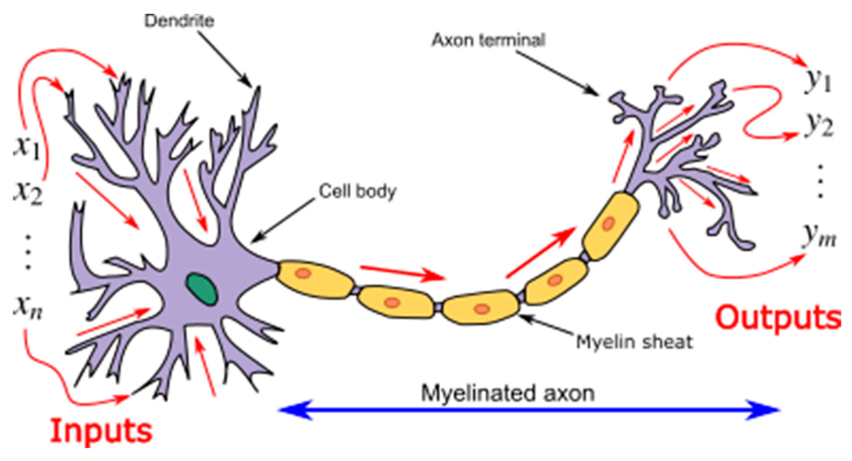
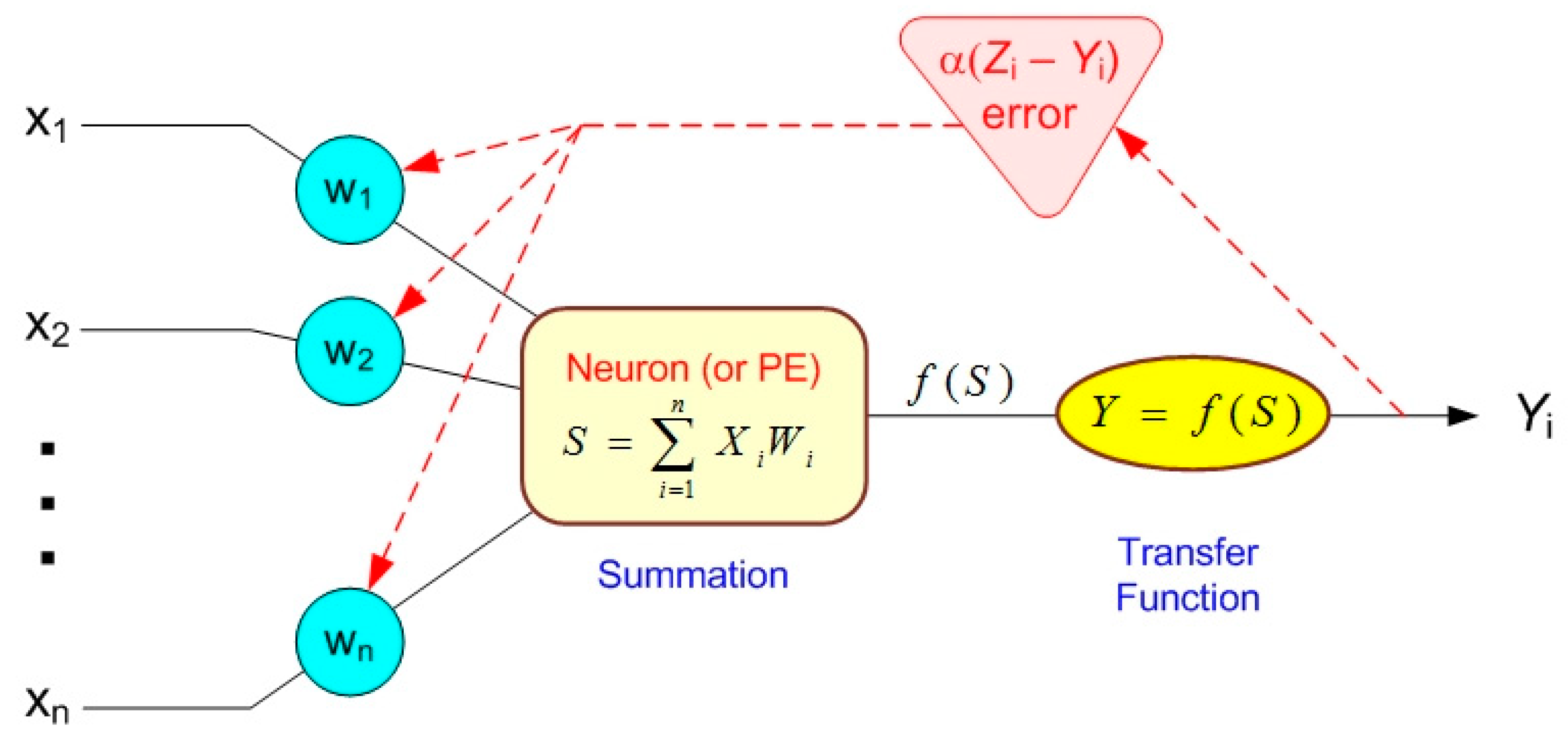
A neural network-based technique that involves highly intelligent neurons, just like human ones, to predict future values has been implemented here [26,27]. To demonstrate the forecasting analysis, suppose there exist a series of data having dependence on time t given by Equation (8):

$$V\left(t\right)=\left[x\left(t_0\right),x\left(t_1\right),x\left(t_2\right),\dots .,x\left(t_i\right)\right]$$

(8)

Here V(t) is the vector containing the values of variable x at different time instances, and x($t_i$) represents the magnitude of variable x at time instant i.

Using the previous values of the variable x from the past as given in the vector V(t), the desired value can be predicted by using a particular function f and is given by Equation (9).

$$x\left[t+p\right]=f\left(x\left(t_0\right),x\left(t_1\right),x\left(t_2\right),\dots .,x\left(t_i\right)\right)$$

(9)

Here $x\left[t+p\right]$ is the predicted value of the variable x at some time instant $t+p$ which is often called the length of prediction.

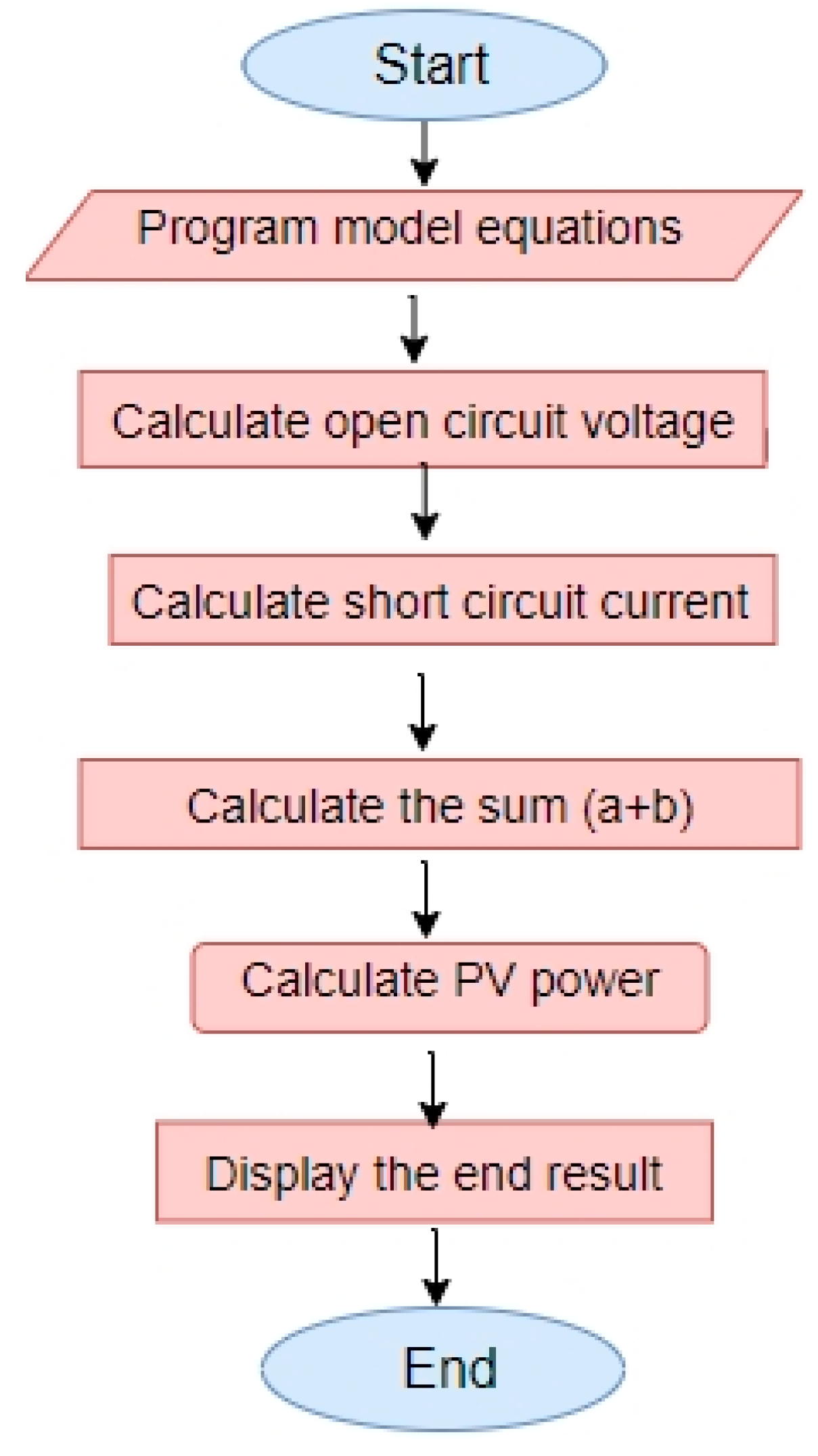
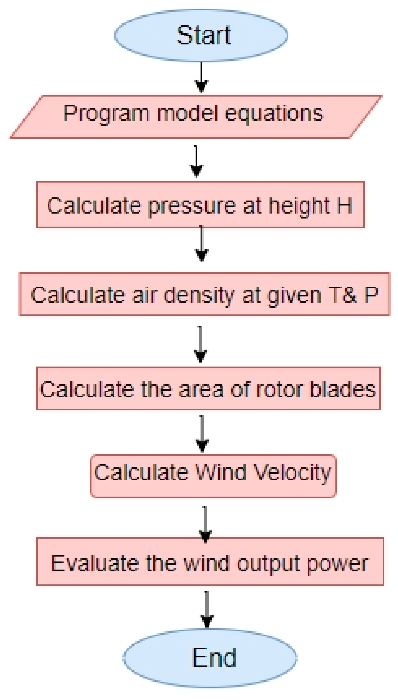
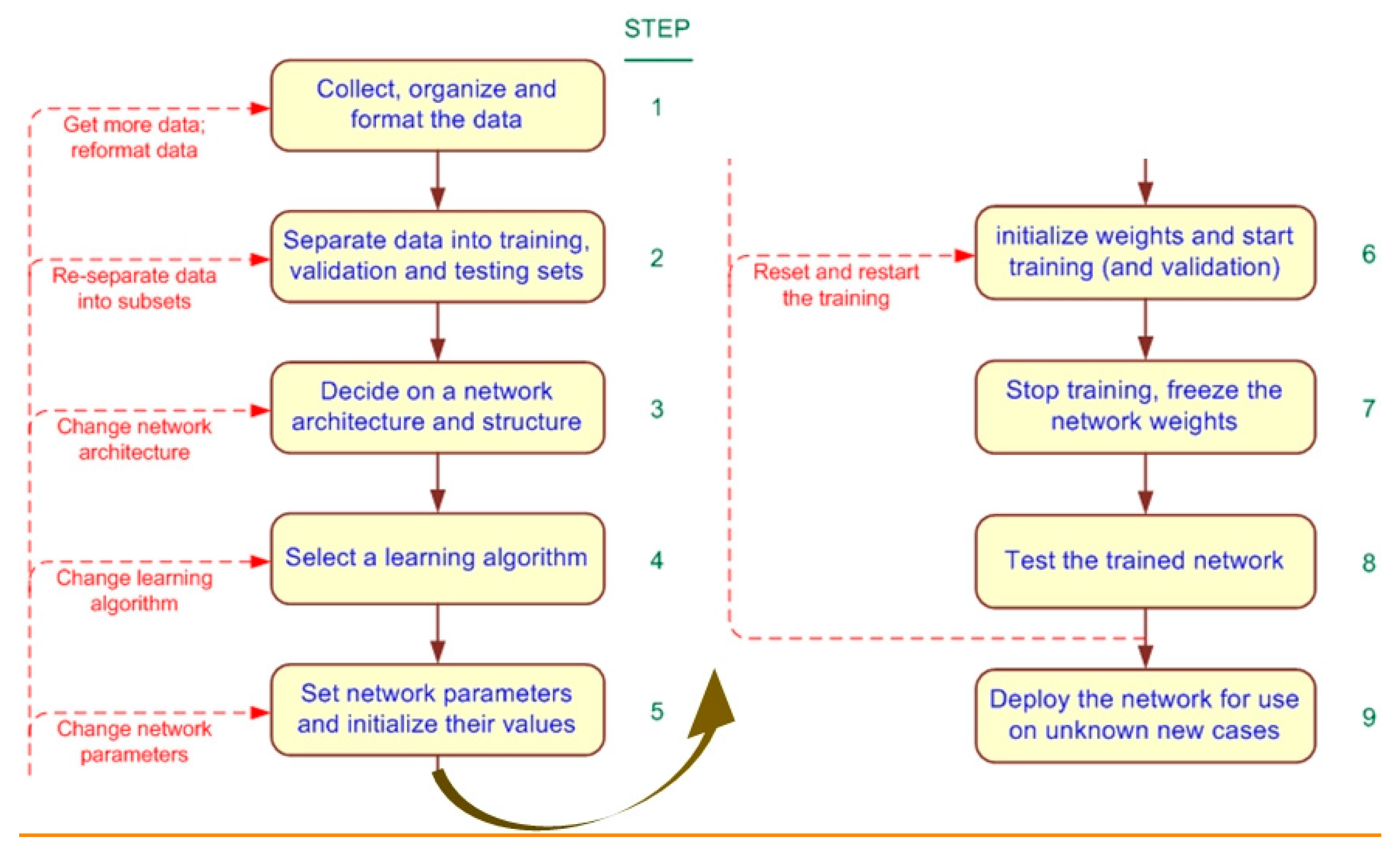
The following problem can be easily solved by approximating the function which is closest to the model and thus gives a minimum mean square error. The process involves the following steps:

(a)

Choose the appropriate algorithm.

(b)

Train the network for every value of a variable at various time instances $t_i$.

(c)

Calculate the mean square error and adjust the weights.

(d)

In the end, just evaluate the model at the desired time instant $t+p$.

7.2. Neural Networks

An Artificial neural network is a very complex set of computing algorithms designed by considering the same topology exhibited by the human brain [28,29,30]. Although one cannot reach the complexity equal to the human brain, a very finely tuned algorithm can be built by using the human brain’s working methodology. The network consists of many neurons, also called nodes. Each node carries a distinct state which is calculated by the weighted sum of the input values to the network. The weight assigned to the neuron gives the strength of that neuron signal. For example, a signal with high signal strength will be considered as logic 1 and will transfer the data to the next layer as compared to a neuron that has low strength and hence will be discarded. The weights associated with each neuron are not constant, rather, they keep on updating for fine-tuning of the network. The output signal of each neuron cell is determined by the weighted sum of inputs and is often known as the activation function. A very basic functional diagram of human neurons is shown in Figure 4.

The above figure represents the signal flow diagram of a human brain. The system has the inputs in the form of some sense signal. The signal thus flows through the information-carrying input processing cells called dendrites. The signal then flows through the main layers of the neural system called the myelinated axon. The output stage consists of other information-carrying cells called Axon terminals. The information signal is decoded here and output in the form of some pain or happiness is observed by the human being.

A very similar approach is used in designing the artificial neural network and is shown in Figure 5.

In the above figure, there is a set of input layers followed by a hidden layer. The number of hidden layers shows the complexity of the neural network and directly affects the learning rate of the system. The final stage consists of a set of the output layer. Each connection is assigned a specific weight and is used to calculate the signal strength of each neuron.

7.3. Neural Network Training Using Backpropagation

One of the best training techniques that are often used to train the neural network is the backpropagation method [33,34]. In this type of method, the error obtained after every propagation is fed back towards the input to reduce its magnitude in each cycle. This is a highly effective method, as the mean square continuously reduces after every cycle. The block diagram for the backpropagation of the neural network system is given in Figure 6.

In the above figure, it is clear that the error generated at the output of the process is propagated back to the input side, thus reducing the error magnitude very quickly.

The backpropagation methodology involves the following steps:

(a)

Assign values to the weights and start the process.

(b)

Pass the inputs and true values at the output.

(c)

Evaluate the output of the neural network.

(d)

Calculate the error by taking the difference between the actual output and the true value.

(e)

Evaluate the output of the neural network.

(f)

Update the various weights associated with the network by propagating the error backward.

(g)

Repeat the above procedure many times till the weights are adjusted according to the required output and error is minimized.

The data set is split into three parts, i.e., training, validation, and testing. Very often, almost 70 percent of the data is taken for training and the other 30 percent is distributed in validation and testing. A pseudo-code or flowchart of training of the neural network using the backpropagation technique is shown in Figure 7.

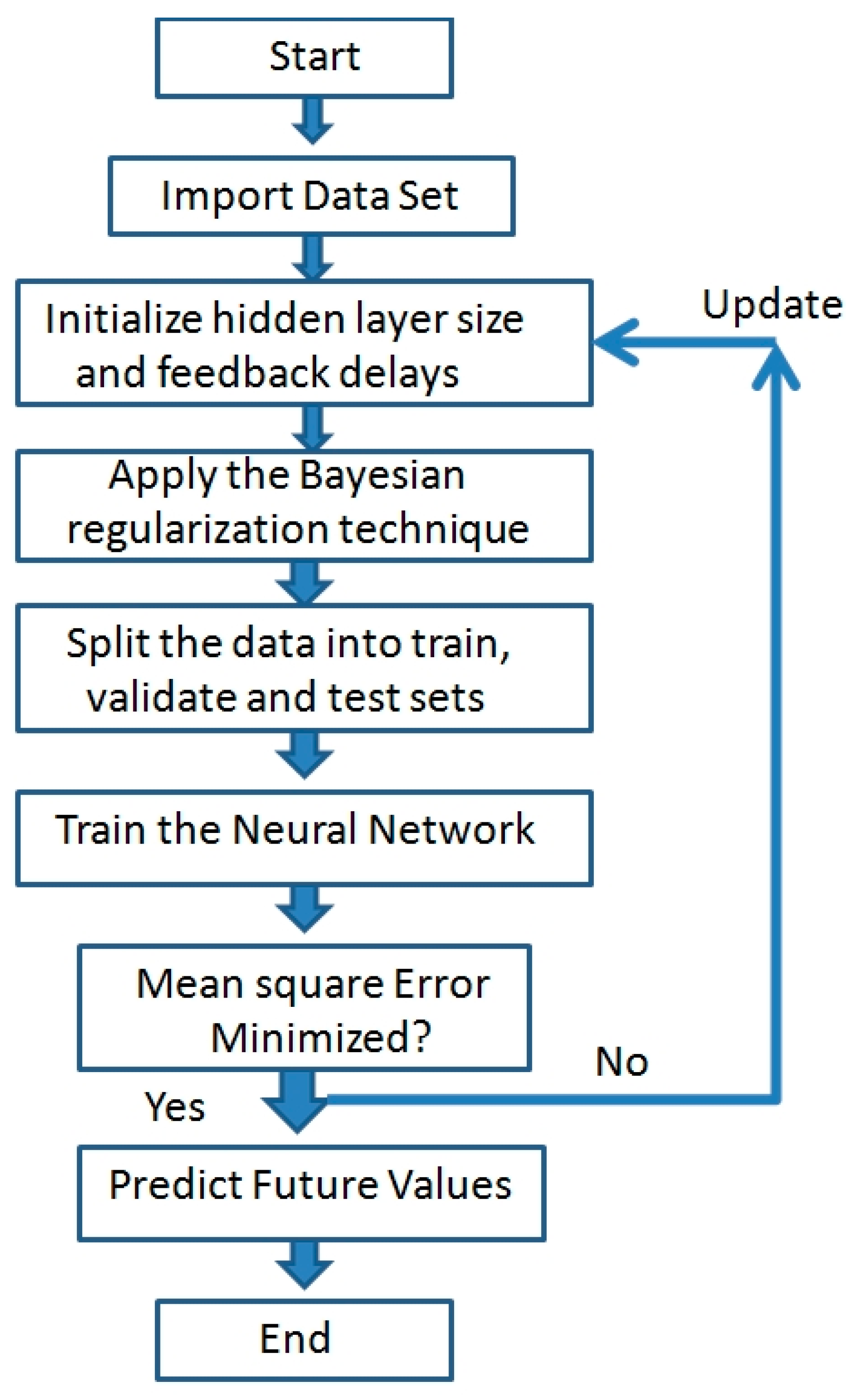
7.4. Bayesian Regularization-Based Back Propagation Neural Networks

In the implementation of the backpropagation methodology, there must be a suitable and effective function that will propagate the error backward in such a way that the probability of the mean square error increases and accurate results can be obtained. There are many algorithms that have been used in the past, but the most accurate and versatile algorithm is the Bayesian regularization algorithm. Other such types of algorithms may include Levenberg Marquardt (also known as the LM algorithm). However, it has been observed that Bayesian regularization gives the maximum probability of fitting the data set as compared to the LM algorithm, thus reducing the chance of overfitting the system. Further, it is also observed that Bayesian regularization algorithms provide the highest level of correlation coefficients and the least amount of mean square error [36]. As a result, this algorithm gives the result with the highest level of accuracy and consistency. This is the same reason why this algorithm has been used in this research.

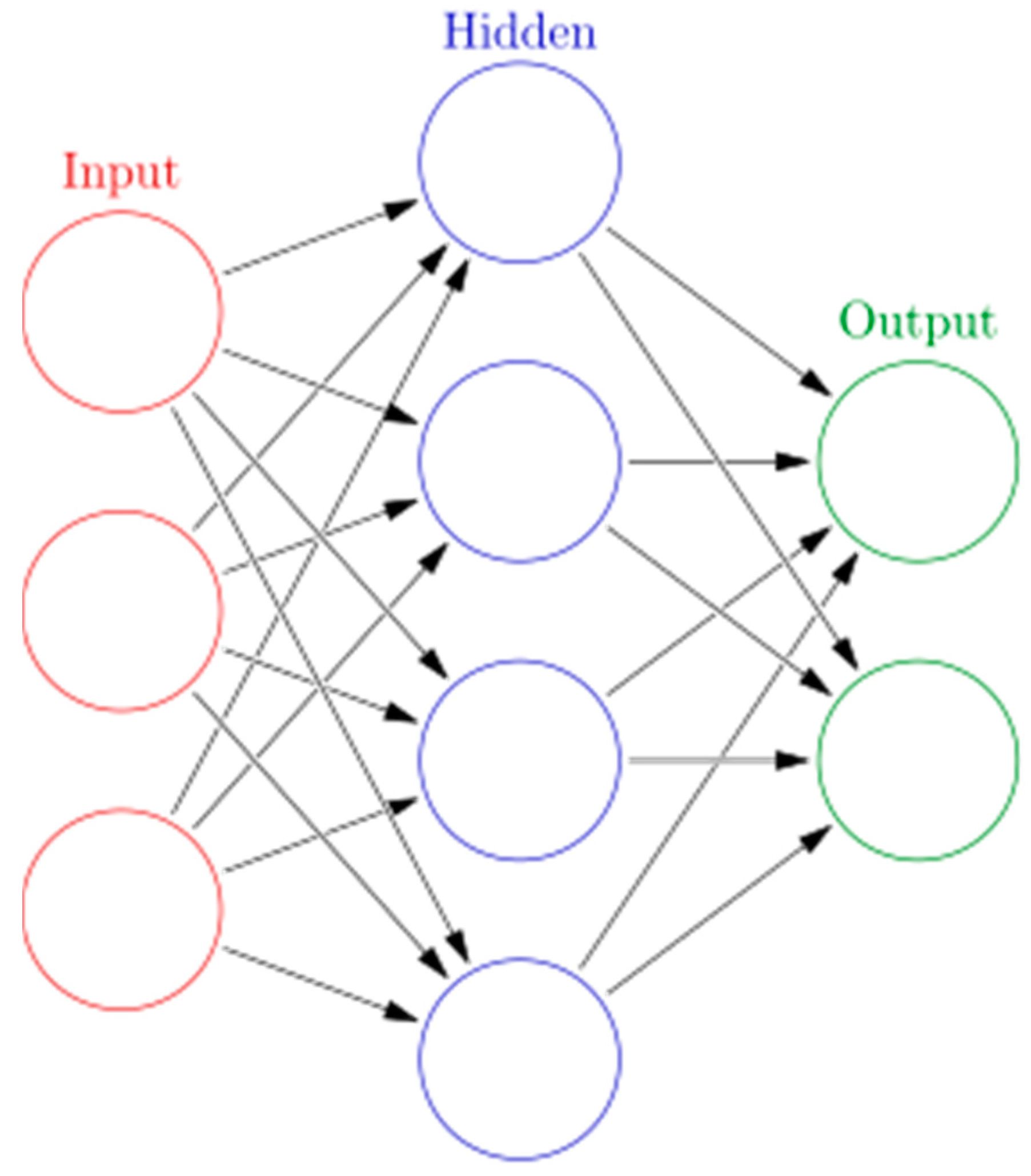
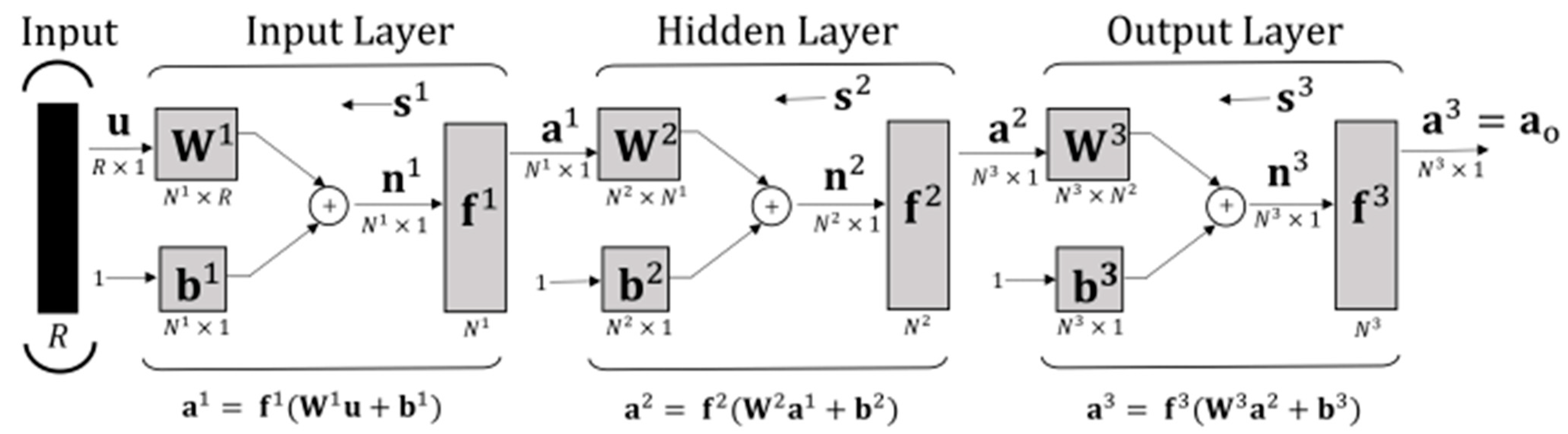
To show the methodology of the algorithm, suppose a neural network system consisting of input layer $L_i$, hidden layer $L_h$ and output layer $L_o$. The input to the system is represented by $U_i$ is associated with the input weight matrix $W_1$ and a bias term $b^1$ to yield the output of first layer $a_1$ which acts as the input to the activation function $f^1$. The effective output of the first layer is then given by the activation function $f^1$. The bias is added to increase the flexibility of the overall system. The output of the first layer $a_1$ acts as an input to the hidden layer $L_h$, interacts with the Weight matrix $W_2$ and bias term $b^2$ to activate the transfer function $f^2$ for an output of $a_2$. Lastly, $a_2$ is given to the output layer as an input which combines the effect of a weight matrix $w_3$ and bias term $b^3$ to give a signal to the activation function $f^3$, which then calculates the final output $a_3$ of the system. In general, a neural network consisting of $N_1$ no of layers, weight matrix $W_1$ and bias vector of $b^1$ for any given layer l can be modeled in the form of Equation (10).

$$W^l=\left[\begin{array}{cccc}{w}_{11}^l& w_{12}^l& \dots & w_{1R}^l\\ w_{21}^l& w_{22}^l& \dots & w_{2R}^l\\ ⋮& ⋮& \ddots & ⋮\\ w_{N1}^l& w_{N2}^l& \dots & w_{NR}^l\end{array}\right],b^l=\left[\begin{array}{c}{b}_1^l\\ b_2^l\\ ⋮\\ b_N^l\end{array}\right]$$

(10)

Here $n^1$ represents the total number of processing cells in the particular layer l. The magnitude of the signal at the input side of the activation function is given by Equations (11) and (12):

$$n^l=W_l{a}_{l-1}+b^l$$

(11)

and

$$a^0=input$$

(12)

Here, $N^1$ shows the total amount of neurons in layer $n^1$, $N^2$ shows the total amount of neurons in layer $n^2$ and $N^3$ shows the total amount of neurons in layer $n^3$. The number of neurons of the first and last layer is directly associated with the input and output layers. In contrast, the inner layers’ neurons help in adjusting the weights while keeping in view the condition of least mean square error. A back propagation neural network consisting of input, hidden, and output layers is shown in Figure 8.

The network error is evaluated at the end of each iteration by taking the difference between the calculated value $a^0$ and exact value $t_o$. This error is then backpropagated to update the values of weights associated with various neurons. Very often, the error in a layer is given by the weighted sum of the sensitivity. Here, the term sensitivity of the neural network means the change in the output with the variation in the input values. There are a number of algorithms that are used in the literature to give the relation between the sensitivity and error of any layer l of the neural network. One such relation known as the recurrence relation, is given by Equations (13) and (14).

$$s^l={\dot{F}}^l\left(n^l\right)W^{l+1}{s}^{l+1}$$

(13)

and

$$s^{nl}={\dot{F}}^{nl}\left(n^{nl}\right)\left(t_o-a_o\right)$$

(14)

Here,

$$l=n-1,n-2,\dots ,3,2,1$$

Here $F^1$ is a matrix that is diagonal and it contains the partial derivatives of the transfer function $f^l$ with respect to the variable $n^l$. The matrix is given by Equation (15):

$${\dot{F}}^l\left(n^l\right)=\left[\begin{array}{cccc}{\dot{f}}^l\left(n_1^l\right)& 0& \dots & 0\\ 0& {\dot{f}}^l\left(n_2^l\right)& \dots & 0\\ ⋮& ⋮& \ddots & ⋮\\ 0& 0& \dots & {\dot{f}}^l\left(n_N^l\right)\end{array}\right]$$

(15)

In some cases, when the transfer function chosen is a linear one, the above matrix will be a unit or identity matrix.

It is important to note here that the reverse propagation of error updates the weights of the hidden layer to obtain the best results at the output. Now, if the data is processed backward too many times, the model will become hard familiar with only the current data set. This may lead to overfitting of the model, which needs to be avoided. It is because the overfitted model may give the least amount of mean square error but with the compromise of loss of sensitivity. Hence, it will perform poorly when a new data set is passed through the model. Therefore, a good model should give the minimum amount of error, and it should work well with new data sets as well.

To compute the mean square error of the model, consider a data set d consisting of input vector v and output true values t. The data vectors in terms of input-output order pairs are given by Equation (16).

$$d=\left[\left(v_0,t_0\right),\left(v_1,t_1\right),\dots .,\left(v_n,t_n\right)\right]$$

(16)

Now, the output against each input obtained deviates from the true known values, thus generating an error for the first-order pair. Similarly, the error in the ordered pair of the data set is generated for the complete size of the data array. The error thus computed is represented in the form of a performance index which is a term used for the direct measurement of how much the model is accurate and robust. The overall performance index of the neural network model is given by Equations (17) and (18):

$$F\left(\overline{w}\right)={\sum }_{j=1}^n{(e_j)}^2={\sum }_{j=1}^n{(t_{0j}-a_{0j})}^T\left(t_{0j}-a_{0j}\right)$$

(17)

and,

$${(\overline{w})}^T={[w^1,w^1,\dots .,w^n]}_{1\times K}$$

(18)

Here, ${(\overline{w})}^T$ is the weight vector of size K containing all the weights.

With,

$$K=N^1\left(R+1\right)+N^2\left(N^1+1\right)+\dots +N^n\left(N^{n-1}+1\right)$$

To make the model robust, the above neural network model can also be expressed in a more general form by adding a penalty factor term in the performance index relation. The new relation after the addition of (μ/ν)$E_w$ as a penalty term is given by Equation (19).

$$F\left(\overline{w}\right)=\mu E_w+\nu E_D$$

(19)

Here, μ and ν represent the Bayesian regularization parameters while $E_w$ represents the whole network mean square error. The $E_w$ (NMSE) is given by Equation (20)

$$E_w={(\overline{w})}^T\left(\overline{w}\right)$$

(20)

Now, the main objective in training the neural network is the calculation of the Bayesian regularization parameters, i.e., μ and ν. If μ < ν, the error calculated will be too smaller that it can be ignored. On the other hand, if μ > ν, then the error will be considerable and it cannot be ignored. To find the optimal values of μ and ν in a given data set, consider the weight vector $\overline{w}$ as a random variable with the objective of finding the maximum probability $P\left(\overline{w}|d,\mu ,\nu ,M_n\right)$ of the weight which minimizes the mean square error. This probability can be calculated by using the Bayes rule, which states that the expression can be written in terms of probability function $P\left(d|\overline{w},\nu ,M_n\right)$, prior density $P\left(\overline{w}|\mu ,M_n\right)$ and the normalization factor $P\left(d|\mu ,\nu ,M_n\right)$. The expression is given by Equation (21):

$$P\left(\overline{w}|d,\mu ,\nu ,M_n\right)=\frac{P\left(d|\overline{w},\nu ,M_n\right)\times P\left(\overline{w}|\mu ,M_n\right)}{P\left(d|\mu ,\nu ,M_n\right)}$$

(21)

Assuming the error in the data set has the Gaussian distribution, the probability function takes the form of Equation (22):

$$P\left(d|\overline{w},\nu ,M_n\right)=\frac{\exp \left(-\nu E_D\right)}{Z_D\left(\nu \right)}$$

(22)

With,

$$Z_D\left(\nu \right)={(\pi /\nu )}^{\frac{Q}{2}},Q=n\times N^l$$

Likewise, prior density can be written in the same manner by considering the weights as the Gaussian distribution. The prior density $P\left(\overline{w}|\mu ,M_n\right)$ will be calculated by using Equation (23):

$$P\left(\overline{w}|\mu ,M_n\right)=\frac{\exp \left(-\mu E_w\right)}{Z_w\left(\mu \right)}$$

(23)

With $Z_w\left(\mu \right)={(\pi /\alpha )}^{\frac{K}{2}}$

Hence, the probability $P\left(\overline{w}|d,\mu ,\nu ,M_n\right)$ can be written in the form of Equation (24):

$$P\left(\overline{w}|d,\mu ,\nu ,M_n\right)=\frac{\exp \left(-F\left(\overline{w}\right)\right)}{Z_N\left(\mu ,\nu \right)}$$

(24)

With, $Z_N\left(\mu ,\nu \right)$ is the normalization factor.

Now, optimal values of the Bayesian parameters μ, ν can be found by solving the probability function and are given by Equation (25):

$${\mu }^{*}=\frac{\beta }{2E_w\left({\overline{w}}^{*}\right)}, {\nu }^{*}=\frac{Q-\beta }{2E_d\left({\overline{w}}^{*}\right)}$$

(25)

Here, μ* and ν* are the optimal values of the Bayesian Regularization, and β represents the number of parameters ignored to minimize the mean square error and is given by Equation (26):

$$\beta =K-{\mu }^{*}tr{(H^{*})}^{-1},0\langle \beta \rangle K$$

(26)

Here, the matrix $H^{*}$ is a hessian matrix calculated at the weight vector ${\overline{w}}^{*}$ and is given by Equation (27):

$$H^{*}=J^{T}J$$

(27)

Here, the matrix J is the Jacobian matrix containing the first derivatives of the error with respect to the weights $w_{ij}$. Now the factor $Z_N\left(\mu ,\nu \right)$ which is known as the normalization factor takes the form of Equation (28):

$$Z_N\left(\mu ,\nu \right)\approx {(2\pi )}^{\frac{K}{2}}\left(\det \left(H^{*}\right){)}^{-\frac{1}{2}}\exp \left(-F\left({\overline{w}}^{*}\right)\right)\right)$$

(28)

At the final step of training the network, the updated weights can be calculated by using the LM algorithm which is given by Equation (29).

$${\overline{w}}^{k+1}={\overline{w}}^k-{[J^{T}J+\gamma I]}^{-1}{J}^{T}e$$

(29)

Here the parameter γ is the LM damping factor which tends to decrease the error gradient $J^{T}e$ to zero at the end of each iteration.

7.5. Implementation of Bayesian Regularization Model in MATLAB

After the detailed theoretical analysis and investigation of various dependent parameters of the Bayesian regularization technique, the model is programmed in MATLAB to predict future values. For this purpose, first of all, complete one-year data is taken from the European Commission, Joint Research Centre Energy Efficiency and Renewables Unit (ECJRC) website [37] for training and testing purposes. The model is then built in MATLAB using the same strategy explained earlier using the Bayes theorem. The pseudo-code or flow chart for the implementation of the model in MATLAB is shown in Figure 9:

7.6. Solar Irradiance Forecasting Using Neural Network

After the implementation of the neural network-based forecasting model in MATLAB, the next step is the determination of future irradiance values with a minimum amount of error in the network. The mean square error in the network is a direct measure of the accuracy of the predicted solar irradiance values. Hence, the main objective of the problem is to minimize the Mean Square Error of the network in order to obtain better results at the output. This is done by repeatedly updating the hidden layer size and feedback delays in the network. In each iteration, the error is evaluated and these parameters are updated at the end of the iteration and the next cycle begins. This process continues until the error becomes less than or equal to the set tolerance. The autocorrelation plot indicates the degree of accuracy of the network. The hidden layer size and feedback delays are adjusted in such a way as to obtain the ACF plot very similar to white noise with a maximum value of 1 at Lag 0 and 0 value for all other lags. This makes the network very much feasible for the prediction of future values. The data are obtained from the website [37] and consist of solar irradiance intensity of 24 h for the whole year. The irradiance data plot is shown in Figure 10.

The network is trained by adjusting the values of hidden layers and delays. The best result comes out at the hidden layer of size 10 and a delay of 12 units. In order to check the versatility of the model, various plots have been recorded. The various statistical plots associated with the model as observed are shown in Figure 11, Figure 12, Figure 13, Figure 14, Figure 15 and Figure 16.

The plots shown above clearly reveal that the model converges to a very large extent and hence gives very accurate results. The term epoch in the performance analysis plot is the frequency of all the training data in one cycle for training the model. The performance analysis plot shows that the model test and train curves overlap after some finite iterations and thus give the best performance at a particular value of epoch. In the second figure, regression plots of the neural network show that the test points fit very best to the curve trained earlier using the neural networks thus giving 98% accuracy. The third figure shows the statistical values of various parameters to show the model’s versatility. The slope of the gradient plot which shows the derivative of weights with respect to the change in error becomes zero, hence showing the convergence of the algorithm. Mu is the control parameter chosen by the model to reduce the error to the minimum as can be seen by the convergence of the mu plot. The number of parameters involved in the algorithm is also shown in the figure along with the mean square param graph which indicates that the algorithm constantly learns and optimizes these parameters with the objective to minimize the error. Further, no condition has been violated in the algorithm, as shown in the validation check graph. The error histogram plot is a direct measure of the model accuracy and is considerably low as shown by the histogram plot. The time series plot also shows the minimum error followed by the autocorrelation plot of the network which shows the maximum value at lag 0 with almost zero value nearby. The values of various statistical parameters of the model are listed in

Table 3. Values of various parameters.

Performance Parameter	Value
No. of Iterations	329
Time	71 s
Performance Factor	2.62
Gradient Factor	7.92
Population Size	5
Mean Square Error	8.49

. After successfully training the neural network model with the least mean square error, the solar irradiance level for the next complete day is predicted by using the model. The irradiance level thus obtained is shown in

Table 4. Predicted values of the solar irradiance level.

Hour	Solar Irradiance Level (W/m2)
0	0
1	0
2	0
3	0
4	0
5	0
6	0
7	52.19
8	72.34
9	194.32
10	392.19
11	496.13
12	564.29
13	596.13
14	479.19
15	382.12
16	251.13
17	154.91
18	81.29
19	0
20	0
21	0
22	0
23	0

.

The bar chart of the predicted solar irradiance profile is shown in Figure 17.

7.7. Wind Velocity Forecasting Using Neural Network

After predicting the values of solar irradiance level using the neural network model, the next step is the determination of wind velocity in the same manner. The twenty-four-hour wind velocity data for the complete year extracted from the website [37] is given as the input to the neural network model. The network is then trained repeatedly to minimize the mean square error. The wind velocity profile plot is shown in Figure 18:

The network is trained by adjusting the values of hidden layers and delays. The best result comes out to be at the hidden layers of size 8 and delays of 8 units. In order to check the versatility of the model, various plots have been recorded. The various statistical plots associated with the model as observed are shown in Figure 19, Figure 20, Figure 21, Figure 22, Figure 23 and Figure 24.

The plots shown above clearly reveal that the model converges to a very large extent and gives very accurate results. The term epoch in the performance analysis plot is the frequency of all the training data in one cycle for training the model. The performance analysis plot shows that the model test and train curves overlap after some finite iterations and thus give the best performance at a particular value of epoch. In the second figure, regression plots of the neural network show that the test points fit very best to the curve trained earlier using the neural networks thus giving 92% accuracy. The third figure shows the statistical values of various parameters to prove the versatility of the model. The slope of the gradient plot which shows the derivative of weights with respect to the change in error becomes zero hence showing the convergence of the algorithm. Mu is the control parameter chosen by the model to reduce the error to the minimum as can be seen by the convergence of the mu plot. The number of parameters involved in the algorithm is also shown in the figure along with the mean square param graph which indicates that the algorithm constantly learns and optimizes these parameters with the objective to minimize the error. Further, no condition has been violated in the algorithm as shown in the validation check graph. The error histogram plot is a direct measure of the model accuracy and is considerably low, as shown by the histogram plot. The time series plot also shows the minimum error followed by the autocorrelation plot of the network which shows the maximum value at lag 0 with almost zero value nearby. The values of various statistical parameters of the model are listed in the form of

Table 5. Various parameters and their values.

Performance Parameter	Value
No. of Iterations	535
Time	28 s
Performance Factor	1.33
Gradient Factor	0.00806
Population Size	5
Mean Square Error	22

.

The predicted wind velocity level for the next complete day is shown in

Table 6. Predicted values of the wind velocity.

Hour	Wind Velocity (m/s)
0	8.21
1	7.13
2	6.16
3	5.10
4	4.01
5	4.87
6	5.09
7	6.19
8	6.43
9	7.02
10	8.32
11	8.32
12	8.56
13	9.10
14	9.43
15	10.24
16	10.31
17	9.03
18	8.12
19	7.24
20	6.32
21	5.02
22	4.21
23	4.02

.

The bar chart of the predicted wind velocity profile is shown in the Figure 25.

8. Optimal Scheduling of Renewable Energy Resources Using Optimization Techniques

After the detailed analysis of renewable energy systems and forecasting of solar and wind power available, the final step is the dispatch of available energy to the load in such a way as to minimize the overall cost of the system [38,39,40]. This forms the optimization problem with objective function involving solar and wind power and it is optimized with respect to the constraints, which include the various power limits available at each hour of the day. Further, another constraint of battery energy storage condition is added to the problem to maintain the minimum and maximum storage capacity of the Storage Bank. Lastly, all these constraints are checked with the load limit.

8.1. Selection of Optimization Technique

After the problem formulation, the next step is the selection of optimization that fits best in finding the optimal solution for the system. Now, in most cases, the solar and wind cost varies linearly with a fixed value of price for every kWh of energy. This forms a linear objective function of two linearly varying functions. Since the objective function is a sum of two linear functions, the global optimal solution will exist and the best optimization technique that can be applied for obtaining the optimal solution is Linear Programming [41,42,43]. Linear programming involves a linear objective function with some constraints to find the optimal global solution of the system under consideration.

8.2. Linear Programming

The general form of a linear optimization problem involves a linear objective function that is being optimized with respect to the linear equality constraints and non-equality constraints. The standard form of the linear optimization problem is shown in Equation (30):

$$\begin{array}{cc}\mathrm{Min}& f_o\left(z\right)\hfill \\ \hfill \mathrm{subject}\mathrm{to}& y_1\left(z\right)\le 0\hfill \\ \hfill & y_2\left(z\right)=0\hfill \end{array}$$

(30)

The above set of equations shows a typical minimization problem of a function $f_o\left(z\right)$ which involves the variable z and is optimized with one equality and one inequality constraint. The domain of the variable z is simply a real number set R. The range of the function is a finite value from the set R at which the function is globally minimized. The problem in this research consists of more than one constraint and is discussed in the next section.

8.3. System Problem Formulation

The system under consideration consists of two renewable energy systems and a battery energy storage system to meet the load demand of the particular rural area. The location targeted for installing the proposed system is a village named ‘Akora Khatak’ near the district of Nowshera, Pakistan. The location is very far from the urban and town areas and usually, the people of the region suffer from electricity shortage problems. This particular village consists of nearly 15 houses very close to each other, and hence the installation cost will not be too much for the community since the cost will be small. In order to meet the load demand of that region, the sum of total energy available must be equal to the load demand. This forms the first necessary equation of our problem and is given by Equation (31):

$$P_t=P_s+P_w+P_{batt}$$

(31)

Here,

• $P_s$ shows the solar power of the system
• $P_w$ shows the wind power of the system
• $P_{batt}$ shows the battery power of the system
• $P_t$ shows the total power of the system

The total power available from various energy resources must be equal to the total load demand of the community as given by Equation (32):

$$P_t=P_{load}$$

(32)

where $P_{load}$ shows the total load demand of the community.

While the cost function $F\left(P\right)$ is given by Equation (33):

$$F\left(P\right)={\sum }_{j=1}^n{c}_s{P}_{sj}+{\sum }_{j=1}^n{c}_w{P}_{wi}$$

(33)

where, $c_s$ represents the solar energy cost coefficient for every kWh of solar energy consumed, $P_s$ shows the power available from the solar system, $c_w$ represents the wind energy cost coefficient for every kWh of wind energy consumed, $P_w$ shows the power available from the wind energy system and $F\left(P\right)$ is the system fuel cost function.

It is important to note that $c_s$ and $c_w$ are the constant energy cost coefficients provided by the solar and wind plant installation company as per the agreement.

The system optimization problem now takes the form of Equation (34):

$$\begin{array}{cc}\mathrm{Min}\hfill & {\sum }_{j=1}^n{c}_s{P}_{sj}+{\sum }_{j=1}^n{c}_w{P}_{wj}\forall j=1,2,3,\dots 24\hfill \\ \hfill \mathrm{s}.\mathrm{t}.& P_{sjmin}\le P_{sj}\le P_{sjmax}\hfill \\ \hfill & P_{wjmin}\le P_{wj}\le P_{wjmax}\hfill \\ \hfill & P_{battjmin}\le P_{battj}\le P_{battjmax}\hfill \\ \hfill & P_{tj}=P_{sj}+P_{wj}+P_{battj}\hfill \end{array}$$

(34)

The rural area under consideration consists of nearly 15 houses with an almost symmetric load. Each house consists of Bulbs, fans, and motors for pumping water. The load is considerably large in the evening as compared to the morning as all the lights are turned on. The load profile of the location for the complete one day is shown in

Table 7. Load profile data for the rural area.

Time (hour)	Interval #	Power Demand (kW)
24–01	1	5.10
01–02	2	5.10
02–03	3	5.10
03–04	4	5.10
04–05	5	5.10
05–06	6	27.00
06–07	7	27.00
07–08	8	7.50
08–09	9	4.70
09–10	10	5.50
10–11	11	5.50
11–12	12	34.50
12–13	13	36.45
13–14	14	32.50
14–15	15	16.00
15–16	16	14.55
16–17	17	12.05
17–18	18	16.05
18–19	19	18.45
19–20	20	17.54
20–21	21	21.00
21–22	22	12.05
22–23	23	8.05
23–24	24	7.05

.

8.4. Steps for the Implementation of Linear Optimization

The following are the steps for the application of linear optimization on the system under consideration:

(a)

Initialize all the variable vectors involved in the system optimization problem.

(b)

Assign the forecasted values of the solar and wind power systems to their corresponding vector for the complete 24 intervals.

(c)

Construct the objective function, which consists of solar and wind energy systems.

(d)

Add the battery bank variable in the algorithm and declare its state of charge to 100% before the start of the first iteration.

(e)

In order to maintain the battery life for a much longer period of time, set the lower limit of the battery to a minimum threshold of 20% of the rated battery capacity.

(f)

Add all other equality and inequality constraints of the optimization problem.

(g)

Run the algorithm and find the minimum cost of the system in each interval.

(h)

Record and display the final results.

After the successful running of the algorithm and the optimization of the system with respect to the constraints in each interval, the minimum cost of the renewable energy system under consideration is found to be 409.3 dollars. In order to meet the load demand, the contribution of solar energy was found to be 40%, wind energy to be 46% and the rest of 14% load demand was met by the battery banks when there was a deficiency of energy in the system. The contribution factor of the wind energy system is greater than the solar energy system because wind power is available during most hours of the day as compared to solar energy, which contributes only in the daytime. The contributing factors of various renewable energy resources have been calculated and are given by the following Equations (35)–(38):

$$ECF=\frac{\mathrm{Power}\mathrm{available}\mathrm{by}\mathrm{renewable}\mathrm{resource}}{\mathrm{Total}\mathrm{load}\mathrm{demand}\mathrm{in}\mathrm{a}\mathrm{day}}$$

(35)

$$\mathrm{Solar}\mathrm{Contribution}\mathrm{factor}=\frac{140}{348}=0.40$$

(36)

$$\mathrm{Wind}\mathrm{Contribution}\mathrm{factor}=\frac{160}{348}=0.46$$

(37)

$$\mathrm{Battery}\mathrm{Contribution}\mathrm{factor}=\frac{48}{348}=0.14$$

(38)

The optimal dispatch and the hour-wise cost contribution of various energy resources are given in

Table 8. Power contribution from each source and total cost.

Hour	${\mathit{P}}_{\mathit{l}\mathit{o}\mathit{a}\mathit{d}}$	${\mathit{P}}_{\mathit{s}}$	${\mathit{P}}_{\mathit{w}}$	${\mathit{P}}_{\mathit{d}\mathit{c}\mathit{g}}$	${\mathit{P}}_{\mathit{c}\mathit{h}\mathit{g}}$	BSOC (%)	Total Cost ($)
1	5.10	0	0	5.10	0	92	0
2	5.10	0	4.65	0.44	0	91	6.97
3	5.10	0	9.25	0	4.15	98	13.87
4	5.10	0	5.25	0	0.15	98	7.87
5	5.10	0	2.55	2.54	0	94	3.82
6	27.00	0	4.57	22.42	0	56	6.85
7	27.00	0	5.22	21.78	0	20	7.83
8	7.50	1.80	5.69	0	0	20	10.70
9	4.70	2.51	2.18	0	0	20	6.29
10	5.50	7.05	0	0	1.55	23	8.46
11	5.50	14.83	0	0	9.33	38	17.80
12	34.50	19.06	4.55	10.88	0	20	29.70
13	36.45	21.50	14.94	0	0	20	48.22
14	32.50	23.04	9.46	0	0	20	41.83
15	16.00	18.29	0	0	2.29	24	21.95
16	14.55	14.41	0	0.13	0	24	17.30
17	12.05	9.23	6.66	0	3.85	30	21.08
18	16.05	5.47	29.14	0	18.57	61	50.29
19	18.45	2.81	21.19	0	5.56	70	35.17
20	17.54	0	15.02	2.51	0	66	22.53
21	21.00	0	9.99	11.00	0	48	14.98
22	12.05	0	5.00	7.04	0	36	7.51
23	8.05	0	2.95	5.09	0	27	4.43
24	7.05	0	2.57	4.47	0	20	3.85

.

It is clear from Table 8 that wind energy is available during most times of the day, while solar contributes mainly during the daytime. In the battery banks, a total of 60 kWh is established to fulfill any energy deficiency. To maintain the good life of the battery cells, the battery capacity varies from 20% minimum to the maximum rated capacity. In any interval, when the amount of energy available is more than the load demand, the surplus amount of energy is used to charge the battery to 100% again for future use. Similarly, if there is a deficiency of renewable energy resources, the remaining load demand is met by the battery. In this way, the combination of solar, wind, and battery storage systems makes a reliable energy system for poor rural communities.

A graph of the charging and discharging of the battery for the complete 24 h of a day is shown in Figure 26. It is clear from the graph that the battery starts discharging from its maximum rated capacity as the initial assumption. Then while moving around various intervals of the day, it charges or discharges depending on the system energy requirement. It also shows that the lower limit of the battery is not violated at any interval of the day. Consequently, it shows the versatility of the developed algorithm.

8.5. System Cost and Return Rate Estimation

After the optimal dispatch of renewable energy resources for a particularly rural area, the last step is the calculation of the total installation cost and return rate. The optimized cost of renewable energy resources as calculated above comes out to be 409 PKR per day. According to the standard installation of a 60-kWh battery, banks will require 3000 PKR. Since the project is for five years, the total cost for the installation of this system is given in Equation (39):

$$\mathrm{Total}\mathrm{installation}\cos \mathrm{t}=\mathrm{746,425}+3000=\mathrm{749,425}$$

(39)

Now, the return rate is given as follows:

$$\mathrm{Return}\mathrm{rate}=\frac{\mathrm{Total}\mathrm{Amount}}{\mathrm{Return}\mathrm{years}}$$

Hence, taking 12 years as the return time, the return rate is calculated in Equation (40):

$$\mathrm{Return}\mathrm{Rate}=\frac{\mathrm{749,425}}{12}=\mathrm{62,452}\mathrm{dollars}/\mathrm{year}$$

(40)

The return rate in terms of months per house can be calculated and is shown in Equation (41):

$$\mathrm{Return}\mathrm{Rate}=346\mathrm{dollars}/\mathrm{month}\mathrm{house}$$

(41)

The return rate is reasonable and can be paid back to the installation company in easy installments as contracted before the start of the project. The return time can be monthly, half a year, or yearly depending upon the ease of community. In the end, installing such a system in a poor rural area will surely improve the stability and prosperity of the country.

9. Conclusions

In this paper, the non-electrified poor rural areas are highlighted and a small energy system has been proposed for the betterment of their life. The first part of this research provides versatile and accurate electrical models for solar and wind energy systems, along with their implementation and detailed investigation of MATLAB software. The results show that these models can be used anywhere in the field of research with great accuracy. The implementation of a neural network model in this research for the forecasting of solar irradiance and wind also adds great value to the research field. The model gives excellent results when investigated using MATLAB, with the help of all the statistical plots. The later part of the research provides a very cost-effective dispatch of various renewable energy systems to meet the load demand of the community. Renewable energy resources, being clean, green, and almost free, are of great interest to scientists in this modern world. Consequently, the proposed model will act as the key factor for the electrification of poor rural areas where people suffer from necessities. Additionally, it will provide a great source of knowledge in the field of energy systems. The future contribution to this research can be the inclusion of hydro generation; this will add more constraints to the optimization problem and increase the system’s reliability. Furthermore, other factors such as season trends, temperature, and pressure of air can be considered in the return years for the community of the nanogrid.

References

1. Riva, F.; Ahlborg, H.; Hartvigsson, E.; Pachauri, S.; Colombo, E. Electricity access and rural development: Review of complex socioeconomic dynamics and causal diagrams for more appropriate energy modelling. Energy Sustain. Dev. 2018, 43, 203–223. [Google Scholar] [CrossRef]
2. Palka, D.; Brodny, J. The impact of the adaptation of conventional energy to the requirements of the new eu emission standards for energy costs and the state of the environment in poland. Int. Multidiscip. Sci. GeoConf. SGEM 2017, 17, 805–812. [Google Scholar]
3. Owusu, P.A.; Asumadu-Sarkodie, S. A review of renewable energy sources, sustainability issues and climate change mitigation. Cogent Eng. 2016, 3, 1167990. [Google Scholar] [CrossRef]
4. Dincer, I.; Acar, C. A review on clean energy solutions for better sustainability. Int. J. Energy Res. 2015, 39, 585–606. [Google Scholar] [CrossRef]
5. van de Walle, D.; Ravallion, M.; Mendiratta, V.; Koolwal, G. Long-term gains from electrification in rural india. World Bank Econ. Rev. 2017, 31, 385–411. [Google Scholar]
6. Rathi, S.S.; Vermaak, C. Rural electrification, gender and the labor market: A cross-country study of india and south africa. World Dev. 2018, 109, 346–359. [Google Scholar] [CrossRef]
7. Jegadheesan, C.; Somasundaram, P.; Meenakshipriya, B.; Vignesh, U. Investigation on the effects of conventional fossil fuel to the environment and research on renewable fuels with reduced emission using biodiesel, diethyl ether and hydrogen. Nat. Environ. Pollut. Technol. 2013, 12, 661. [Google Scholar]
8. Liu, H.; Liang, D. A review of clean energy innovation and technology transfer in china. Renew. Sustain. Energy Rev. 2013, 18, 486–498. [Google Scholar] [CrossRef]
9. Dalton, G.; Lockington, D.; Baldock, T. Feasibility analysis of renewable energy supply options for a grid-connected large hotel. Renew. Energy 2009, 34, 955–964. [Google Scholar] [CrossRef]
10. Askari, I.B.; Ameri, M. Techno-economic feasibility analysis of stand-alone renewable energy systems (pv/bat, wind/bat and hybrid pv/wind/bat) in kerman, iran. Energy Sources Part B Econ. Plan. Policy 2012, 7, 45–60. [Google Scholar] [CrossRef]
11. Goodbody, C.; Walsh, E.; McDonnell, K.P.; Owende, P. Regional integration of renewable energy systems in ireland–the role of hybrid energy systems for small communities. Int. J. Electr. Power Energy Syst. 2013, 44, 713–720. [Google Scholar] [CrossRef]
12. Nandi, S.K.; Ghosh, H.R. Prospect of wind–pv-battery hybrid power system as an alternative to grid extension in bangladesh. Energy 2010, 35, 3040–3047. [Google Scholar] [CrossRef]
13. Amutha, W.M.; Rajini, V. Techno-economic evaluation of various hybrid power systems for rural telecom. Renew. Sustain. Energy Rev. 2015, 43, 553–561. [Google Scholar] [CrossRef]
14. Li, C.; Ge, X.; Zheng, Y.; Xu, C.; Ren, Y.; Song, C.; Yang, C. Techno-economic feasibility study of autonomous hybrid wind/pv/battery power system for a household in urumqi. China Energy 2013, 55, 263–272. [Google Scholar] [CrossRef]
15. Burmester, D.; Rayudu, R.; Seah, W.; Akinyele, D. A review of nanogrid topologies and technologies. Renew. Sustain. Energy Rev. 2017, 67, 760–775. [Google Scholar] [CrossRef]
16. Hoque, M.E.; Biswas, A.; Rashid, F.; Saad, A.M.; Bir, P.K. Production of electricity from renewable energy sources for home appliances and nano-grid. In Proceedings of the International Conference on Mechanical Engineering and Re-newable Energy, Chittagong, Bangladesh, 26–29 November 2015; pp. 26–29. [Google Scholar]
17. Morais, H.; Kádár, P.; Faria, P.; Vale, Z.A.; Khodr, H. Optimal scheduling of a renewable micro-grid in an isolated load area using mixed-integer linear programming. Renew. Energy 2010, 35, 151–156. [Google Scholar] [CrossRef] [Green Version]
18. Cosic, A.; Stadler, M.; Mansoor, M.; Zellinger, M. Mixed-integer linear programming based optimization strategies for renewable energy communities. Energy 2021, 237, 121559. [Google Scholar] [CrossRef]
19. Rahim, S.; Javaid, N.; Khan, R.D.; Nawaz, N.; Iqbal, M. A convex optimization based decentralized real-time energy management model with the optimal integration of microgrid in smart grid. J. Clean. Prod. 2019, 236, 117688. [Google Scholar] [CrossRef]
20. Mahmoud, Y.; El-Saadany, E. Accuracy improvement of the ideal pv model. IEEE Trans. Sustain. Energy 2015, 6, 909–911. [Google Scholar] [CrossRef]
21. Ortiz-Rivera, E.I. Approximation of a photovoltaic module model using fractional and integral polynomials. In Proceedings of the 2012 38th IEEE Photovoltaic Specialists Conference, Austin, TX, USA, 3–8 June 2012; pp. 002927–002931. [Google Scholar]
22. Kusiak, A.; Song, Z. Design of wind farm layout for maximum wind energy capture. Renew. Energy 2010, 35, 685–694. [Google Scholar] [CrossRef]
23. Iniyan, S.; Jagadeesan, T. Effect of wind energy system performance on optimal renewable energy model—An analysis. Renew. Sustain. Energy Rev. 1998, 2, 327–344. [Google Scholar] [CrossRef]
24. Khashei, M.; Bijari, M.; Hejazi, S.R. Combining seasonal arima models with computational intelligence techniques for time series forecasting. Soft Comput. 2012, 16, 1091–1105. [Google Scholar] [CrossRef]
25. Kumar, A.; Rao, V.R.; Soni, H. An empirical comparison of neural network and logistic regression models. Mark. Lett. 1995, 6, 251–263. [Google Scholar] [CrossRef]
26. di Piazza, A.; di Piazza, M.C.; la Tona, G.; Luna, M. An artificial neural network-based forecasting model of energy-related time series for electrical grid management. Math. Comput. Simul. 2021, 184, 294–305. [Google Scholar] [CrossRef]
27. Zheng, L.; Zhou, X.; Qiu, Q.; Yang, L. Day-ahead optimal dispatch of an integrated energy system considering time-frequency characteristics of renewable energy source output. Energy 2020, 209, 118434. [Google Scholar] [CrossRef]
28. Zhang, G.P.; Qi, M. Neural network forecasting for seasonal and trend time series. Eur. J. Oper. Res. 2005, 160, 501–514. [Google Scholar] [CrossRef]
29. Park, D.C.; El-Sharkawi, M.; Marks, R.; Atlas, L.; Damborg, M. Electric load forecasting using an artificial neural network. IEEE Trans. Power Syst. 1991, 6, 442–449. [Google Scholar] [CrossRef] [Green Version]
30. Krenker, A.; Bešter, J.; Kos, A. Introduction to the artificial neural networks. In Artificial Neural Networks—Methodological Advances and Biomedical Applications; InTech: Rijeka, Croatia, 2011; pp. 1–18. [Google Scholar]
31. Available online: https://journals.library.columbia.edu/index.php/cusj/blog/view/244 (accessed on 14 October 2022).
32. Available online: https://towardsdatascience.com/creating-a-neural-network-from-scratch-302e8fb61703 (accessed on 14 October 2022).
33. Hecht-Nielsen, R. Theory of the backpropagation neural network. In Neural Networks for Perception; Elsevier: Amsterdam, The Netherlands, 1992; pp. 65–93. [Google Scholar]
34. Whittington, J.C.; Bogacz, R. Theories of error backpropagation in the brain. Trends Cogn. Sci. 2019, 23, 235–250. [Google Scholar] [CrossRef] [Green Version]
35. Turban, E.; Sharda, R.; Delen, D.; Aronson, J.E.; Liang, T.-P.; King, D. Decision Support and Business Intelligence Systems, 9th ed.; Pearson College Div: Boston, MA, USA, 2010; ISBN 978-0-13-610729-3. [Google Scholar]
36. Gouravaraju, S.; Narayan, J.; Sauer, R.A.; Gautam, S.S. A bayesian regularization-backpropagation neural network model for peeling computations. arXiv 2020, arXiv:2006.16409. [Google Scholar] [CrossRef]
37. European Commission, Joint Research Centre Energy Efficiency and Renewables Unit. 2019. Available online: https://ec.europa.eu/jrc/en (accessed on 14 October 2022).
38. Iqbal, M.; Azam, M.; Naeem, M.; Khwaja, A.; Anpalagan, A. Optimization classification, algorithms and tools for renewable energy: A review. Renew. Sustain. Energy Rev. 2014, 39, 640–654. [Google Scholar] [CrossRef]
39. Zhang, Q.; Wang, X.; Yang, T.; Liang, J. Research on scheduling optimisation for an integrated system of wind-photovoltaic-hydropumped storage. J. Eng. 2017, 2017, 1210–1214. [Google Scholar] [CrossRef]
40. Khan, N.A.; Sidhu, G.A.S.; Gao, F. Optimizing combined emission economic dispatch for solar integrated power systems. IEEE Access 2016, 4, 3340–3348. [Google Scholar] [CrossRef]
41. Vaccari, M.; Mancuso, G.; Riccardi, J.; Cantù, M.; Pannocchia, G. A sequential linear programming algorithm for economic optimization of hybrid renewable energy systems. J. Process Control 2019, 74, 189–201. [Google Scholar] [CrossRef]
42. Georgiou, G.S.; Christodoulides, P.; Kalogirou, S.A. Optimizing the energy storage schedule of a battery in a pv grid-connected nzeb using linear programming. Energy 2020, 208, 118177. [Google Scholar] [CrossRef]
43. Moretti, L.; Astolfi, M.; Vergara, C.; Macchi, E.; Pérez-Arriaga, J.I.; Manzolini, G. A design and dispatch optimization algorithm based on mixed integer linear programming for rural electrification. Appl. Energy 2019, 233, 1104–1121. [Google Scholar] [CrossRef]
Figure 1. Proposed system architecture.
Energies 15 08933 g001
Figure 2. Flowchart for solar cell implementation in MATLAB.
Energies 15 08933 g002
Figure 3. Flowchart for wind energy unit.
Energies 15 08933 g003
Figure 4. Signal flow diagram of the human brain [31].
Energies 15 08933 g004
Figure 5. A very simple artificial neural network [32].
Energies 15 08933 g005
Figure 6. Backpropagation of neuron error [35].
Energies 15 08933 g006
Figure 7. Flowchart of backpropagation technique [35].
Energies 15 08933 g007
Figure 8. A backpropagation neural network consisting of input, hidden, and output layers [36].
Energies 15 08933 g008
Figure 9. Flow chart for the implementation of neural network.
Energies 15 08933 g009
Figure 10. Solar Irradiance data set.
Energies 15 08933 g010
Figure 11. Performance analysis of the neural network (solar irradiance forecasting case).
Energies 15 08933 g011
Figure 12. Regression plots of neural network (solar irradiance forecasting case).
Energies 15 08933 g012
Figure 13. Various training states of neural network (solar irradiance forecasting case).
Energies 15 08933 g013
Figure 14. Error histogram plot of neural network (solar irradiance forecasting case).
Energies 15 08933 g014
Figure 15. Time series plot of neural network (solar irradiance forecasting case).
Energies 15 08933 g015
Figure 16. Autocorrelation plot of neural network (solar irradiance forecasting case).
Energies 15 08933 g016
Figure 17. Predicted solar irradiance profile.
Energies 15 08933 g017
Figure 18. Wind velocity data set.
Energies 15 08933 g018
Figure 19. Performance analysis of the neural network (wind velocity forecasting case).
Energies 15 08933 g019
Figure 20. Regression plots of neural network (wind velocity forecasting case).
Energies 15 08933 g020
Figure 21. Various training states of neural network (wind velocity forecasting case).
Energies 15 08933 g021
Figure 22. Error histogram plot of neural network (wind velocity forecasting case).
Energies 15 08933 g022
Figure 23. Time series plot of neural network (wind velocity forecasting case).
Energies 15 08933 g023
Figure 24. Autocorrelation plot of neural network (wind velocity forecasting case).
Energies 15 08933 g024
Figure 25. Predicted wind velocity profile.
Energies 15 08933 g025
Figure 26. Graph of charging and discharging of battery during 24 h of a day.
Energies 15 08933 g026