General Modelling Method for the Active Distribution Network with Multiple Types of Renewable Distributed Generations

Abstract

With a proliferation of diverse types of renewable distributed generation (DG) into the distribution network, an equivalent model of an active distribution network (ADN) is extremely important, since the detailed modeling of the whole ADN is much more complex and time consuming. However, different studies developed different model structures of ADNs, which are difficult to be applied in a power system simulation. At the same time, the DG’s low voltage ride through the (LVRT) control was not considered in the existing ADN model, which may lead to a large modelling error. In this paper, a general equivalent model is developed for the ADN with a significant amount of DGs, based on a two-step modelling method. Step one, motivated by the dynamic similarities between the doubly-fed induction generator (DFIG)-based wind turbines, direct drive permanent magnet synchronous generator (DDPMSG)-based wind turbines, and photovoltaic (PV) generation, a general model structure of a renewable DG is initially developed. Then, an aggregation method for the DG’s nonlinear subsystems of the low voltage ride through (LVRT) control and the converter’s current limits are presented. Step two, the ADN model is represented by a general renewable DG model paralleled with a composite load model, and the model is validated, based on an actual distribution network with different renewable DG penetrations and different disturbance degrees. The simulation results show that our model outperforms others with acceptable errors.

1. Introduction

Digital simulation, which mainly depends on the model of network components, plays a crucial role in the power system analysis and control. Power load, as one of the key elements, has a significant influence on the power system dynamics. Reference [1] shows that the inaccuracy of the load model might lead to a big deviation between the simulation and the actual recordings. Developing a high-accuracy load model is thus the fundamental step for the power system analysis. A traditional distribution network is modelled as an aggregated load represented by the composite load model (CLM) or synthesis load model (SLM) [2,3,4,5,6,7]. Currently, with the increasing integration of renewable distributed generation (DG), the dynamic characteristics of the distribution network have been significantly changed. This indicates the necessity of new modeling techniques for active distribution networks (ADNs) in simulating modern power systems [8,9,10,11].

Most studies use the parallel structure of the aggregated traditional load model (CLM or SLM) and the aggregated renewable DG model to investigate the dynamics of the ADN. The main differences among them lie in the representation of the renewable DGs. For instance, a series of connected synchronous generators and converters is applied by Refs. [8,12,13]. Meanwhile, a controllable current source model in Ref. [14] is used to address the dynamics of the wind-based generation. However, these models did not take into account the influence of the converter’s control and the low voltage ride-through (LVRT) characteristics in the renewable DGs. A positive sequence model for the converter-based sources with a simple generic control was developed by Ref. [15], and the controlled voltage source model was applied as its good convergence in the simulation. According to Refs. [16,17], the “DER_A” model, a dynamic DG model developed by the Electric Power Research Institute (ERPI) and the North American Electric Reliability Corporation (NERC), aggregated the renewable DGs by considering the DG’s disconnection and dynamic voltage support under large disturbances. However, the above models are much more complex, and thus may not be convenient for use with the CLM or SLM. According to Ref. [18], a generic DG model with a LVRT was built to simulate several manufacturers’ products. An equivalent model was further developed by analyzing the dynamic characteristics of the DGs’ overall responses. However, the converter’s current limit which plays a vital role in the dynamic behaviors of the renewable DGs, were not considered in this equivalent model.

The dynamic reduction technique is another option to model the ADNs. According to Ref. [19], a singular value decomposition method, which ignores the dynamics of the small eigenvalues, was developed for aggregating the distribution networks. Based on Ref. [19], the Krylov subspace linear iteration method and Hankel norm approximation method were further improved by Refs. [20,21] for the reduced-order modeling of the distribution network. Since the reduced order model only retains a part of the dynamics of the original system while the model structure and parameters may be different from the physical system, these methods are difficult to be integrated into most standard simulation programs.

Furthermore, with the development of machine learning technologies and the continuous improvement of data mining capabilities, data-driven modeling methods have been developed in recent years [22]. More specifically, the dynamic characteristics of the load were addressed, based on an artificial neural network, according to Refs. [23,24]. In Ref. [25], the method of the decision tree was applied to construct the dynamic model of an ADN, and the ant colony optimization algorithm was used to identify the model parameters. The data-driven methods have a good adaptability when the model structure is unknown or difficult to express mathematically. However, they typically require a large amount of historical data, and the model accuracy could be easily affected by noise.

Currently, a lot of renewable DGs are integrated into the medium-voltage distribution networks, and these renewable DGs are required to equip with LVRT control to support the main power grid during faults. Therefore, the LVRT control should be considered in the dynamic modeling. To attain the equivalent model of a renewable DG with a LVRT control, the whole dynamic process of the DFIG WTs or the PV generation were analyzed, and the LVRT blocks were aggregated by updating the reference value of the equivalent controller, in Refs. [26,27]. However, these methods focus on the modeling of one specific renewable DG with the same type of generators or control strategy. It is difficult to be adopted into the equivalent modeling of an ADN with various types of renewable DGs [7].

With a large number of different types of renewable DGs in the distribution network, it is a challenging task to implement an accurate model for an ADN without significantly increasing the computational cost. In this paper, a general model is developed to describe the dynamics of the different types of renewable DGs with the LVRT control. Thereafter, a new aggregation method for the LVRT control and the converter’s current limit of various renewable DGs, is addressed in detail. The developed renewable DG model and the CLM is constructed in parallel as the dynamic equivalent model for the ADN. The main contributions of the paper are summarized as follows:

(1) With the dynamic similarity analysis for the different types of renewable DGs, a general model is developed to describe the overall dynamics of various DGs in the ADN, and to represent different types of DGs from several manufacturers.

(2) A novel equivalent method is developed to aggregate the nonlinear LVRT control and the converter’s current limits, according to the operation status of each renewable DG.

(3) A general model, which combines the developed renewable DG model and the CLM in parallel, is developed and validated through an illustration example and a practical testing case.

This paper is organized as follows. The detailed models and dynamic responses of the different renewable DGs with the LVRT control are illustrated in Section 2. Section 3 introduces the developed general model structure for the different types of renewable DGs. In Section 4, the aggregation method for the multi-type DGs with the LVRT control and the converter’s current limits, is proposed. In Section 5, the general model of a renewable DG is validated by the responses of the detailed models from the multiple renewable DGs. In Section 6, the general model of ADNs and the adaptability of the model is analyzed. This paper is finally concluded in Section 7.

2. Detailed Models of the Renewable DGs

The detailed models of the renewable DGs (including DFIG WT, DDPMSG WT, and PV generations), used in PSCAD/EMTDC, are shown in Refs. [28,29,30]. It can be seen that all renewable DGs are grid-connected through power electronic converters. The main differences among them include the following perspectives:

(1) Wind turbines are rotating elements while PV cells are static sources.

(2) The stator of DFIG is directly connected to the power grid, and its rotor is connected to the grid through a converter; the DDPMSG WT and PV generations are connected to the grid through a converter.

(3) The wind power generation includes a rotor-side converter control and a grid-side converter control, while the PV generation has only the grid-side converter control link.

Pourbeik et al. [31] emphasized that the dynamic behavior of renewable DGs, as seen from the grid, is dominated by the converter controller’s responses, rather than the physical characteristics. The paper is primarily concerned with the dominant dynamics of the renewable DGs, and the converter’s controller models are described by Refs. [28,29,30]. Accordingly, only the fault ride through the control models are discussed in detail in the following analysis. We first present the LVRT control strategy in Section 2.1 and then describe the dynamic responses of the DGs in Section 2.2.

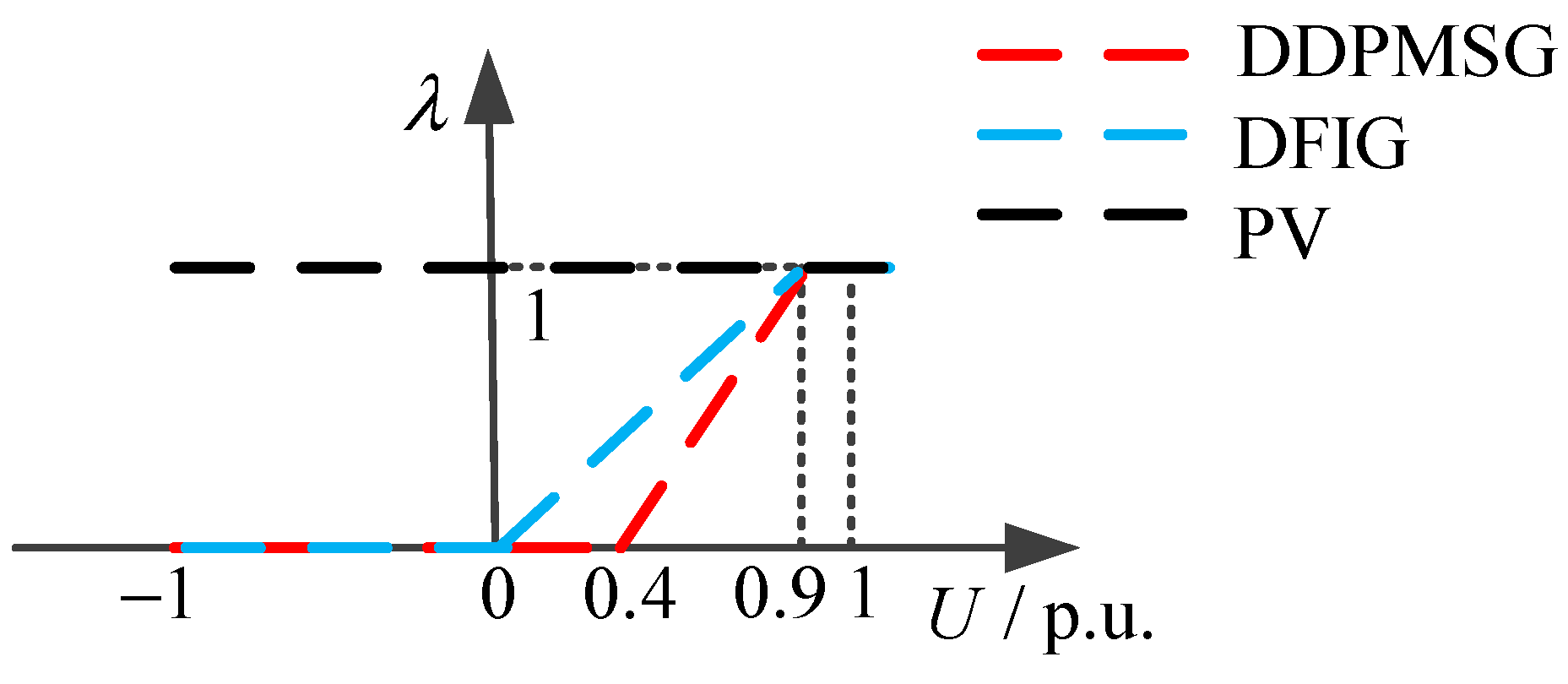
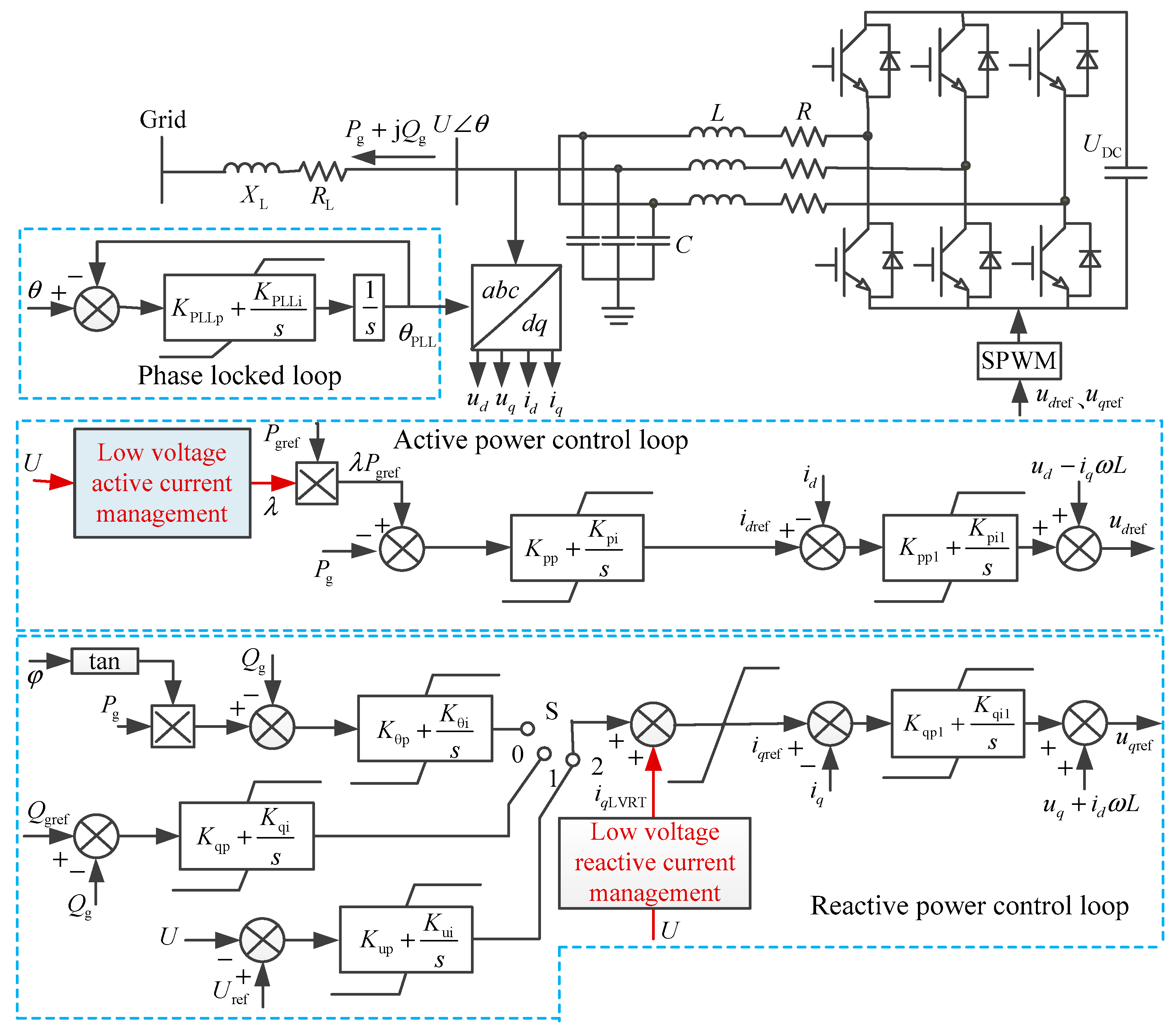
2.1. LVRT Control Strategy

The LVRT control includes two blocks labeled as low voltage active current management (LVACM) and low voltage reactive current management (LVRCM). They are used to mitigate the system stress during the fault, by limiting the current command with both an upper limit and a ramp rate limit. Generally, the reactive power priority control manner is used.

(1) LVRCM: The LVRCM function is designed to increase the reactive current under low voltage (smaller than $0.9U_{\mathrm{n}}$) scenarios. The renewable DG’s reactive current $i_{\mathrm{q}}$ is the sum of reactive current from normal control $i_{\mathrm{q}\_\mathrm{normal}}$ and the one from LVRCM module $i_{\mathrm{qLVRT}}$, namely:

$$i_{\mathrm{q}}=\min \left\{i_{\mathrm{q}\_\mathrm{normal}}+i_{\mathrm{qLVRT}},I_{\max }\right\}$$

(1)

In this paper, $I_{\max }$ is 1.1 p.u. for DDPMSG WT and DFIG WT, and 1.5 p.u. for the PV generation.

For DDPMSG WT, the reactive current of the LVRCM module $i_{q\mathrm{LVRT}}$ is,

$$i_{q\mathrm{LVRT}}=k_q\left(U_{\mathrm{n}}-U\right)=k_q\Delta U,0\le U\le 0.9U_{\mathrm{n}}$$

(2)

For the PV generation, the reactive current of the LVRCM module $i_{q\mathrm{LVRT}}$ is,

$$i_{q\mathrm{LVRT}}=\{\begin{array}{l}0,\hspace{1em}\left(U_{\mathrm{n}}-U\right)<0.2U_{\mathrm{n}}\\ k_q\left(U_{\mathrm{n}}-U\right)-0.25,\hspace{1em}\left(U_{\mathrm{n}}-U\right)\ge 0.2U_{\mathrm{n}}\end{array}$$

(3)

In (2) and (3), $k_q$ is the reactive support coefficient with the value of 0.8 for DDPMSG WT, and 2.5 for the PV generation.

(2) LVACM: The LVACM function adjusts the active power reference value, based on the terminal voltage of the renewable DG during the LVRT by $P_{\mathrm{LVRT}}=\lambda P_{\mathrm{ref}}$, and the coefficient is $\lambda$, Figure 1 depicts the LVACM control strategy.

Under the mode of the reactive power priority control, the active current during the LVRT can be expressed as follows,

$$i_d=\min \left\{\frac{P_{\mathrm{LVRT}}}{U},\sqrt{I_{\max }^2-i_q^2}\right\}$$

(4)

2.2. Dynamic Responses of the DGs

In order to analyze the dynamic characteristics of the different types of renewable DGs, simulations under a $20\%U_{\mathrm{n}}$ voltage dip are established. Figure 2 illustrates the transient responses of three types of DGs.

As shown in Figure 2, we have the following observations:

(1) All renewable DGs are at the LVRT state during the fault since the $20\%U_{\mathrm{n}}$ voltage dip exceeds the threshold voltage of the LVRT.

(2) During the voltage dip fault, the active power response trends of all renewable DGs are similar, and the difference is the active power value. Specifically, according to Figure 1, we have the following observations:

(a) The value $\lambda$ of DFIG WT is 0.88, indicating that its $P_{\mathrm{LVRT}}$ is 0.88 p.u.

(b) The $\lambda$ of DDPMSG WT is 0.8, therefore its active power $P_{\mathrm{LVRT}}$ is 0.8 p.u.

(c) The $P_{\mathrm{LVRT}}$ of the PV generation is around 0.96 p.u., since its coefficient $\lambda$ is 1.

(3) During the fault, the reactive power response trends of all renewable DGs are also similar to each other, and the difference is the reactive power value. Specifically, the reactive power of DFIG WT is 0, since it has no LVACM control, while the reactive power of DDPMSG WT and the PV generation will increase, according to (2) and (3).

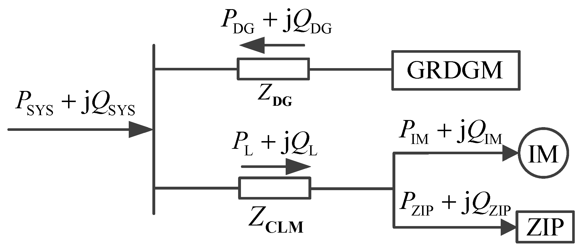
3. A General Model of the Multiple Renewable DGs

In this section, we present a general model for multiple renewable DGs. In particular, we first give a reduced order model for renewable DGs in Section 3.1 and then describe a general model of multiple renewable DGs in Section 3.2.

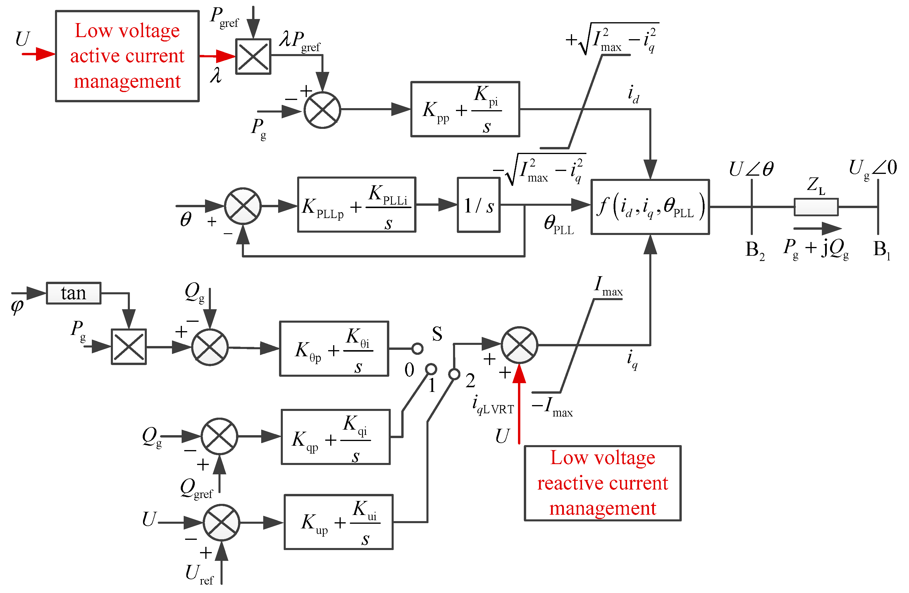
3.1. A Reduced Order Model for Renewable DGs

To analyze the dynamics of the ADN, an aggregate model with a low order and fewer computational time features is developed to investigate the dynamics of the different types of renewable DGs.

Since the dynamic responses are similar for different types of renewable DGs, it is reasonable to construct a general model. At the same time, the dynamics of renewable DGs are dominated by the converters and their control strategies, a simplification model can be attained, based on the order reduction technique, by which the components related to the non-dominate modes are neglected. The simplifications are as follows:

(1) The mechanical part of the wind turbine generators including the wind turbine, MPPT control, pitch angle control, and drive train are neglected.

(2) The generator and the grid-side converter are ignored as in Ref. [31].

With the simplification method above, the reduced order model of the renewable DGs is shown in Figure 3. It includes six components: the DC capacitor, the simplified phase-locked loop (PLL) model [32], the converter, the RLC filter element, the active current control with the LVACM, and the reactive current control with the LVRCM.

3.2. A General Model of the Multiple Renewable DGs

The dual-loop controller, which comprises an inner current loop and an outer power loop, is often used in the renewable DG’s control. Zhao et al. [33] showed that the time scale of the inner current controller is about 10 ms, while the outer power control and phase-locked control is about 100 ms. When the ADNs are modelled for the power system electro-mechanical transient analysis, the fast dynamics of the inner current control can be neglected by setting $i_d=i_{d\mathrm{ref}}$ and $i_q=i_{q\mathrm{ref}}$. The limit of each block in the active/reactive control loop is aggregated as one value.

To further simplify the renewable DG model in Figure 3, a current source model is used, in which, the converter and the filter are neglected, and the PLL is used to lock the phase. Based on these simplifications, the model illustrated in Figure 3 can be adjusted to the model, as shown in Figure 4, which is named as the general renewable DG model (GRDGM) in this paper.

In Figure 4, the function $f\left(i_d,i_q,{\theta }_{\mathrm{PLL}}\right)$ is expressed as:

$$f\left(i_d,i_q,{\theta }_{\mathrm{PLL}}\right)=(i_d+\mathrm{j}{i}_q)e^{\mathrm{j}{\theta }_{\mathrm{PLL}}}$$

(5)

The output power of the renewable DG is:

$$\{\begin{array}{l}{P}_g=i_{d}U\cos (\theta -{\theta }_{\mathrm{PLL}})+i_{q}U\sin (\theta -{\theta }_{\mathrm{PLL}})\\ Q_g=i_{d}U\sin (\theta -{\theta }_{\mathrm{PLL}})-i_{q}U\cos (\theta -{\theta }_{\mathrm{PLL}})\end{array}$$

(6)

In a steady state, $\theta ={\theta }_{\mathrm{PLL}}$.

4. Model Aggregation for Multiple DGs

Generally, the distribution network contains many types of renewable DGs, located at different sites, and their operation statuses are often different. Since the model of Figure 4 is generic for different types of renewable DGs, their equivalent model will have the same structure. The parameters of the linear modules in the equivalent model can be calculated by the system identification method. However, the nonlinear module, such as the LVACM and LVRCM, and the limit needs to be aggregated, based on the operation status of each renewable DG, which are shown in the following subsections.

4.1. Aggregation of the LVACM and LVRCM

According to Section 2, the active power reference value of the equivalent LVACM under the LVRT can be expressed as:

$$P_{\mathrm{eq}.\mathrm{ref}}={\displaystyle \sum _{j=1}^n\lambda \left(j\right)P_{g\mathrm{ref}}\left(j\right)=}{\lambda }_{\mathrm{eq}}{\displaystyle \sum _{j=1}^n{P}_{g\mathrm{ref}}\left(j\right)}$$

(7)

where $n$ is the number of renewable DGs in the ADN, $P_{\mathrm{eq}.\mathrm{ref}}$ and ${\lambda }_{\mathrm{eq}}$ are the reference values of active power and the power coefficient of the equivalent model, respectively. With the values of $P_{\mathrm{eq}.\mathrm{ref}}$ and ${\displaystyle \sum _{j=1}^n{P}_{\mathrm{gref}}(j)}$, ${\lambda }_{\mathrm{eq}}$ of the equivalent model can be obtained.

Based on (2) and (3), the reactive current of the equivalent LVRCM can be expressed as:

$$i_{q\mathrm{LVRT}.\mathrm{eq}}={\displaystyle \sum _{j=1}^n{k}_q\left(j\right)\Delta U\left(j\right)}=k_{q.\mathrm{eq}}\Delta U_{\mathrm{eq}}$$

(8)

where parameter $k_{q.\mathrm{eq}}$ can be calculated by $k_q$ and $\Delta U$ of each renewable DG, and also by the voltage variation $\Delta U_{\mathrm{eq}}$ of the equivalent bus under a certain disturbance.

4.2. Determination of the Current Limit for the Equivalent Model

Assuming that $I_{\max }$ is the current limit value of a single renewable DG and $I_{\max .\mathrm{eq}}$ is the current limit of the equivalent model, we have

(1) When the current of all renewable DGs is less than the limit value, $I_{\max .\mathrm{eq}}$ can be calculated through:

$$\{\begin{array}{l}{i}_{q.\mathrm{eq}}={\displaystyle \sum _{j=1}^n{i}_q\left(j\right)}\\ i_{d.\mathrm{eq}}={\displaystyle \sum _{j=1}^n{i}_d\left(j\right)}={\displaystyle \sum _{j=1}^n\sqrt{I_{\max }{\left(j\right)}^2-i_q^2\left(j\right)}}=\sqrt{I_{\max .\mathrm{eq}}^2-i_{q.\mathrm{eq}}^2}\end{array}$$

(9)

(2) When the currents of $n_1$ renewable DGs exceed their limits, and the currents of $(n-n_1)$ renewable DGs are less than the limits, $I_{\max .\mathrm{eq}}$ can be calculated through:

$$\{\begin{array}{l}{i}_{q.\mathrm{eq}}={\displaystyle \sum _{j=1}^{n_1}{I}_{\max }\left(j\right)}+{\displaystyle \sum _{j=n_1+1}^n{i}_q\left(j\right)}\\ i_{d.\mathrm{eq}}={\displaystyle \sum _{j=n_1+1}^n{i}_d\left(j\right)}={\displaystyle \sum _{j=n_1+1}^n\sqrt{I_{\max }{\left(j\right)}^2-i_q^2\left(j\right)}}=\sqrt{I_{\max .\mathrm{eq}}^2-i_{q.\mathrm{eq}}^2}\end{array}$$

(10)

(3) When all renewable DGs exceed their limits, we have $i_{d.\mathrm{eq}}=0$, and $I_{\max .\mathrm{eq}}$ reaches the maximum value, i.e.,

$$I_{\max .\mathrm{eq}}={\displaystyle \sum _{j=1}^n{I}_{\max }\left(j\right)}$$

(11)

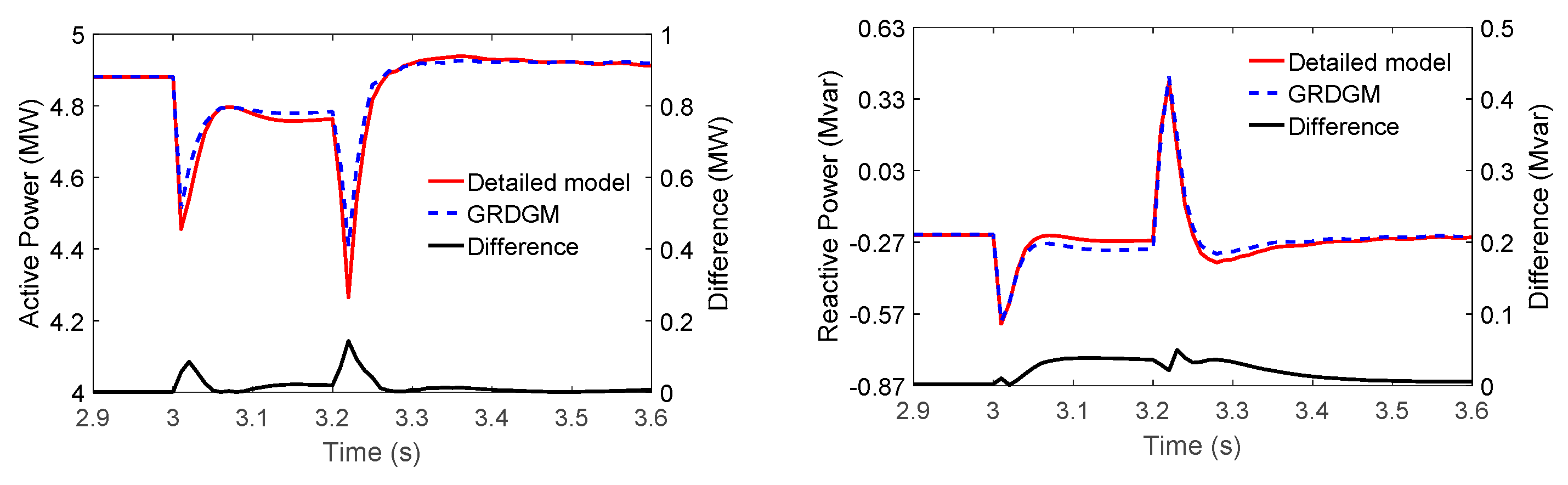
5. Effectiveness of the GRDGM for Describing Multiple Types of Renewable DGs

To validate the effectiveness of the GRDGM representing the aggregate dynamic behavior of the multiple renewable DGs in the distribution network, the case with three types of DGs, as shown in Figure 5, is applied. The overall responses of the three renewable DGs, based on the detailed model are compared with the ones from the GRDGM.

The system as shown in Figure 5 consists of three types of renewable DGs connected to the infinite source through transmission lines ($Z_{\mathrm{L}1}$, $Z_{\mathrm{L}2}$) and two transformers ($Z_{\mathrm{T}1}$, $Z_{\mathrm{T}2}$). The rated power of DFIG WT, DDPMSG WT and PV are 2 MW, 2 MW and 1 MW, respectively, and their grid-connected impedance are $Z_1=0.5765+\mathrm{j}1.6485\Omega$, $Z_2=4.6120+\mathrm{j}13.1880\Omega$ and $Z_3=6.3415+\mathrm{j}18.1335\Omega$, respectively. Assuming that all renewable DGs are with constant reactive power control mode, the LVACM and LVRCM are the same as in Section 2.1. The remaining parameters are the same with the recommended values on simulation platform of PSCAD/EMTDC [23,24,25].

The parameters {$K_{\mathrm{pp}}$, $K_{\mathrm{pi}}$, $K_{\mathrm{qp}}$, $K_{\mathrm{qi}}$, $K_{\mathrm{PLLp}}$, $K_{\mathrm{PLLi}}$} in GRDGM, and the impedance $Z_{\mathrm{eq}}$ between equivalent renewable DG and bus B₂ are required to be estimated. They can be estimated by the curve fitting method, which can be achieved through:

$$\min \mathrm{error}=\frac{1}{K}{\displaystyle \sum _{i=1}^{i=K}\left[{(\frac{P_{\mathrm{sim}}(i)-P_{\mathrm{real}}(i)}{P_{\mathrm{real}}(i)})}^2+{(\frac{Q_{\mathrm{sim}}(i)-Q_{\mathrm{real}}(i)}{Q_{\mathrm{real}}(i)})}^2\right]}$$

(12)

where P_sim and Q_sim are the active and reactive power responses, based on the general model, respectively; P_real and Q_real are the active and reactive power, based on the detailed model, respectively; K is the total number of points in the time window of the disturbed trajectory. The sampling step is 10⁻⁵ s, and the simulation platform is PSCAD.

According to the grid-connected impedance of all renewable DGs in Figure 5, the threshold value of the LVRT and the current limit of each renewable DG, we can attain that:

(1) all renewable DGs will not enter into the LVRT state when the voltage of B₂ is larger than 89.8%U_n;

(2) all renewable DGs will enter into the LVRT when the voltage of B₂ is lower than 78.1%U_n;

(3) all renewable DGs will exceed the current limit when the voltage of B₂ is lower than 59.2%U_n.

5.1. Parameter Estimation Results

To estimate the parameters in the GRDGM, a 9.5%U_n voltage dip disturbance is conducted at B₁ through the adjustment of the grounding resistance, the fault lasts for 0.2 s and the system returns to its original state after clearing the fault. Under this fault, all renewable DGs will not enter the LVRT state, and the converter’s current is within the limit. Therefore, the values of the equivalent LVACM and LVRCM will be λ_eq = 1, k_q.eq = 0, respectively, based on (7) and (8).

The total real and reactive power responses of three renewable DGs with a detailed model at B_2, are used as the training data, in order to obtain model parameters by means of curve fitting, based on (12). The curve fitting method is a particle swarm optimization algorithm. The initial population number of the particles and the learning factor are assumed to be 20 and 2, respectively, and the maximum number of iterations is 200. The identification results are shown in

Table 1. Estimated results of parameters in GRDGM.

Parameter	Estimation	Parameter	Estimation
$R_{\mathrm{eq}}$(Ω)	3.5117	$X_{\mathrm{eq}}$(Ω)	5.4950
$K_{\mathrm{pp}}$	8.5231	$K_{\mathrm{pi}}$	0.07509
$K_{\mathrm{qp}}$	1.3200	$K_{\mathrm{qi}}$	0.1177
$K_{\mathrm{PLLp}}$	68.9987	$K_{\mathrm{PLLi}}$	2500.3433

.

The responses of the GRDGM and the detailed model are demonstrated in Figure 6, and the fitting error of (12) is 0.0031. It can be seen that the GRDGM can well capture the whole dynamics of the multi-type renewable DGs.

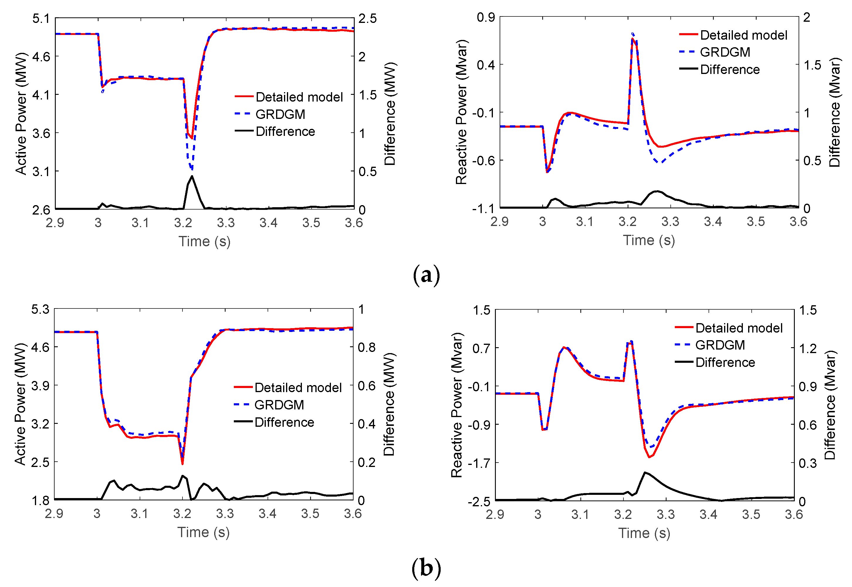
5.2. Adaptability of the GRDGM

To further verify the adaptability of the GRDGM, we conduct two other disturbance scenarios, as follows.

Scenario 1: the disturbance with an 18.5%U_n voltage dip at B₂.

Scenario 2: the disturbance with a 39%U_n voltage dip at B₂.

In both, the duration of the voltage drops is 0.2 s. Meanwhile, the parameters obtained from the 9.5%U_n voltage dip disturbance are used to fit the responses of these two disturbances.

According to the grid-connected impedances of three DGs, it can be obtained that the DFIG WT and the DDPMSG WT will enter into LVRT under both disturbance scenarios. Parameters of the equivalent LVACM and LVRCM are calculate based on (7) and (8), and resulted as ${\lambda }_{\mathrm{eq}}$ = 0.9087, $k_{q.\mathrm{eq}}$ = 0.3167 and ${\lambda }_{\mathrm{eq}}$ = 0.6474, $k_{q.\mathrm{eq}}$ = 0.6659 for each scenario, respectively. In addition, the currents of DFIG WT and the DDPMSG WT will exceed the limits, and the limiting value of the equivalent model is $I_{\max .\mathrm{eq}}=1.18 \mathrm{p}.\mathrm{u}.$ based on (10).

The overall responses of the three renewable DGs under the obtained parameters from the $9.5\%U_{\mathrm{n}}$ voltage dip disturbance are shown in Figure 7. In Figure 7a, the fitting error of (12) is 0.0181; while in Figure 7b, the error is 0.0389.

It can be seen from Figure 7 that the GRDGM has a high accuracy in fitting the overall dynamics of the multiple types of renewable DGs. Moreover, the estimated parameters under one disturbance have a good adaptability to other disturbances.

6. General Model of the ADN

In this section, we investigate the general model of the ADN. In particular, the initial stages of the model development for the ADN focuses on constructing the general model for the multiple renewable DGs. Then, the equivalent modeling for the ADN with various types of renewable DGs will be investigated.

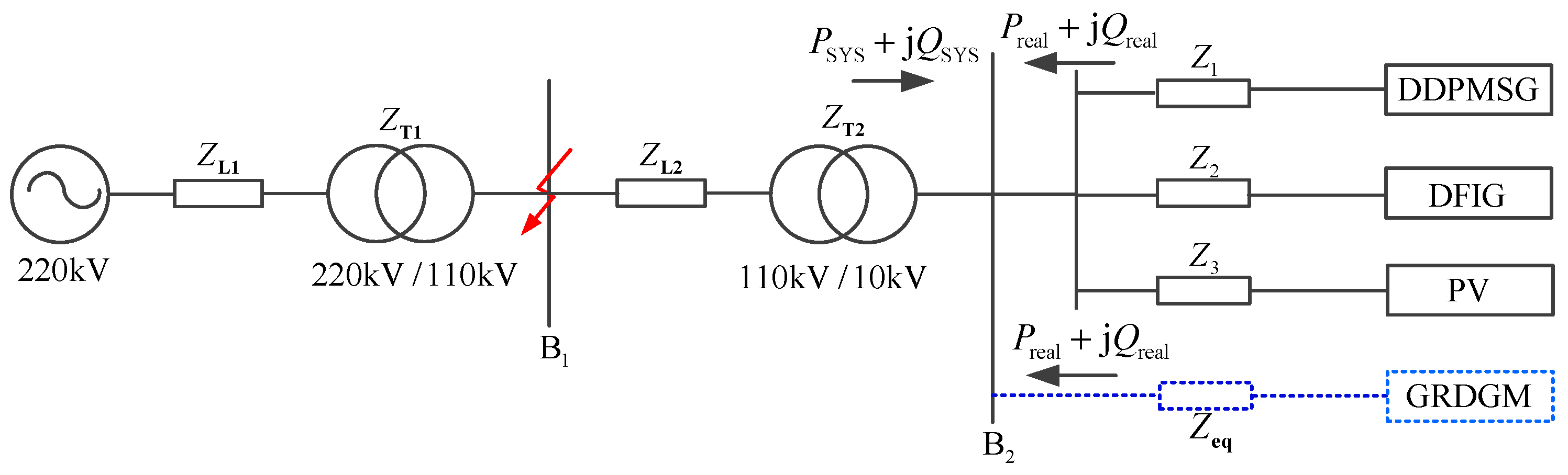
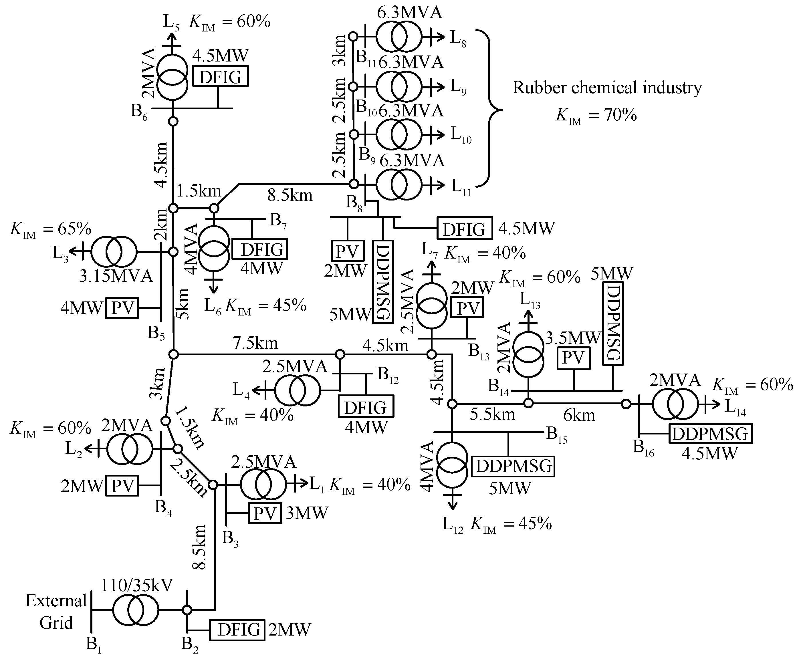
6.1. General ADN Model

The general ADN model (GADNM) can be represented by the parallel connection of the traditional CLM and the GRDGM, as shown in Figure 8.

In Figure 8, ZIP is the static load, and IM is induction motor load. When the power loss is neglected, Figure 8 satisfies,

$$\{\begin{array}{l}{P}_{\mathrm{L}}=P_{\mathrm{IM}}+P_{\mathrm{ZIP}}=P_{\mathrm{DG}}+P_{\mathrm{SYS}}\\ Q_{\mathrm{L}}=Q_{\mathrm{IM}}+Q_{\mathrm{ZIP}}=Q_{\mathrm{DG}}+Q_{\mathrm{SYS}}\end{array}$$

(13)

The proportion of renewable DG’s power $K_{\mathrm{DG}}$ and the proportion of dynamic load $K_{\mathrm{IM}}$ can be defined as follows,

$$\{\begin{array}{l}{K}_{\mathrm{DG}}=P_{\mathrm{DG}}/P_{\mathrm{L}}\\ K_{\mathrm{IM}}=P_{\mathrm{IM}}/P_{\mathrm{L}}\end{array}$$

(14)

The system delivers power to the load when $K_{\mathrm{DG}}<1$, while the ADN delivers power to the system when $K_{\mathrm{DG}}>1$.

6.2. Case Study

A real 35 kV active distribution network of an industrial park in China, shown in Figure 9 is used to evaluate the performance of the GADNM. The system is built on the PSCAD/EMTDC platform, the resistance, and reactance of the cable line per kilometer are 0.116 Ω/km and 0.10676 Ω/km, respectively. Since the park is dominated by civil light industry load, e.g., rubber, plastics, and related manufacturers, most induction motors are small ones. In Figure 9, the parameters of the induction motors are set with the same value, which are as follows, stator resistance and reactance are $R_{\mathrm{s}}=0.078 \mathrm{p}.\mathrm{u}.$, $X_{\mathrm{s}}=0.065 \mathrm{p}.\mathrm{u}.$, respectively; rotor’s resistance and reactance are $R_{\mathrm{r}}=0.044 \mathrm{p}.\mathrm{u}.$ and $X_{\mathrm{r}}=0.069 \mathrm{p}.\mathrm{u}.$, respectively; and its inertial time constant and excitation reactance are $H=1 \mathrm{s}$ and $X_{\mathrm{m}}=2.67 \mathrm{p}.\mathrm{u}.$, respectively. The static load adopts the constant impedance model, and the ratio of resistance/reactance is 5.

In the steady state, $K_{\mathrm{DG}}=1$, and the output power of DFIG WT, DDPMSG WT, and PV accounts for 34.48%, 35.39%, and 30.12% of the total DG power, respectively.

To verify the proposed GADNM, two disturbances with $20\%U_{\mathrm{n}}$ and $70\%U_{\mathrm{n}}$ voltage dip at ${\mathrm{B}}_2$ are established. In both disturbances, the duration time of voltage drop is 0.2 s. The responses of $20\%U_n$ voltage dip disturbance is used to estimate the model parameters by means of curve fitting, then the estimated parameters are used to fit the responses of $70\%U_n$ voltage dip disturbance to validate the model adaptability.

As shown in Figure 9, 15 parameters {$R_{\mathrm{DG}}$, $X_{\mathrm{DG}}$, $R_{\mathrm{CLM}}$, $X_{\mathrm{CLM}}$, $K_{\mathrm{pp}}$, $K_{\mathrm{pi}}$, $K_{\mathrm{qp}}$, $K_{\mathrm{qi}}$, $K_{\mathrm{PPLp}}$, $K_{\mathrm{PPLi}}$, $X_{\mathrm{s}}$, $H$, $s_0$, $K_{\mathrm{DG}}$, $K_{\mathrm{IM}}$} need to be estimated. Among them, $s_0$ is the initial slip of induction motor. The active and reactive power at bus B₂ is used for curve fitting, and the particle swarm optimization algorithm is used for parameter estimation.

Under the disturbance of $20\%U_{\mathrm{n}}$ voltage dip, we have ${\lambda }_{\mathrm{eq}}$ = 0.9132 and $k_{q.\mathrm{eq}}$ = 0.2713 based on (7) and (8). Under the disturbance of $70\%U_n$ voltage dip, we have ${\lambda }_{\mathrm{eq}}$ = 0.4261 and $k_{q.\mathrm{eq}}$ = 0.9014. For both disturbances, $I_{\max .\mathrm{eq}}$ is 1.2179 p.u. based on (11).

Figure 10 shows the responses of active power and reactive power at bus ${\mathrm{B}}_2$ from the detailed model as shown in Figure 9 and the GADNM model as shown in Figure 8. As shown in Figure 10a, the error of (12) is 0.0530, while in Figure 10b, the error of (12) is 0.0864. The estimation results of 15 parameters are shown in

Table 2. Estimated results of the parameters in the GADNM.

Parameter	Estimation	Parameter	Estimation
$R_{\mathrm{DG}}$(Ω)	3.4221	$X_{\mathrm{DG}}$(Ω)	4.3953
$K_{\mathrm{pp}}$	2.8821	$K_{\mathrm{pi}}$	0.1291
$K_{\mathrm{qp}}$	1.1114	$K_{\mathrm{qi}}$	0.3437
$K_{\mathrm{PPLp}}$	114.1579	$K_{\mathrm{PPLi}}$	2791.2335
$R_{\mathrm{CLM}}$(Ω)	5.7222	$X_{\mathrm{CLM}}$(Ω)	6.5241
$X_{\mathrm{s}}$(p.u.)	0.0599	$H$(s)	1.0812
$s_0$(%)	1.6774	\	\
$K_{\mathrm{IM}}$(%)	64.1446	$K_{\mathrm{DG}}$(%)	102.3873

.

6.3. Adaptability Analysis

Three scenarios with $K_{\mathrm{DG}}=20\%$, $K_{\mathrm{DG}}=50\%$ and $K_{\mathrm{DG}}=100\%$ under different voltage dip disturbances are conducted to investigate the model adaptability. The estimated parameters in Section 6.2 are used to fit the responses. Figure 11, Figure 12 and Figure 13 show the results.

We next present the detailed results, according the three scenarios, as follows.

(1) $K_{\mathrm{DG}}=20\%$

(2) $K_{\mathrm{DG}}=50\%$

(3) $K_{\mathrm{DG}}=200\%$

Under the three renewable DG penetration scenarios, the fitting errors are 0.0372, 0.0592, and 0.0794 under the $20\%U_{\mathrm{n}}$ voltage dip disturbance, respectively, and the errors are 0.0913, 0.0944, and 0.1004, respectively, under the $70\%U_{\mathrm{n}}$ voltage dip disturbance.

Based on the above analysis, it can be concluded that the proposed GADNM can achieve a high accuracy when it simulates the overall dynamic process of the ADN under various scenarios and voltage dip disturbances.

7. Conclusions

Due to the complexity of the detailed models of the different renewable DGs, including the DFIG WT, DDPMSG WT, and PV generations, the diversities of their location and operation status, this paper proposes a general GRDGM model to study the different types of renewable DGs, based on the similarity of their model structure and dynamic characteristics. The GRDGM is validated by comparing its responses with the detailed models of various renewable DGs, and both the feasibility and adaptability of the GRDGM are also verified.

Furthermore, the proposed GRDGM is connected in parallel with the traditional CLM, as the dynamic model structure of the ADN. The model is also validated, based on an actual ADN with multiple renewable DGs, and the results show that the proposed GADNM has a good adaptability under different DG penetration levels and different voltage dip disturbances.

References

1. Kosterev, D.N.; Taylor, C.W.; Mittelstadt, W.A. Model validation for the August 10, 1996 WSCC system outage. IEEE Trans. Power Syst. 1999, 14, 967–979. [Google Scholar] [CrossRef] [PubMed] [Green Version]
2. Arif, A.; Wang, Z.; Wang, J.; Mather, B.; Bashualdo, H.; Zhao, D. Load modeling—A review. IEEE Trans. Smart Grid 2018, 9, 5986–5999. [Google Scholar] [CrossRef]
3. Milanovic, J.V.; Yamashita, K.; Martínez Villanueva, S.; Djokic, S.Ž.; Korunović, L.M. International industry practice on power system load modeling. IEEE Trans. Power Syst. 2013, 28, 3038–3046. [Google Scholar] [CrossRef]
4. Kosterev, D.; Meklin, A.; Undrill, J.; Lesieutre, B.; Price, W.; Chassin, D.; Bravo, R.; Yang, S. Load modeling in power system studies: WECC progress update. In Proceedings of the IEEE PES General Meeting, Pittsburgh, PA, USA, 20–24 July 2008; pp. 1–8. [Google Scholar]
5. Paidi, E.S.N.R.; Nechifor, A.; Albu, M.M.; Yu, J.; Terzija, V. Development and validation of a new oscillatory component load model for real-time estimation of dynamic load model parameters. IEEE Trans. Power Deliv. 2020, 35, 618–629. [Google Scholar] [CrossRef]
6. Chen, D.; Mohler, R.R. Neural-network-based load modeling and its use in voltage stability analysis. IEEE Trans. Control Syst. Technol. 2003, 11, 460–470. [Google Scholar] [CrossRef]
7. Ma, Z.; Wang, Z.; Wang, Y.; Diao, R.; Shi, D. Mathematical representation of WECC composite load model. J. Mod. Power Syst. Clean Energy 2020, 8, 1015–1023. [Google Scholar] [CrossRef]
8. Mat Zali, S.; Milanović, J.V. Generic model of active distribution network for large power system stability studies. IEEE Trans. Power Syst. 2013, 28, 3126–3133. [Google Scholar] [CrossRef]
9. Zheng, C.; Wang, S.; Liu, Y.; Liu, C. A novel RNN based load modelling method with measurement data in active distribution system. Electr. Power Syst. Res. 2019, 166, 112–124. [Google Scholar] [CrossRef]
10. Zaker, B.; Gharehpetian, G.B.; Karrari, M. A novel measurement-based dynamic equivalent model of grid-connected microgrids. IEEE Trans. Ind. Inf. 2019, 15, 2032–2043. [Google Scholar] [CrossRef]
11. Wang, P.; Zhang, Z.; Huang, Q.; Tang, X.; Lee, W.-J. Robustness-improved method for measurement-based equivalent modeling of active distribution network. IEEE Trans. Ind. Appl. 2021, 57, 2146–2155. [Google Scholar] [CrossRef]
12. Milanović, J.V.; Mat Zali, S. Validation of equivalent dynamic model of active distribution network cell. IEEE Trans. Power Syst. 2013, 28, 2101–2110. [Google Scholar] [CrossRef]
13. Conte, F.; D’Agostino, F.; Silvestro, F. Operational constrained nonlinear modeling and identification of active distribution networks. Electr. Power Syst. Res. 2019, 168, 92–104. [Google Scholar] [CrossRef]
14. Matevosyan, J.; Martínez Villanueva, S.; Djokic, S.Z.; Acosta, J.L.; Mat Zali, S.; Resende, F.O.; Milanovic, J.V. Aggregated models of wind-based generation and active distribution network cells for power system studies—Literature overview. In Proceedings of the 2011 IEEE Trondheim PowerTech, Trondheim, Norway, 19–23 June 2011; pp. 1–8. [Google Scholar]
15. Ramasubramanian, D.; Yu, Z.; Ayyanar, R.; Vittal, V.; Undrill, J. Converter model for representing converter interfaced generation in large scale grid simulations. IEEE Trans. Power Syst. 2017, 32, 765–773. [Google Scholar] [CrossRef]
16. Pourbeik, P. Proposal for the DER_A model. In Presentation WECC Meet. 2016. Available online: https://www.wecc.biz/Reliability/DER_A_Final.pdf (accessed on 20 July 2022).
17. Takenobu, Y.; Akagi, S.; Ishii, H.; Hayashi, Y.; York, B.; Ramasubramanian, D.; Mitra, P.; Gaikwad, A.; York, B. Evaluation of dynamic voltage responses of distributed energy resources in distribution systems. In Proceedings of the 2018 IEEE Power & Energy Society General Meeting (PESGM), Portland, OR, USA, 5–10 August 2018; pp. 1–5. [Google Scholar]
18. Li, Y.; Hu, S.; Zhang, X.; Tian, P. Dynamic equivalent of inverter-based distributed generations for large voltage disturbances. Energy Rep. 2022, 8, 14488–14497. [Google Scholar] [CrossRef]
19. Ishchenko, A.; Jokic, A.; Myrzik, J.M.A.; Kling, W.L. Dynamic reduction of distribution networks with dispersed generation. In Proceedings of the 2005 International Conference on Future Power Systems, Amsterdam, The Netherlands, 18 November 2005; pp. 1–7. [Google Scholar]
20. Ishchenko, A.; Myrzik, J.M.A.; Kling, W.L. Dynamic equivalencing of distribution networks with dispersed generation using Hankel norm approximation. IET Gen. Transm. Distrib. 2007, 1, 818–825. [Google Scholar] [CrossRef]
21. Collin, A.J.; Tsagarakis, G.; Kiprakis, A.E.; McLaughlin, S. Development of Low-Voltage Load Models for the Residential Load Sector. IEEE Trans. Power Syst. 2014, 29, 2180–2188. [Google Scholar] [CrossRef]
22. Yang, D.; Wang, B.; Cai, G.; Chen, Z.; Ma, J.; Sun, Z.; Wang, L. Data-driven estimation of inertia for multiarea interconnected power systems using dynamic mode decomposition. IEEE Trans. Ind. Inf. 2021, 17, 2686–2695. [Google Scholar] [CrossRef]
23. Ku, B.-Y.; Thomas, R.J.; Chiou, C.-Y.; Lin, C.-J. Power system dynamic load modeling using artificial neural networks. IEEE Trans. Power Syst. 1994, 9, 1868–1874. [Google Scholar] [CrossRef]
24. Keyhani, A.; Lu, W.; Heydt, G.T. Composite neural network load models for power system stability analysis. In Proceedings of the IEEE PES Power Systems Conference and Exposition, New York, NY, USA, 10–13 October 2004; pp. 1159–1163. [Google Scholar]
25. Chávarro-Barrera, L.; Pérez-Londoño, S.; Mora-Flórez, J. An adaptive approach for dynamic load modeling in microgrids. IEEE Trans. Smart Grid 2021, 12, 2834–2843. [Google Scholar] [CrossRef]
26. Li, W.; Chao, P.; Liang, X.; Xu, D.; Jin, W. An improved single-machine equivalent method of wind power plants by calibrating power recovery behaviors. IEEE Trans. Power Syst. 2018, 33, 4371–4381. [Google Scholar] [CrossRef]
27. Chao, P.; Li, W.; Peng, S.; Liang, X.; Zhang, L.; Shuai, Y. Fault ride-through behaviors correction-based single-unit equivalent method for large photovoltaic power plants. IEEE Trans. Sustain. Energy 2021, 12, 715–726. [Google Scholar] [CrossRef]
28. Manitoba Hydro International Ltd., Winnipeg, Manitoba, Canada, 2019. Simple Solar Farm 2019, Revision 2. Available online: https://www.pscad.com/knowledge-base/article/521 (accessed on 20 July 2022).
29. Manitoba Hydro International Ltd., Winnipeg, Manitoba, Canada, 2018a. Type 3 Wind Turbine Model, Revision 3. Available online: https://www.pscad.com/knowledge-base/article/496 (accessed on 20 July 2022).
30. Manitoba Hydro International Ltd., Winnipeg, Manitoba, Canada, 2018b. Type 4 Wind Turbine Model, Revision 3. Available online: https://www.pscad.com/knowledge-base/article/227 (accessed on 20 July 2022).
31. Pourbeik, P.; Sanchez-Gasca, J.J.; Senthil, J.; Weber, J.D.; Zadehkhost, P.S.; Kazachkov, Y.; Tacke, S.; Wen, J.; Ellis, A. Generic dynamic models for modeling wind power plants and other renewable technologies in large-scale power system studies. IEEE Trans. Energy Convers. 2017, 32, 1108–1116. [Google Scholar] [CrossRef]
32. Golestan, S.; Guerrero, J.M. Conventional synchronous reference frame phase-locked loop is an adaptive complex filter. IEEE Trans. Ind. Electron. 2015, 62, 1679–1682. [Google Scholar] [CrossRef] [Green Version]
33. Zhao, M.; Yuan, X.; Hu, J.; Yan, Y. Voltage dynamics of current control time-scale in a VSC-connected weak grid. IEEE Trans. Power Syst. 2016, 31, 2925–2937. [Google Scholar] [CrossRef]
Figure 1. Low-voltage active power management.
Energies 15 08931 g001
Figure 2. Dynamic responses of three types of DGs.
Energies 15 08931 g002
Figure 3. A reduced order model structure for various types of renewable DGs.
Energies 15 08931 g003
Figure 4. The general renewable DG model.
Energies 15 08931 g004
Figure 5. Grid-connected diagram of the three DGs.
Energies 15 08931 g005
Figure 6. The renewable DGs’ responses under a 9.5%Un voltage dip.
Energies 15 08931 g006
Figure 7. Model adaptability analysis. (a) 18.5 % U n voltage dip disturbance at B2. (b) 39 % U n voltage dip disturbance at B2.
Energies 15 08931 g007
Figure 8. General ADN model.
Energies 15 08931 g008
Figure 9. Structure of a real 35 kV ADN.
Energies 15 08931 g009
Figure 10. Responses of two voltage dip disturbances with K DG = 100 % . (a) 20 % U n voltage dip. (b) 70 % U n voltage dip.
Energies 15 08931 g010
Figure 11. Responses of the two voltage dip disturbances with K DG = 20 % . (a) 20 % U n voltage dip. (b) 70 % U n voltage dip.
Energies 15 08931 g011
Figure 12. Responses of the two voltage dip disturbances with K DG = 50 % . (a) 20 % U n voltage dip. (b) 70 % U n voltage dip.
Energies 15 08931 g012
Figure 13. Responses of the two voltage dip disturbances with K DG = 200 % . (a) 20 % U n voltage dip. (b) 70 % U n voltage dip.
Energies 15 08931 g013