A Composite Variable Structure PI Controller for Sensorless Speed Control Systems of IPMSM

Abstract

In the speed control system of an Interior Permanent Magnet Synchronous Motor (IPMSM) without a speed sensor, PI controllers using only a fixed set of parameters cannot achieve accurate tracking of the estimated speed in a wide speed domain and also suffer from step response overshoot. This paper proposes a Compound Variable Structure PI (CVSPI) controller to improve the system control performance. It can choose whether to include an integral term according to the size of the system deviation to speed up the response. It also introduces a Model Reference Adaptive System (MRAS) speed observer in the controller to estimate the speed and adaptively adjust the size of the anti-integration saturation gain to improve the dynamic response following performance and immunity of the system. A feed-forward link is added for a given input differential to achieve an accurate answer to time-varying inputs. As the linear compensation matrix of the conventional MRAS is a unit matrix, the speed can only be accurately observed in a specific speed range. In this paper, a new linear compensation matrix is designed, and a new speed adaptive law is derived, allowing the improved MRAS to measure speed over a wide range accurately. Simulation results validate the excellent control performance of the CVSPI and the accuracy of the enhanced MRAS over a wide speed range.

1. Introduction

Interior Permanent Magnet Synchronous Motor (IPMSM) is widely used in industrial speed control systems for its high power/weight ratio, high torque/inertia ratio, high efficiency, and certain robustness [1,2,3]. Although a range of superior and complicated control techniques such as non-linear PI control [4], adaptive control, and sliding mode variable shape control has been utilized in the velocity loop [5], these non-linear control techniques have issues such as hard parameter adjustment or jitter. They need to be further improved [6]. Therefore, the dominant control method in industrial applications is still traditional PI control [7,8,9]. The conventional PI control is designed based on linear system theory [10], and a fixed set of PI parameters will cause a contradiction between the system’s steady-state performance and dynamic performance [11], making it difficult to take into account the steady-state performance and dynamic performance of the system at the same time [12]. Due to the physical constraints of the motor and inverter, limits must be placed on the system control inputs to protect the system [13]. When the controller output is limited by saturation due to an increase in the accumulation of the integral term (as can happen when there is a step response or sudden changes in load), a phenomenon known as Windup occurs [14,15,16]. This leads to a decline in the performance of the closed-loop system (e.g., a larger overshoot, a longer regulation time, and even the system losing stability). Therefore, the traditional PI controller can no longer meet the requirements of industrial automation for time-varying speed tracking and robustness in real time [17]. At the same time, the actual speed feedback in a closed loop system is mainly obtained indirectly by differentiating the mechanical angle of the rotor detected by the position sensor [18]. The installation of position sensors increases the motor’s size and cost, increases the rotor’s inertia [19,20], is prone to failure in complex environments, affects the dynamic and static performance of the system, and reduces the system’s robustness [21]. Therefore, the use of position sensors needs to be abandoned, and a speed sensor-less control strategy adopted to enhance the closed-loop system’s performance and the speed feedback’s accuracy [22].

In [23], a variable gain PI controller is proposed to automatically select the optimum gain for a given rate of change and thus achieve good speed tracking performance. However, as the gain of the PI controller changes in real time, it is impossible to avoid the fluctuation of the system speed for a given speed change. To improve the system’s performance against external load disturbances, [24] uses a non-linear disturbance observer to estimate the load torque and then adaptively adjust the fractional order PI parameters. Although this method is effective, the design process requires consideration of many non-ideal factors, and the algorithm is complex and not very practical. After analyzing the link between PI controller parameters and zero poles of the system, [25] proposes a PI controller parameter modification approach based on the pole arrangement that effectively dampens mechanical vibration when operating with flexible loads. However, the PI parameter tuning in this method only addresses the mechanical vibration problem of the system, and the tracking performance of the continuously changing input of the system has not been considered. The authors of [26] introduce an active disturbance rejection controller (ADRC) for speed regulation to compensate for disturbances inside and outside the IPMSM. Still, the parameter tuning of the ADRC is too tricky, and the tracking performance for different states of speed given is not universal. In [27], a fast super-distortion algorithm is proposed for the poor robustness of PI controllers in speed control systems and the problem of excessive jitter arrays in traditional sliding mode control, which has better immunity but lags in the tracking of time-varying signals [26,28].

This work offers a Compound Variable Structure PI (CVSPI) controller and an upgraded Model Reference Adaptive System (MRAS) speed to increase the control accuracy of the IPMSM speed sensorless speed control system in a wide range of speeds domain. The CVSPI can adjust the inclusion of the integration term according to the magnitude of the speed error to accelerate the start-up speed. Using the concept of inverse calculation compensation, the estimated rate is input into the anti-integration saturation gain in order to reduce step response exceedance. Additionally, the performance of the tacho loop tracking response is improved by the inclusion of a specified input differential feed-forward connection, which allows for a more precise reaction to input signals that change over time. To address the limitation of the stator current-based MRAS to provide reliable estimates of speed only at moderate and high frequencies, a linear compensation matrix incorporating inductive characteristics substitutes for the unit matrix.

This paper is organized as follows. Section 2 presents the design of the CVSPI and analyses its advantages and performance. Section 3 demonstrates that the linear compensation matrix with inductive parameters satisfies the conditions for Popov super stability and derives a new speed adaptive law. Section 4 carries out simulation experiments and analyses to validate the proposed method. Finally, Section 5 concludes the paper.

2. Composite Variable Structure PI Speed Controller

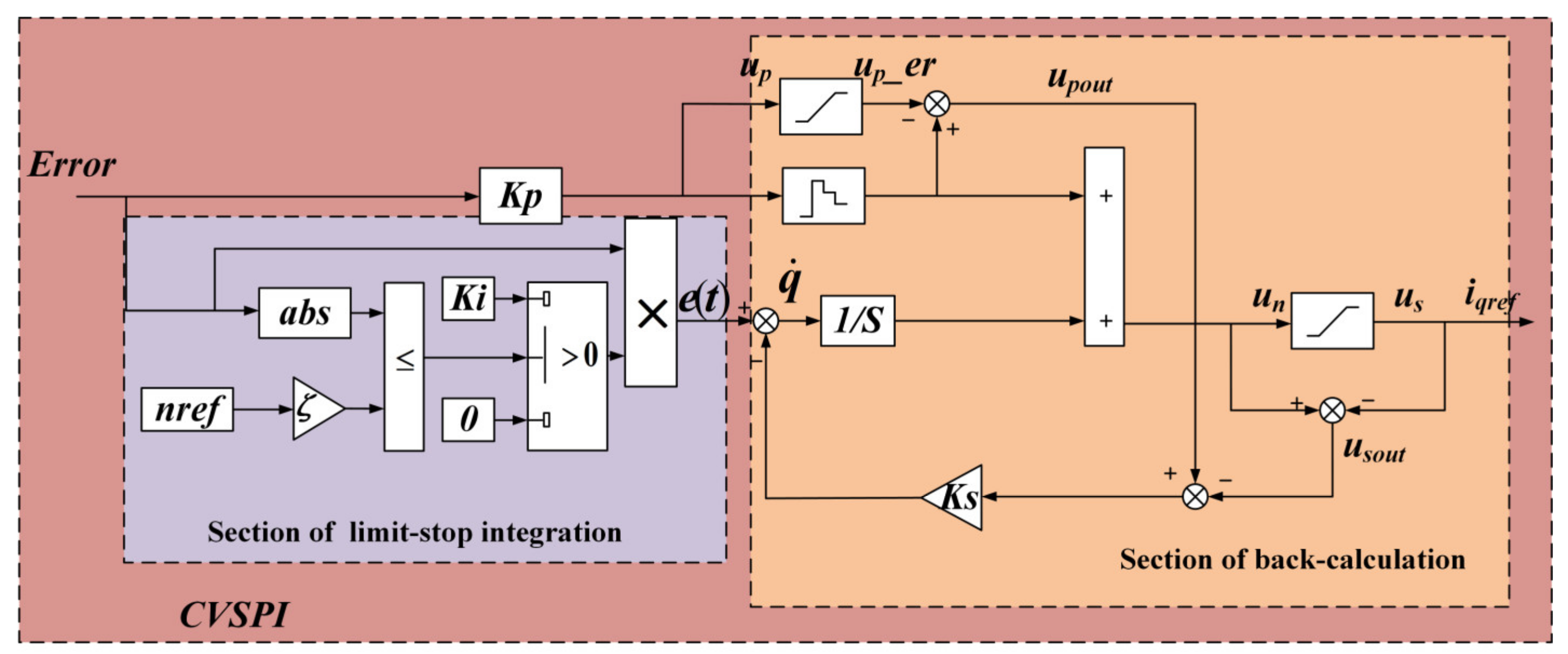
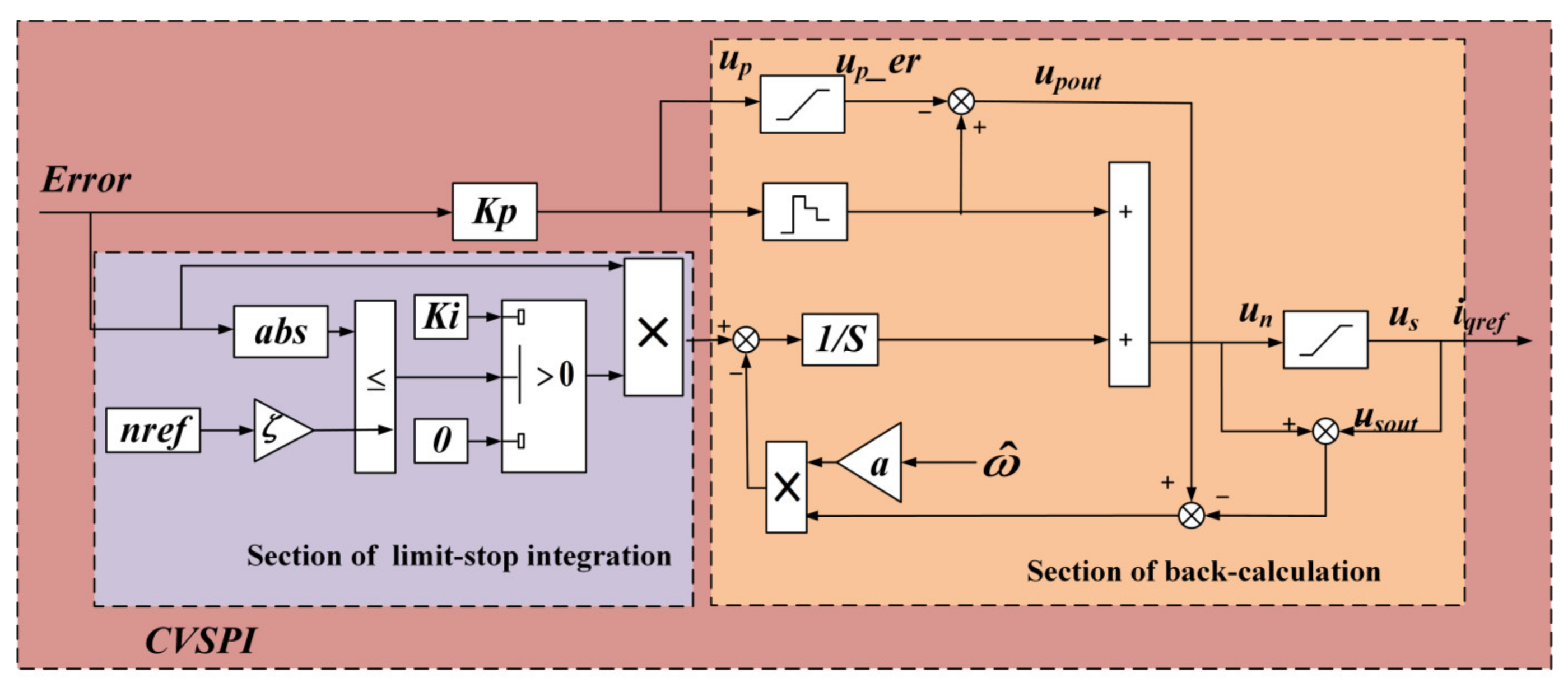
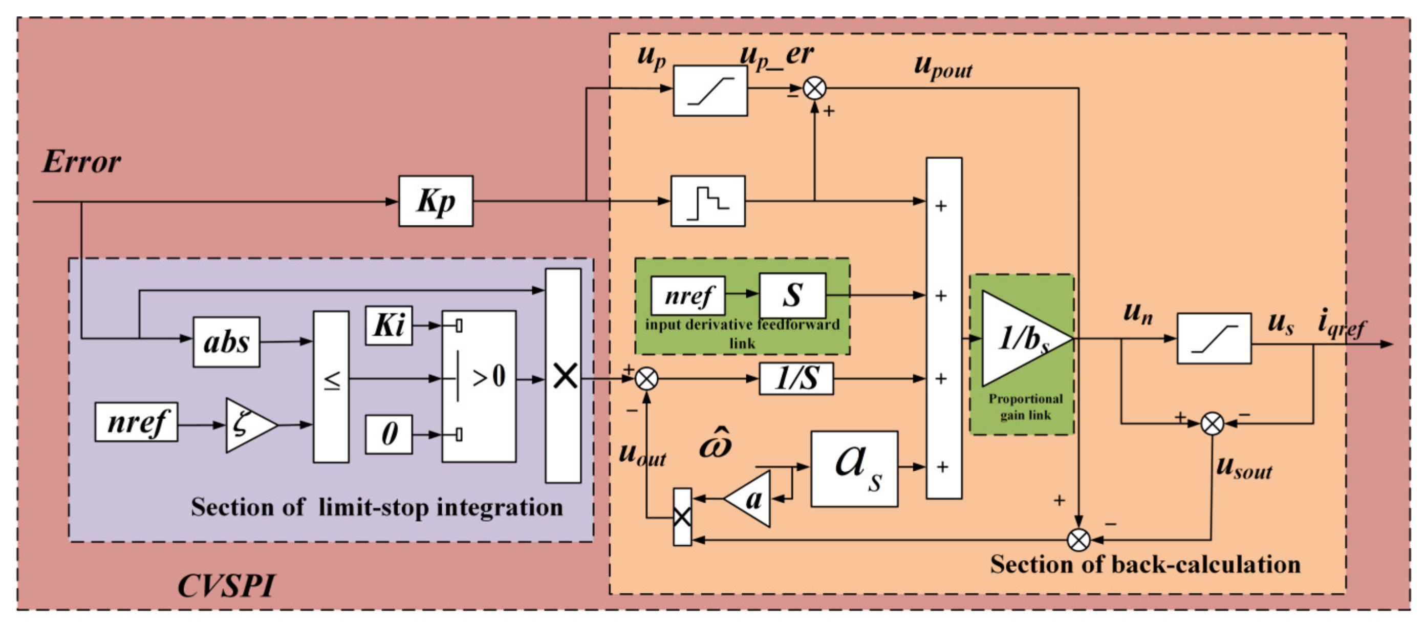
2.1. Design of the Composite Variable Structure PI

The two main anti-windup control methods are limit-stop integration and back-calculation. The former starts with the nature of the Windup phenomenon in the integration term and chooses to use the integrator action depending on whether the controller output is limited. When the controller is saturated, the integrator action is canceled, and the controller is equivalent to a P control. In contrast, when the controller output is in the linear region, the integrator action is added to obtain excellent steady-state control performance. However, the generality is poor, and the parameters selected are fixed and challenging to transpose. The latter method reduces the input to the integrator by feeding back the difference between the input and output quantities of the saturated non-linear link to the information of the integrator, thus suppressing the Windup phenomenon. This method has a linear structure, is easy to design, and is a commonly used Anti-Windup control method in engineering today. However, its transient control performance is heavily dependent on the feedback gain rather than the parameters of the PI controller. There is hysteresis, making it difficult to achieve the performance targets of a wide range of motor speed control systems in practice.

To improve the control performance of the speed control system, this paper integrates the advantages of the limit stop integral method and the back-calculation method and proposes the CVSPI controller shown in Figure 1. The proportion of the integration coefficient to the regulation time in CVSPI can be automatically adjusted depending on the magnitude of the speed deviation. When there is a large speed deviation (i.e., beginning with the motor’s maximum acceleration), only the proportional term is used to enter the saturation state; and the integral term is allowed to be added to eliminate the residual difference when the speed error is small (which can be adjusted according to the actual situation). This allows the controller to desaturate early, reducing the overshoot of the response speed, reducing the regulation time, and improving the dynamic response and immunity of the system. The CVSPI enhances the system’s dynamic performance based on a simple structure, ensures the control accuracy of the system, enhances the tracking response performance, immunity, and stability of the tacho loop system, and reduces the static and dynamic errors of the system.

To address the problem of low accuracy compensation by the integral term alone, CVSPI treats the compensation of the proportional and integral terms separately, significantly reducing the mutual influence of the proportional and integral terms on saturation. This allows the proportional term to be used to its full potential while also enabling Windup suppression, with few changes to the control structure, making it easy to apply. It is possible to achieve a faster and overshoot-free given time while reducing the impact of the Windup phenomenon on system performance. The integration state can be expressed as follows: $\dot{q}=e(t)-K_s(u_{pout}-u_{sout})$, where $K_s$ is the anti-saturation gain.

According to the above equation, selecting the anti-saturation gain is one of the keys to improving system performance. In previous designs, the anti-saturation gain was determined whether the controller output was saturated or not. This method can improve the dynamic system performance at step response, but a fixed anti-saturation gain cannot better suppress the integral saturation at different given speeds. To obtain the output current out of the saturation state quickly while still being able to respond promptly to changes in the given speed and adapt to different given rates, it is necessary to combine the operating characteristics of the IPMSM in other states using the inverse calculation idea and introducing the estimated rate of MRAS to automatically adjust the anti-saturation gain. Because of this, the anti-saturation gain is built as Equation (1), and its value is set by the motor’s specified speed range. Therefore, the block diagram of the CVSPI controller structure with the addition of variable saturation gain is shown in Figure 2.

$$K_s=a\widehat{\omega }.$$

(1)

2.2. CVSPI Controller Design Based on State Equations

The expression for the electromagnetic torque of the IPMSM in the $dq$ rotating coordinate system is:

$$T_e=\frac{3}{2}{p}_n\left[{\psi }_f+\left(L_d-L_q\right)i_d\right]i_q.$$

(2)

$L_d$ and $L_q$ represent the stator inductance components in the $d-q$ reference frame. $p_n$ is the Pole-pairs number.

The IPMSM mechanical equation of motion is:

$$J\frac{d\mathsf{\Omega }}{dt}=T_e-T_L-B_a\mathsf{\Omega }.$$

(3)

where $T_e$ and $T_L$ are the motor output electromagnetic torque and load torque, respectively;

• $\Omega$ is the rotor mechanical angular speed;
• $J$ is the rotational inertia;
• $B_a$ is the viscous friction factor.

In order to facilitate the analysis of the equation of state for the mechanical angular velocity of the IPMSM, this paper uses vector control with $i_d=0$. This is then obtained from Equation (2):

$$T_e=\frac{3}{2}{p}_n{\psi }_f{i}_q.$$

(4)

Substituting Equation (4) into Equation (3) gives the equation of state for the mechanical angular velocity:

$$\begin{array}{cc}\hfill \dot{\Omega }& =-\frac{B_a}{J}\Omega +\frac{1.5p_n{\psi }_f}{J}{i}_q-\frac{T_L}{J}=-\frac{B_a}{J}\Omega +\frac{K_t}{J}\left(i_q^{\ast }-i_q^{\ast }+i_q\right)-\frac{T_L}{J}\hfill \\ \hfill & =-\frac{B_a}{J}\Omega +\frac{K_t}{J}{i}_q^{\ast }-\frac{K_t\left(i_q^{\ast }-i_q\right)+T_L}{J}=-\frac{B_a}{J}\Omega +\frac{K_t}{J}{i}_q^{\ast }-\frac{T_d}{J}\hfill \\ \hfill & =-a_s\mathsf{\Omega }+b_s{i}_q^{\ast }+d_s(t)\hfill \end{array}.$$

(5)

where the state factor $a_s=B_a/J$; the control gain $b_s=K_t/J$; $i_q{}^{*}$ is the given value of the cross-axis current; the total disturbance torque $T_d=K_t\left(i_q{}^{\ast }-i_q\right)+T_L$, consisting of the disturbance torque due to the current tracking error and the load torque; $K_t$ is the electromagnetic torque factor, $K_t=1.5p_n{\psi }_f$; the disturbance term $d_s(t)=-T_d/J$.

Defining the mechanical angular velocity tracking error $e_s={\mathsf{\Omega }}^{\ast }-\mathsf{\Omega }$, ${\Omega }^{*}$ is the given signal for the mechanical angular velocity of the rotor, the equation of state for the angular velocity tracking error can be obtained as:

$${\dot{e}}_s={\dot{\mathsf{\Omega }}}^{\ast }-\dot{\mathsf{\Omega }}={\dot{\mathsf{\Omega }}}^{\ast }+a_s\mathsf{\Omega }-b_s{i}_q^{\ast }-d_s(t).$$

(6)

Commonly load disturbances cannot be measured, so a linear proportional feedback control law is required, i.e.,:

$${\dot{e}}_s=-k_p{e}_s.$$

(7)

Combining Equations (6) and (7) gives the given signal for the output torque current as:

$$i_q^{\ast }=\frac{{\dot{\mathsf{\Omega }}}^{\ast }+k_p\left({\mathsf{\Omega }}^{\ast }-\mathsf{\Omega }\right)-d_s(t)}{b_s}+\frac{B_a}{1.5p_n{\psi }_f}\Omega .$$

(8)

By introducing an integral term to counteract the effect of the disturbance term $d(t)$ on the system, the given signal for the output torque current of the speed loop under the PI controller is obtained as:

$$i_q^{\ast }=\frac{1}{b_s}\left[{\dot{\mathsf{\Omega }}}^{\ast }+k_p\left({\mathsf{\Omega }}^{\ast }-\Omega \right)+k_i\int \left({\mathsf{\Omega }}^{\ast }-\Omega \right)dt\right]+\frac{B_a}{1.5p_n{\psi }_f}\Omega .$$

(9)

where $k_p$ is the scale factor of the controller, and $k_i$ is the integration factor of the controller.

Therefore, this paper adds an input derivative feed-forward link and a control gain link for a given signal to the CVSPI controller described above. The addition of the input derivative feed-forward and control gain links allows the estimated speed to respond accurately to a continuously varying given signal. A block diagram of the final CVSPI controller proposed in this paper is shown in Figure 3.

When $error>\zeta nref$,

$$u_n=\frac{1}{b_s}(error\cdot k_p+\frac{d}{dt}{n}_{ref}+a_s\widehat{\omega }).$$

(10)

where $\widehat{\omega }$ is the estimated speed, $\widehat{\omega }=\frac{30}{\pi }\widehat{\Omega }$; $n_{ref}$ is the given speed; $error=n_{ref}-\widehat{\omega }$.

$$u_s=i_{qsat}.$$

(11)

where $i_{qsat}$ is the maximum output of the controller after limiting.

When $error\le \zeta nref$,

$$u_n=\frac{1}{b_{\mathrm{s}}}(error\cdot k_p+{\displaystyle \int \left[error\cdot k_i-a\widehat{\omega }\left(u_{pout}-u_{sout}\right)\right]}dt+\frac{d}{dt}{n}_{ref}+a_s\widehat{\omega }).$$

(12)

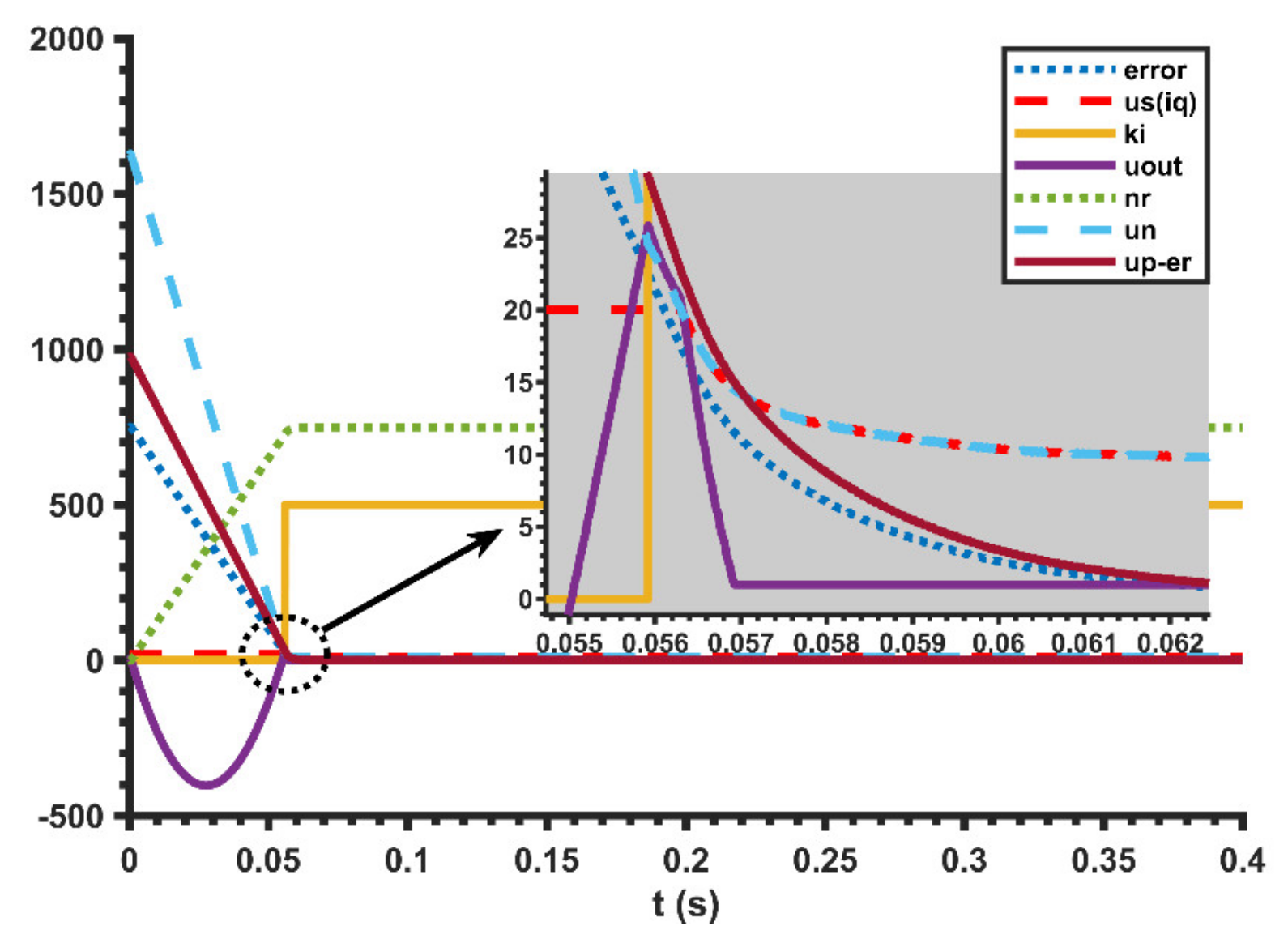
2.3. Performance Analysis of Variable Structure Composite Speed Controllers

Figure 4 shows a comparison of the CVSPI controller outputs for each link when the motor is running at the rated speed with a load of 12 N·m. The mechanical inertia deviation is large at the start, i.e., $error>\zeta nref$. At this point, the integral link does not work and relies on the proportional link to quickly reduce the speed error. At this point, $u_n$ is maximum and $u_s$ is the maximum torque current $i_{qsat}$. This allows the motor to be started up at maximum acceleration. At the same time, the presence of the feedback compensation term ensures that the estimated speed approaches the given speed quickly and without overshooting.

At 0.056 s, the estimated speed reaches 97% of the given speed, at which point $error\le \zeta nref$, the integration link $k_i$ comes into play and is used to eliminate the steady-state error between the estimated speed and the given speed. Since the error is still present, $u_s$ remains at the maximum torque current $i_{qsat}$. At the same time, the anti-integration saturation module performs feedback compensation to suppress system overshoot and oscillation.

At 0.057 s, the estimated speed reaches 99% of the given speed. At this point, $u_s$ is at the desaturation threshold; the feedback compensation term $u_{out}$ is 0. Over the course of 0.057 s ~ 0.062 s, the CVSPI controller changes to a PI controller until the estimated speed reaches the given speed. After the given speed is reached, the system operates stably and accurately with a separate integration link.

The above analysis shows that the CVSPI controller has a different control structure for different error intervals. When the system has a large error, the integral term of the controller does not work, and the output of the controller is clamped at the limiting value to speed up the response. When the error is small, the integral term acts to reduce the steady-state error. At the same time, the anti-saturation gain acts to enable the system to reach a given speed quickly and without overshooting. As the anti-integration saturation gain takes into account the variation in the estimated speed, the CVSPI can be used to achieve accurate, overshoot-free control of the motor in all speed ranges using only a fixed set of parameters. Additionally, the inclusion of an input derivative feed-forward link and a proportional gain link in the CVSPI allows accurate control of the estimated and actual speed even when the given signal is time-varying (e.g., sinusoidal).

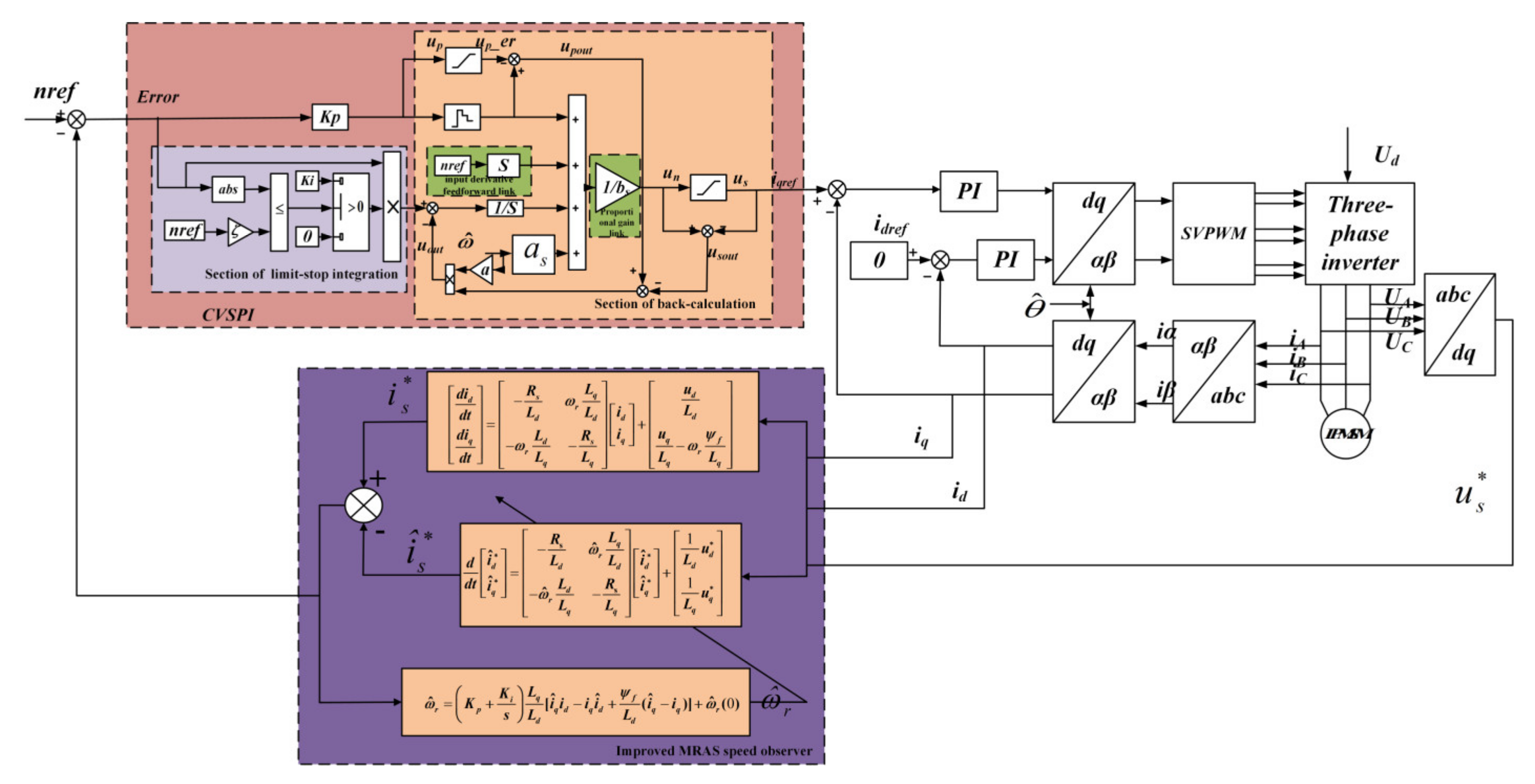
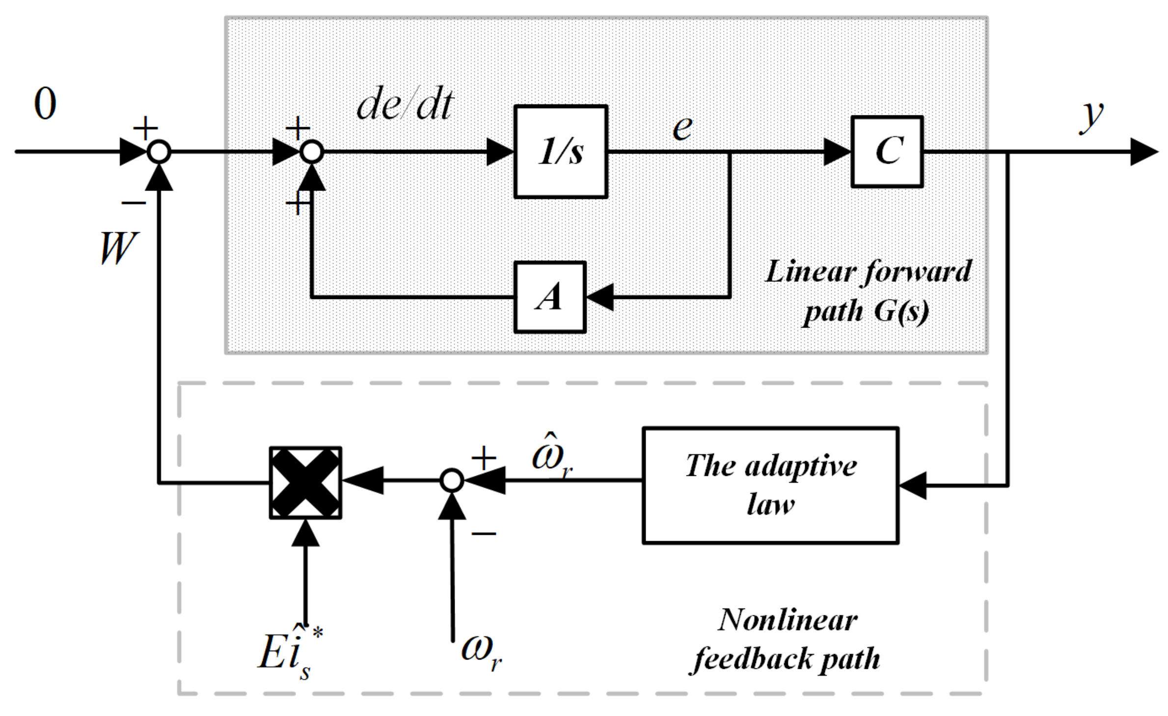
3. Improved MRAS Speed Observer

From the mathematical model of the rotating coordinate system of the built-in permanent magnet synchronous motor:

$$\left[\begin{array}{c}\frac{d{i}_d}{dt}\\ \frac{d{i}_q}{dt}\end{array}\right]=\left[\begin{array}{cc}-\frac{R_s}{L_d}& {\omega }_r\frac{L_q}{L_d}\\ -{\omega }_r\frac{L_d}{L_q}& -\frac{R_s}{L_q}\end{array}\right]\left[\begin{array}{l}{i}_d\hfill \\ i_q\hfill \end{array}\right]+\left[\begin{array}{c}\frac{u_d}{L_d}\\ \frac{u_q}{L_q}-{\omega }_r\frac{{\psi }_f}{L_q}\end{array}\right].$$

(13)

A reference model from the above equation gives:

$$p\left[\begin{array}{c}{i}_d+\frac{{\psi }_f}{L_d}\\ i_q\end{array}\right]=\left[\begin{array}{cc}-\frac{R_{\mathrm{s}}}{L_d}& {\omega }_r\frac{L_q}{L_d}\\ -{\omega }_r\frac{L_d}{L_q}& -\frac{R_{\mathrm{s}}}{L_q}\end{array}\right]\left[\begin{array}{c}{i}_d+\frac{{\psi }_f}{L_d}\\ i_q\end{array}\right]+\left[\begin{array}{c}\frac{1}{L_d}{u}_d+\frac{R_{\mathrm{s}}}{L_d^2}{\psi }_f\\ \frac{1}{L_q}{u}_q\end{array}\right].$$

(14)

where $u_d$ and $u_q$ are the stator voltages in the $d-q$ reference frame; $i_d$ and $i_q$ are the stator currents in the $d-q$ reference frame; $R_s$ is the stator resistance; ${\omega }_r$ is the rotor electrical pulsation; $L_d$ and $L_q$ represent the stator inductance components in the $d-q$ reference frame; ${\psi }_f$ is the magnetic flux.

From the Equation (14), it can be deduced that:

$$p\left[\begin{array}{c}{i}_d^{\ast }\\ i_q^{\ast }\end{array}\right]=\left[\begin{array}{cc}-\frac{R_{\mathrm{s}}}{L_d}& {\omega }_r\frac{L_q}{L_d}\\ -{\omega }_r\frac{L_d}{L_q}& -\frac{R_{\mathrm{s}}}{L_q}\end{array}\right]\left[\begin{array}{c}{i}_d^{\ast }\\ i_q^{\ast }\end{array}\right]+\left[\begin{array}{c}\frac{1}{L_d}{u}_d^{\ast }\\ \frac{1}{L_q}{u}_q^{\ast }\end{array}\right].$$

(15)

where $i_d^{\ast }=i_d+\frac{{\psi }_f}{L_d},i_q^{\ast }=i_q,u_d^{\ast }=u_d+\frac{R_{\mathrm{s}}}{L_d}{\psi }_f,u_q^{\ast }=u_q$.

From the Equation (15), it follows that:

$$p{i}_s^{*}=A{i}_s^{*}+Bu.$$

(16)

In replacing the Equation (16), the speed and current in the equation are replaced by the estimated values to obtain the adjustable model:

$$p\left[\begin{array}{c}{\widehat{i}}_d^{\ast }\\ {\widehat{i}}_q^{\ast }\end{array}\right]=\left[\begin{array}{cc}-\frac{R_{\mathrm{s}}}{L_d}& {\widehat{\omega }}_{\mathrm{r}}\frac{L_q}{L_d}\\ -{\widehat{\omega }}_{\mathrm{r}}\frac{L_d}{L_q}& -\frac{R_{\mathrm{s}}}{L_q}\end{array}\right]\left[\begin{array}{c}{\widehat{i}}_d^{\ast }\\ {\widehat{i}}_q^{\ast }\end{array}\right]+\left[\begin{array}{c}\frac{1}{L_d}{u}_d^{\ast }\\ \frac{1}{L_q}{u}_q^{\ast }\end{array}\right].$$

(17)

where ${\widehat{i}}_d^{\ast }={\widehat{i}}_d+\frac{{\psi }_f}{L_d},{\widehat{i}}_q^{\ast }={\widehat{i}}_q,u_d^{\ast }=u_d+\frac{R_{\mathrm{s}}}{L_d}{\psi }_f,u_q^{\ast }=u_q$.

From the Equation (17), it follows that:

$$p{\widehat{i}}_s^{*}=\widehat{A}{\widehat{i}}_s^{*}+Bu.$$

(18)

Defining the error vector:

$$e=i_s{}^{*}-{\widehat{i}}_s{}^{*}.$$

(19)

Subtracting the reference model from the adjustable model gives:

$$p\left[\begin{array}{c}{e}_d\\ e_q\end{array}\right]=\left[\begin{array}{cc}-\frac{R_{\mathrm{s}}}{L_d}& {\omega }_r\frac{L_q}{L_d}\\ -{\omega }_r\frac{L_d}{L_q}& -\frac{R_{\mathrm{s}}}{L_q}\end{array}\right]\left[\begin{array}{c}{e}_d\\ e_q\end{array}\right]+({\omega }_r-{\widehat{\omega }}_r)\left[\begin{array}{cc}0& \frac{L_q}{L_d}\\ -\frac{L_d}{L_q}& 0\end{array}\right]\left[\begin{array}{c}{\widehat{i}}_d^{\ast }\\ {\widehat{i}}_q^{\ast }\end{array}\right].$$

(20)

From the Equation (20), it follows that:

$$pe=Ae-({\omega }_r-{\widehat{\omega }}_r)J{\widehat{i}}^{*}{}_s=Ae-W.$$

(21)

where $W=({\omega }_r-{\widehat{\omega }}_r)J{\widehat{i}}^{*},A=\left[\begin{array}{cc}-\frac{R_{\mathrm{s}}}{L_d}& {\omega }_r\frac{L_q}{L_d}\\ -{\omega }_r\frac{L_d}{L_q}& -\frac{R_{\mathrm{s}}}{L_q}\end{array}\right],J=\left[\begin{array}{cc}0& \frac{L_q}{L_d}\\ -\frac{L_d}{L_q}& 0\end{array}\right]$.

The Equation (21) describes a standard non-linear time-varying feedback closed-loop system, applicable to Popov’s superstability theory. It consists of a linear constant forward path and a time-varying feedback path. This is seen in Figure 5.

To study the stability of the system shown in Figure 5, assume that $r(t)=0$, then we have $u(t)=-w(t)$, then the forward pathway can be described as [27]:

$$\left\{\begin{array}{l}\dot{x}(t)=Ax(t)+Bu(t)=Ax(t)-Bw(t)\hfill \\ y(t)=Cx(t)+Du(t)=Cx(t)-Dw(t)\hfill \end{array}\right..$$

(22)

The feedback path is:

$$w(t)=\psi [y(t),t,\tau ].$$

(23)

where $x(t)$ is the state variable; $u(t)$ and $y(t)$ are the input and output variables respectively; $A$ is the system matrix; $B$ is the input matrix; $C$ is the output matrix; $D$ is the direct transfer matrix. The forward path selects the matrix $C$ to ensure the system’s stability. According to Popov’s theorem, the system matrix is given by Equations (22) and (23). The sufficient conditions for a system to be asymptotically super-stable are [28]:

1.

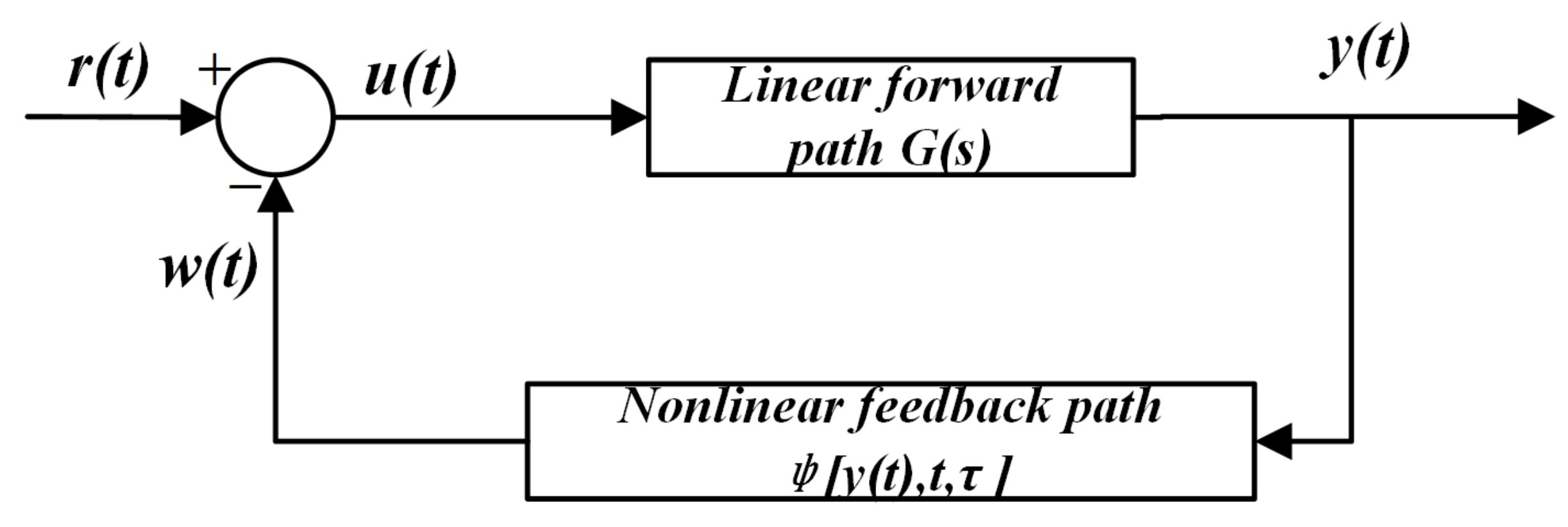
The transfer function matrix $G(s)$ of the forward path is strictly orthogonal, i.e.,:

$$G(s)=D+C{(sI-A)}^{-1}B.$$

(24)

2.

The inputs $y(t)$ and outputs $w(t)$ of the feedback path satisfy Popov’s inequality:

$$\eta (0,t_1)={\displaystyle {\int }_0^{t_1}{W}^T}ydt\ge -r_0{}^2(\forall t_1>0,r_0{}^2\ge 0).$$

(25)

Consequently, the error system derived from the Equation (21) can be represented as an equation of state using the Equation (22):

$$\left\{\begin{array}{l}pe=Ae-W\hfill \\ y=Ce\hfill \end{array}\right.$$

(26)

According to the Equation (26), a block diagram of the structure of the error system in Figure 6 is obtained. The solid line is a linear time-invariant (LTI) system. Since the relationship between the output quantity $y$ and the feedback quantity $W$ is uncertain, a non-linear time-varying feedback system (LTV) is used here to represent their relationship.

For the system shown above to be asymptotically stable, it is necessary to satisfy both Equations (24) and (25). For a conventional MRAS, the linear compensation matrix $C$ is set to the unit matrix $E$. The adaptive law must be redesigned to achieve better speed discrimination over a broad domain.

3.1. Selection of the Linear Compensator Matrix C

The sufficient and necessary conditions for the transfer function matrix $G(s)$ shown in the Equation (24) to be a strictly positive real matrix are that there are symmetric positive definite matrices $P$, $Q$ and real number matrices $K$, $L$, and positive actual number $\lambda$, which satisfy:

$$\left\{\begin{array}{l}PA+A^{T}P=-L{L}^T-2\lambda P=-Q\hfill \\ B^{T}P+K^T{L}^T=C\hfill \\ K^{T}K=D+D^T\hfill \end{array}\right..$$

(27)

The Equation (21) shows that the $B$ matrix is equal to the unit array, and the $D$ matrix is similar to the zero matrices.

Consequently, the Equation (27) can be reduced to:

$$\left\{\begin{array}{l}PA+A^{T}P=-Q\hfill \\ P=C\hfill \end{array}\right..$$

(28)

Therefore, $G(s)$ is strictly positive if a reasonable positive definite compensation matrix $C$ is chosen, so that $P$ and $Q$ are positive definite matrices.

Set up: $P=\left[\begin{array}{cc}{a}_{11}& a_{12}\\ a_{21}& a_{22}\end{array}\right],Q=\left[\begin{array}{cc}{b}_{11}& b_{12}\\ b_{21}& b_{22}\end{array}\right]$, where $a_{12}=a_{21}$, $b_{12}=b_{21}$. By substituting $P$ and $Q$ into the Equation (28):

$$\begin{array}{l}-Q=PA+A^{T}P=\\ \left[\begin{array}{cc}-2a_{11}\frac{R_{\mathrm{s}}}{L_d}-2a_{12}{\omega }_r\frac{L_d}{L_q}& a_{11}{\omega }_{\mathrm{r}}\frac{L_q}{L_d}-a_{12}(\frac{R_{\mathrm{s}}}{L_q}+\frac{R_{\mathrm{s}}}{L_d})-a_{22}{\omega }_r\frac{L_d}{L_q}\\ a_{11}{\omega }_r\frac{L_q}{L_d}-a_{21}(\frac{R_{\mathrm{s}}}{L_q}+\frac{R_{\mathrm{s}}}{L_d})-a_{22}{\omega }_r\frac{L_d}{L_q}& -2a_{22}\frac{R_{\mathrm{s}}}{L_q}+2a_{12}{\omega }_r\frac{L_q}{L_d}\end{array}\right]\end{array}$$

(29)

Prove the positivity of $Q$ using the trace and determinant of the matrix. The following equation needs to be satisfied:

$$\left\{\begin{array}{c}tr(Q)=b_{11}+b_{22}>0\\ \det (Q)=b_{11}{b}_{22}-b_{12}{b}_{21}>0\end{array}\right..$$

(30)

I assume that the new matrix $C$ is: $a_{12}=a_{21}=0,a_{11}=1,a_{22}=\frac{L_q{}^2}{L_d{}^2}$.

The Equation (29) can be reduced to:

$$-Q=\left[\begin{array}{cc}-2\frac{R_{\mathrm{s}}}{L_d}& 0\\ 0& -2\frac{L_q}{L_d{}^2}{R}_s\end{array}\right].$$

(31)

Therefore,

$$\left\{\begin{array}{c}tr(Q)=2\ast \frac{R_{\mathrm{s}}}{L_d}+2\ast \frac{L_q}{L_d{}^2}\ast R_s\\ \det (Q)=2\ast \frac{R_{\mathrm{s}}}{L_d}\ast 2\ast \frac{L_q}{L_d{}^2}\ast R_s\end{array}\right..$$

(32)

Clearly, $tr(Q)$ is greater than zero and $\det (Q)$ is greater than zero. So $Q$ is an integer matrix.

Therefore, take:

$$C=P=\left[\begin{array}{cc}1& 0\\ 0& \frac{L_q{}^2}{L_d{}^2}\end{array}\right].$$

(33)

This guarantees the strict validity of $G(s)$.

3.2. Design of the Adaptive Law

Substituting $y=Ce$ and $W=({\widehat{\omega }}_r-{\omega }_r)J{\widehat{i}}^{*}$ into

$\eta (0,t_1)={\displaystyle {\int }_0^{t_1}{W}^T}ydt\ge -r_0{}^2(\forall t_1>0)$ gives:

$$\eta (0,t_1)={\displaystyle {\int }_0^{t_1}({\widehat{\omega }}_r-{\omega }_r){(J{\widehat{i}}^{*})}^T}\ast Cedt.$$

(34)

MRAS parameters are estimated using a proportional integral form, denoted ${\widehat{\omega }}_r$ as:

$${\widehat{\omega }}_r={\displaystyle {\int }_0^t{F}_1(y,t,\tau )d\tau +F_2(y,t)+{\widehat{\omega }}_r(0)}.$$

(35)

where ${\widehat{\omega }}_r(0)$ is the initial value.

Substitute Equation (36) into Equation (35) to obtain:

$$\begin{array}{cc}\hfill & \eta \left(0,t_1\right)={\int }_0^{t_1}\left[{\int }_0^t{F}_1(y,t,\tau )d\tau +{\widehat{\omega }}_r\left(0\right)-{\omega }_r\right]{\left(J{\widehat{i}}_s^{*}\right)}^{T}Cedt+\hfill \\ \hfill & {\int }_0^{t_1}{F}_2(y,t){\left(Jy{\widehat{i}}_s^{*}\right)}^{T}Cedt={\eta }_1\left(0,t_1\right)+{\eta }_2\left(0,t_1\right)\hfill \end{array}$$

(36)

To satisfy $\eta (0,t_1)={\displaystyle {\int }_0^{t_1}{W}^T}ydt\ge -r_0{}^2(\forall t_1>0,r_0{}^2\ge 0)$, it is possible to make respectively:

$${\eta }_1\left(0,t_1\right)\ge -r_1{}^2(r_1\ge 0).$$

(37)

$${\eta }_2\left(0,t_1\right)\ge -r_2{}^2(r_2\ge 0).$$

(38)

For the inequality (37), construct a function $f(t)$ satisfying:

$$\left\{\begin{array}{c}\frac{d}{dt}f\left(t\right)={\left(J{{\widehat{i}}^{*}}_s\right)}^{T}Ce\\ kf\left(t\right)={\int }_0^t{F}_1(y,t,\tau )d\tau +{\widehat{\omega }}_r\left(0\right)-{\omega }_r\end{array}\right.$$

(39)

where $k>0$. Substituting Equation (40) into Equation (38) gives:

$${\eta }_1\left(0,t_1\right)={\int }_0^{t_1}kf\left(t\right)\frac{df\left(t\right)}{dt}dt=\frac{k}{2}\left[f^2\left(t_1\right)-f^2\left(0\right)\right]\ge -\frac{k}{2}{f}^2\left(0\right)\ge -r_1^2$$

(40)

The derivative of the Equation (40) is:

$$k\frac{d}{dt}f(t)=F_1(y,t,\tau ).$$

(41)

Substitute Equation (39) into Equation (41) yields:

$$F_1(y,t,\tau )=K_i{\left(J{\widehat{i}}_s{}^{*}\right)}^{T}Ce\hspace{1em}(K_i>0).$$

(42)

For the Equation (38), the inequality must hold if the product function is positive, so take:

$$F_2(y,t)=K_p{\left(J{\widehat{i}}_s{}^{*}\right)}^{T}Ce\hspace{1em}(K_p>0).$$

(43)

Substitute Equation (43) into Equation (38) yields:

$${\eta }_2\left(0,t_1\right)={\int }_0^{t_1}{K}_p{\left(J{{\widehat{i}}_s}^{*}\right)}^{T}Ce{\left(J{{\widehat{i}}_s}^{*}\right)}^{T}Cedt\ge 0\ge -r_2^2$$

(44)

Combining Equations (41) and (45) into Equation (36) yields:

$${\widehat{\omega }}_r={\int }_0^t{K}_i{\left(J{{\widehat{i}}_s}^{*}\right)}^{T}Cedt+K_p{\left(J{{\widehat{i}}_s}^{*}\right)}^{T}Ce+{\widehat{\omega }}_r\left(0\right)$$

(45)

where

$$\begin{array}{l}{\left(J{\widehat{i}}_s{}^{*}\right)}^{T}Ce={({\widehat{i}}_s{}^{*})}^T{J}^{T}Ce\\ =\left[\begin{array}{cc}{\widehat{i}}_d{}^{*}& {\widehat{i}}_q{}^{*}\end{array}\right]\left[\begin{array}{cc}0& -\frac{L_d}{L_q}\\ \frac{L_q}{L_d}& 0\end{array}\right]\left[\begin{array}{cc}1& 0\\ 0& \frac{L_q{}^2}{L_d{}^2}\end{array}\right]\left[\begin{array}{c}{i}_d^{*}-{\widehat{i}}_d{}^{*}\\ i_q^{*}-{\widehat{i}}_q{}^{*}\end{array}\right]=\frac{L_q}{L_d}[{\widehat{i}}_q{i}_d-i_q{\widehat{i}}_d+\frac{{\psi }_f}{L_d}({\widehat{i}}_q-i_q)]\end{array}$$

(46)

Therefore, the new speed adaptive law is derived as follows:

$${\widehat{\omega }}_r=\left(K_p+\frac{K_i}{s}\right)·\frac{L_q}{L_d}[{\widehat{i}}_q{i}_d-i_q{\widehat{i}}_d+\frac{{\psi }_f}{L_d}({\widehat{i}}_q-i_q)]+{\widehat{\omega }}_r(0).$$

(47)

In summary, the structure of the IPMSM speed control-free speed regulation system is shown in Figure 7.

4. Simulation Results and Analysis

The estimated speed of the MRAS observer proposed in the text is introduced into the system feedback, and an IPMSM simulation platform is built to verify the speed loop control strategy proposed in this paper, demonstrating the high performance of the velocity-free variable frequency speed control system under CVSPI controller (nref is the given speed, nr is the estimated MRAS speed, and nw is the response speed). The parameters of the IPMSM used in the simulation are shown in

Table 1. IPMSM parameters.

Parameters	Value
$\mathrm{Rated} \mathrm{torque} T/\left(\mathrm{N}\cdot \mathrm{m}\right)$	25
$\mathrm{Rated} \mathrm{speed} {\omega }_{ref}\left(\mathrm{r}/\min \right)$	750
$\mathrm{Stator} \mathrm{resistance} R_s/\Omega$	2.875
$\mathrm{Cross}-\mathrm{axis} \mathrm{inductance} L_q/\mathrm{mH}$	8.5
$\mathrm{Straight}-\mathrm{axis} \mathrm{inductance} L_d/\mathrm{mH}$	8.0
$\mathrm{Magnetic} \mathrm{flux} {\psi }_f/\mathrm{wb}$	0.175
$\mathrm{Pole}-\mathrm{pairs} \mathrm{number} p_n$	4
$\mathrm{Rotational} \mathrm{inertia} J/\left(\mathrm{kg}\cdot {\mathrm{m}}^2 \right)$	0.008

.

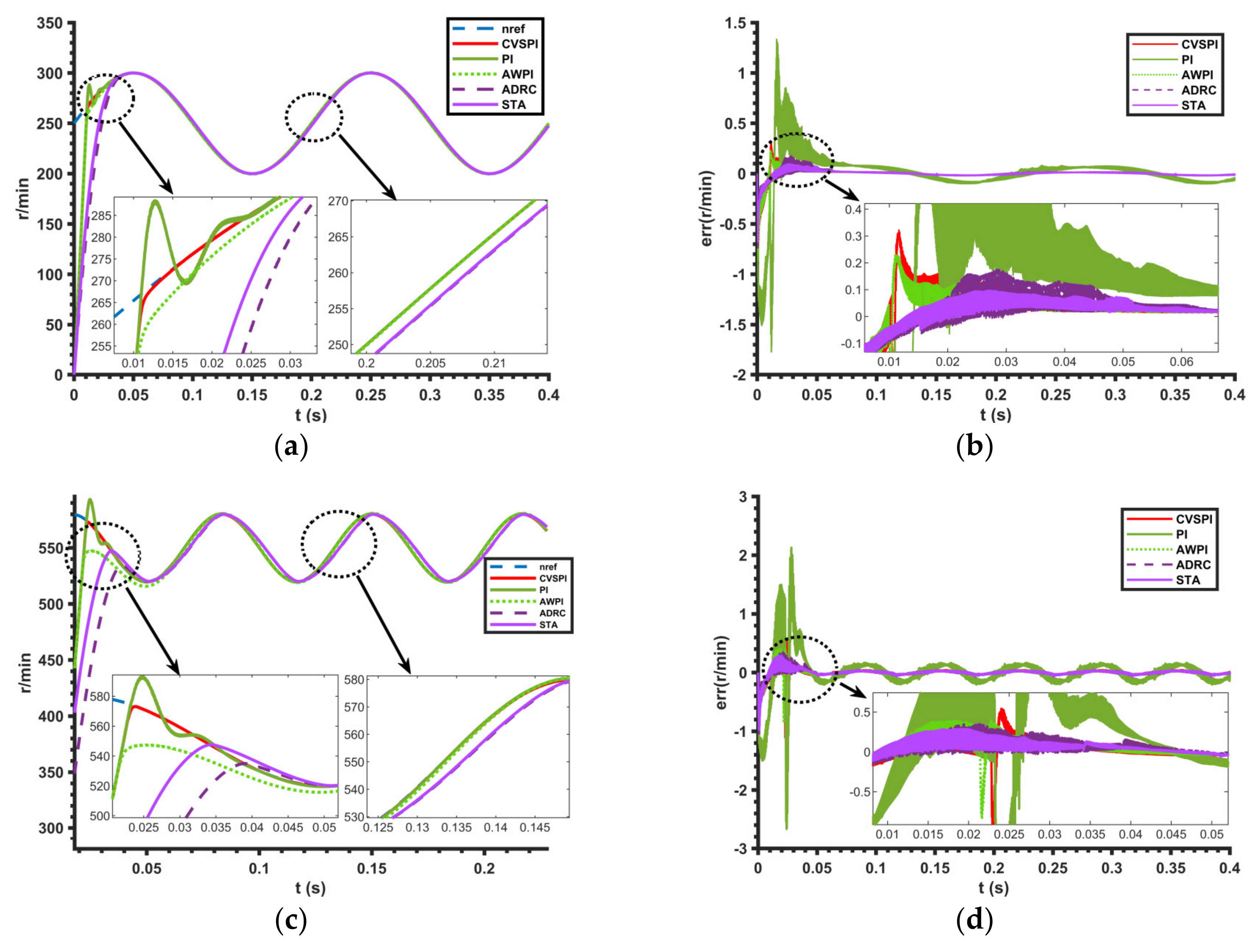
4.1. Test of System Dynamic Followership

CVSPI control is compared with the conventional PI controller, anti-windup PI (AWPI) controller proposed in the literature [27], active disturbance rejection controller (ADRC) proposed in the literature [20], and Super-twisting algorithm (STA) proposed in the literature [25] to verify the advantages of the system speed tracking response performance under CVSPI control. nw under five-speed controllers given by sinusoidal speed is shown in Figure 8a,c, and the error of nr vs. nw is shown in Figure 8b,d, where the given sine speed is divided into two cases: (i) the peak is 300 r/min, the trough is 200 r/min, and the frequency is 5 Hz; (ii) the peak is 580 r/min, the trough is 520 r/min, and the frequency is 15 Hz. When the given sine speed is the first scenario, as shown in Figure 8a,b, the performance comparison is shown in

Table 2. Performance comparison with a peak of 300 r/min, a trough of 200 r/min, and a frequency of 5 hz.

Control Strategies	CVSPI	PI	AWPI	ADRC	STA	Unit
Response time	0.01	0.02	0.026	0.026	0.028	s
Start overshoot	0	7.69%	0	0	0
The error between the actual speed and the estimated speed	±0.6	±2.0	±1.5	±0.8	±0.8	r/min
The steady-state error between the given speed and the estimated speed	±0.01	±0.1	±2	±5.2	±5	r/min

.

Similarly, when the given sine speed is the second case, as shown in Figure 8c,d, the performance comparison is shown in

Table 3. Performance comparison with a peak of 580 r/min and a trough of 520 r/min at 15 hz.

Control Strategies	CVSPI	PI	AWPI	ADRC	STA	Unit
Response time	0.02	0.04	0.042	0.05	0.05	s
Start overshoot	0	5.67%	0	0	0
The error between the actual speed and the estimated speed	±0.6	±2.0	±1.5	±0.8	±0.8	r/min
The steady-state error between the given speed and the estimated speed	±0.01	±0.1	±2	±10	±10	r/min

.

As can be seen from Figure 8a,d and Table 2 and Table 3, the CVSPI has no overshoot, has the shortest regulation time and the smallest steady-state error for a given sinusoidal signal, and also minimizes the error between estimated and actual speed compared to the PI, AWPI, ADRC, and STA. the PI has a large overshoot. At larger bandwidths, ADRC and STA have larger steady-state errors.

The CVSPI controller can be proven to respond faster and more accurately to a given system signal, effectively increasing the response bandwidth of the system’s speed loop while also providing better dynamic characteristics.

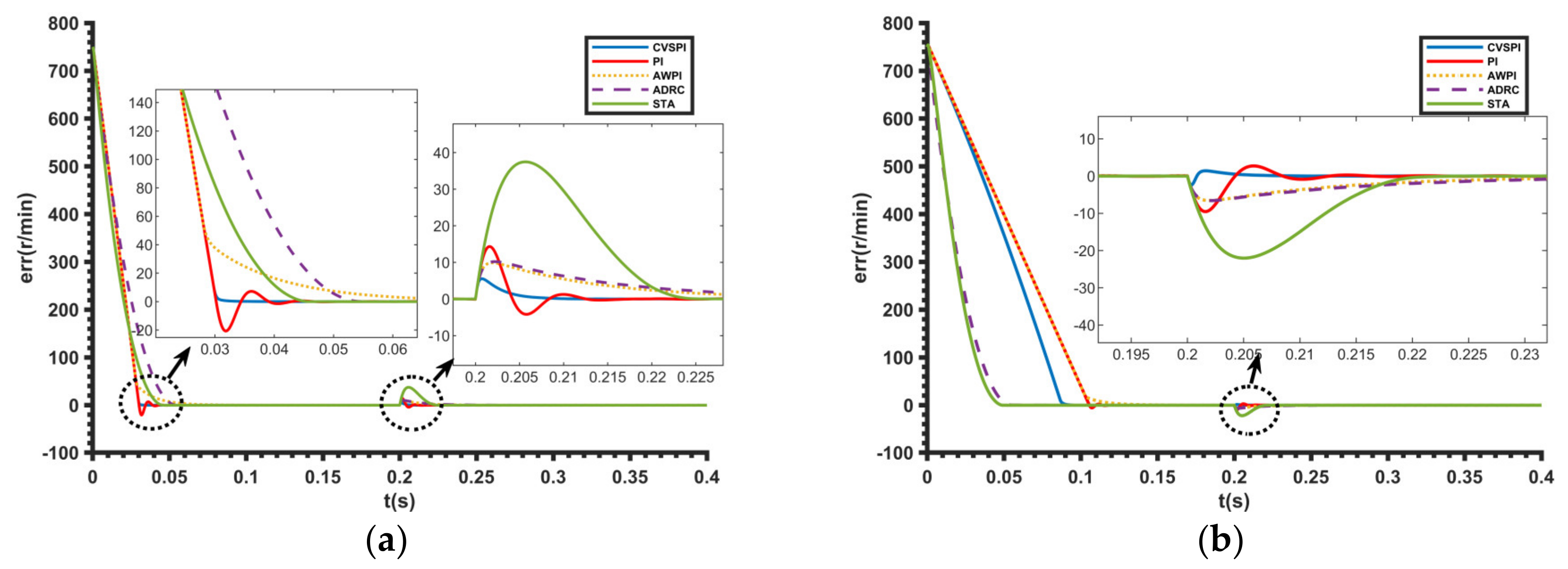
4.2. Evaluation of System Immunity

By adding and withdrawing loads suddenly at rated speed, we compared the nw of the CVSPI controller to that of the PI controller, AWPI, ADRC, and STA, validating the advantages of the CVSPI controller in terms of resistance to external load disturbance performance. Figure 9a shows the error of nref versus nr for the five-speed controllers at 0.2 s with a sudden 15 N·m load. The performance comparison is shown in

Table 4. Comparison of performance at 0.2 s with a sudden 15 N·m load at rated speed.

Control Strategies	CVSPI	PI	AWPI	ADRC	STA	Unit
Response time	0.03	0.05	0.06	0.055	0.04	s
Start overshoot	0	7.69%	0	0	0
Regulation time	10	15	17	20	30	ms
Speed variation under load disturbance	10	20	18	18	40	r/min

.

Figure 9b shows the error of nref versus nr for operation with a load of 15 N·m at rated speed for five-speed controllers, with sudden unloading of the load to 5 N·m at 0.2 s. The performance comparison is shown in

Table 5. Comparison of performance with a load of 15 N·m at rated speed and a sudden load relief of 5 N·m at 0.2 s.

Control Strategies	CVSPI	PI	AWPI	ADRC	STA	Unit
Response time	0.08	0.12	0.12	0.06	0.04	s
Start overshoot	0	2.39%	0	0	0
Regulation time	10	15	18	20	20	ms
Speed variation under load disturbance	8	18	15	15	40	r/min

.

As can be seen from Figure 9a,b and Table 5, the amount of fluctuation in speed response under CVSPI control is about 60% lower than conventional PI control, about 50% lower than AWPI control, about 48% lower than ADRC control and about 70% lower than STA control at the instant of sudden load addition and removal, and the steady-state recovery time is also shorter than that of conventional PI, AWPI, ADRC, and STA control. The steady-state recovery time is also shorter than conventional PI, AWPI, ADRC, and STA control. Although the system takes slightly longer to reach rated speed under CVSPI control than under ADRC and STA at start-up with load, CVSPI control is considerably more resilient to load disturbances than the other controls.

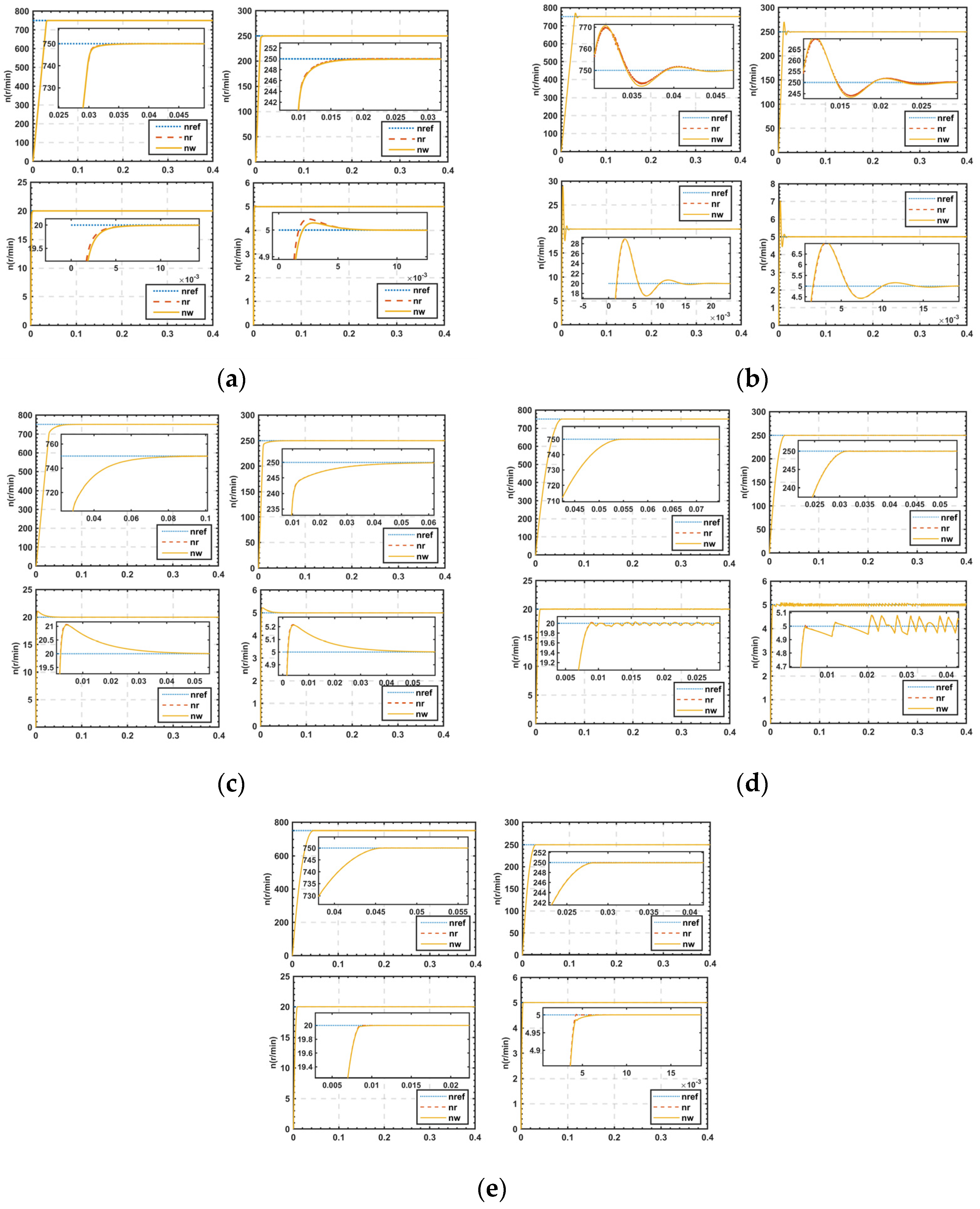
4.3. Evaluation of Systemwide Speed Domain Performance

Under no-load conditions, the high, medium, and low-speed response waveforms and speed estimate waveforms under CVSPI control were compared with the traditional PI, AWPI, ADRC, and STA controller to validate the performance of the CVSPI controller with wide speed domain speed tracking response. The performance of nw and nr for the five-speed controllers at 5 r/min, 15 r/min, 250 r/min, and 750 r/min is shown in Figure 10a–e. The performance comparison is shown in

Table 6. Comparison of performance in the broad speed domain.

Control Strategies	750 r/min	250 r/min	20 r/min	5 r/min
CVSPI	Smooth	Smooth	Smooth	Smooth
PI	Overtones	Overtones	Fluctuations	Fluctuations
AWPI	Smooth	Smooth	Overtones	Overtones
ADRC	Smooth	Smooth	Smooth	Severe chatter
STA	Smooth	Smooth	Smooth	Smooth

.

From Figure 10a–e and Table 6, it can be seen that the conventional PI will show large fluctuations in the speed response at low speed and obvious overshoot at medium and high speed; AWPI can suppress overshoot at high and medium speed better but will show overshoot at low speed; ADRC can respond better to different speed situations at high and low speed but has poor static stability at very low speed (e.g., 5 r/min). STA can achieve accurate speed following at different speeds. The CVSPI control can be proven to be superior to the other four controls in achieving high performance and high accuracy control of the IPMSM and a wide speed range with no static stability and fast performance.

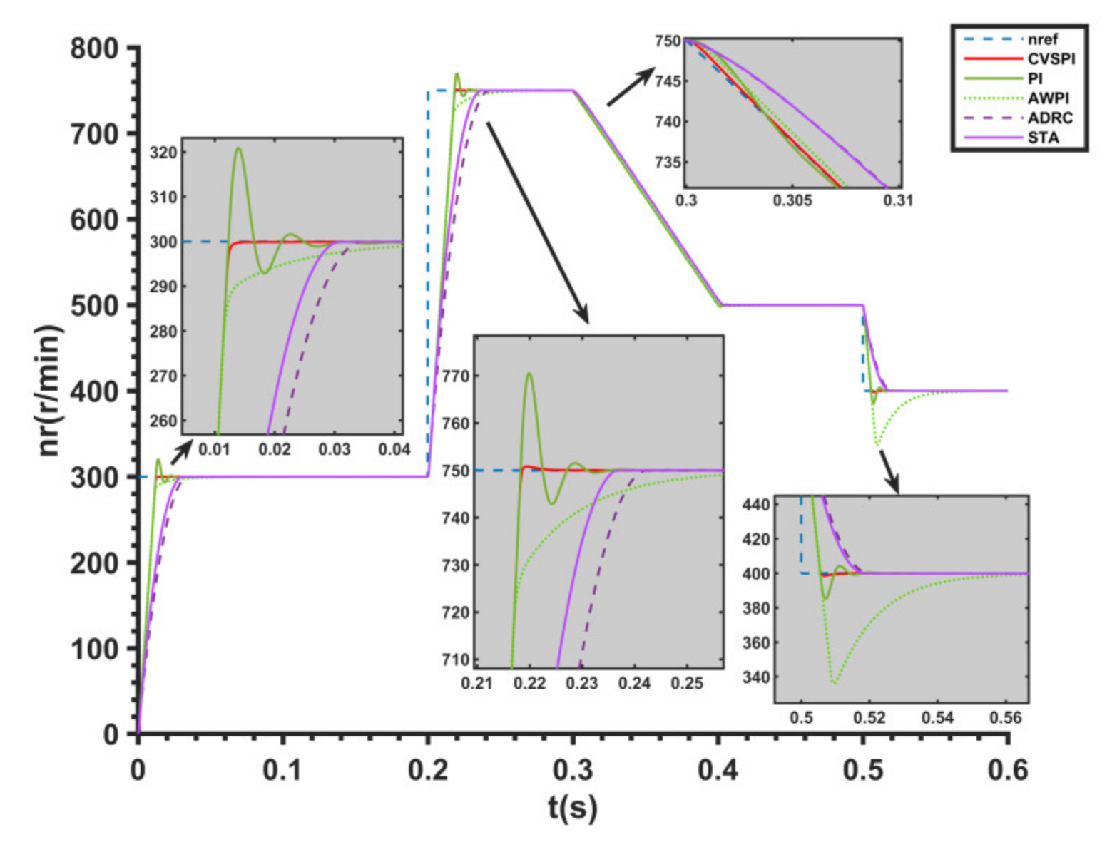
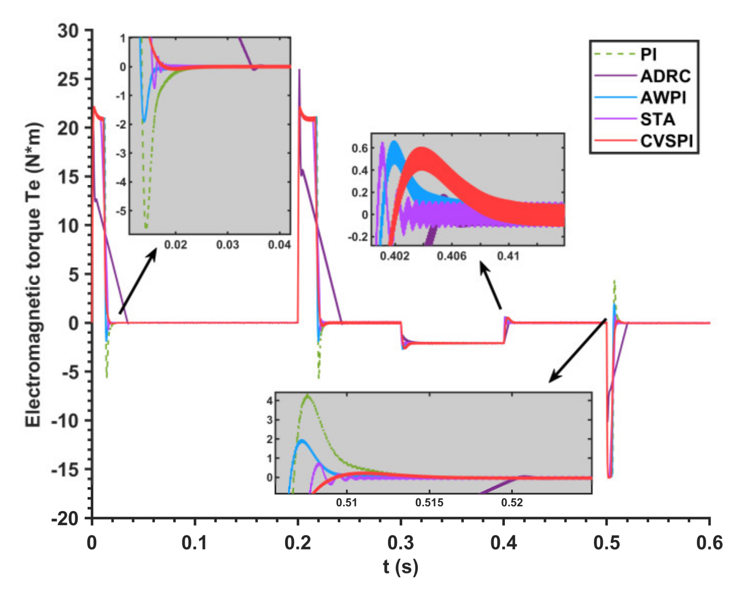
4.4. Analyzing the Effects of a Sudden Change in Speed While Maintaining a Consistent Torque Load

Figure 11 shows the estimated speed waveforms of the system under CVSPI, PI, AWPI, ADRC, and STA control during sudden speed changes. The motor starts at no load and starts at a given speed of 300 r/min, steps to rated speed at 0.2 s, becomes a ramp signal at 0.3 s, drops to 500 r/min, and steps down to 400 r/min at 0.5 s. The performance comparison is shown in

Table 7. Comparison of step and ramp signal performance.

Control Strategies	CVSPI	PI	AWPI	ADRC	STA
Step-up signal	Smooth	Overtones	Smooth	Smooth	Smooth
Step-down signal	Smooth	Overtones	Overtones	Smooth	Smooth
Ramp signal	Accuracy	Accuracy	Accuracy	With steady-state error	With steady-state error

.

As can be seen from Figure 11 and Table 7, under CVSPI control, the estimated speed always follows the given speed strictly. The ADRC and STA controls, on the other hand, have a large static error under ramp signals; the PI control has a significant overshoot under step signals, with a speed response overshoot of 19.8%; and the AWPI has a large overshoot under step-down signals.

Figure 12 shows a comparison of the torque under the different control methods. It is clear that the torque under STA control has a chattering phenomenon. The torque under PI and AWPI control has different degrees of overshoot. The torque response under ADRC control is slower. The torque under CVSPI control is smoother and more stable, and the torque response is faster. In summary, the CVSPI controller given in this paper has better dynamic characteristics.

5. Conclusions

(1)

To minimize or do away with speed overshoot and speed-free control system regulation time, this paper builds on the foundation of the conventional AWPI by integrating the benefits of the encounter limit stop integral method and the inverse calculation method to design a CVSPI controller for use in IPMSM speed-free control systems.

(2)

Using the inverse calculation idea to introduce the MRAS estimated speed into the anti-saturation gain to accurately compensate for the system state, enabling the system to quickly exit the integral saturation zone, suppressing the integral saturation phenomenon, and improving the immunity of the system.

(3)

Adding a feed-forward link for a given input differential to accurately respond to time-varying inputs and enhance the speed loop tracking response performance.

(4)

CVSPI can achieve relatively good dynamic following performance using only one set of traditional PI controller parameters. The parameters are relatively easy to adjust.

(5)

To enable MRAS to operate efficiently over a wide speed range, a new linear compensator was designed, and a new speed adaptive law was derived.

Simulation results verify that CVSPI can achieve high performance, high accuracy control, and wide speed domain static differential-free speed regulation in an IPMSM speed-free control system and solve the overshoot of the step response. The estimated speed under different input signals is closer to the actual motor speed and has better static and dynamic performance. A new approach is provided for the study of high-performance permanent magnet synchronous motor speed control systems without speed sensors.

References

- Zhang, X.; Tao, R.; Xu, X.; Wang, T.; Zhang, H. Predictive Current Control of a PMSM Three-Level Dual-Vector Model Based on Self-Anti-Disturbance Techniques. J. Electr. Eng. Technol 2022, 17, 3375–3388. [Google Scholar] [CrossRef]
- Zhang, L.; Bai, J.; Wu, J. Speed Sensor-Less Control System of Surface-Mounted Permanent Magnet Synchronous Motor Based on Adaptive Feedback Gain Supertwisting Sliding Mode Observer. J. Sens. 2021, 2021, 8301359. [Google Scholar] [CrossRef]
- Wang, F.; Li, J.; Li, Z.; Ke, D.; Du, J.; Garcia, C.; Rodriguez, J. Design of Model Predictive Control Weighting Factors for PMSM Using Gaussian Distribution-Based Particle Swarm Optimization. IEEE Trans. Ind. Electron. 2022, 69, 10935–10946. [Google Scholar] [CrossRef]
- Liu, Q.; Hameyer, K. High-Performance Adaptive Torque Control for an IPMSM With Real-Time MTPA Operation. IEEE Trans. Energy Convers. 2017, 32, 571–581. [Google Scholar] [CrossRef]
- Liu, Y.; Fang, J.; Tan, K.; Huang, B.; He, W. Sliding mode observer with adaptive parameter estimation for sensorless control of IPMSM. Energies 2020, 13, 5991. [Google Scholar] [CrossRef]
- Liu, K.; Hou, C.; Hua, W. A Novel Inertia Identification Method and Its Application in PI Controllers of PMSM Drives. IEEE Access 2019, 7, 13445–13454. [Google Scholar] [CrossRef]
- Hussain, H.A. Tuning and Performance Evaluation of 2DOF PI Current Controllers for PMSM Drives. IEEE Trans. Transp. Electrif. 2021, 7, 1401–1414. [Google Scholar] [CrossRef]
- Kesavan, P.; Karthikeyan, A. Electromagnetic Torque-Based Model Reference Adaptive System Speed Estimator for Sensorless Surface Mount Permanent Magnet Synchronous Motor Drive. IEEE Trans. Ind. Electron. 2020, 67, 5936–5947. [Google Scholar] [CrossRef]
- Khlaief, A.; Boussak, M.; Chaari, A. A MRAS-based stator resistance and speed estimation for sensorless vector controlled IPMSM drive. Electr. Power Syst. Res. 2014, 108, 1–15. [Google Scholar] [CrossRef]
- Savitski, D.; Ivanov, V.; Augsburg, K.; Emmei, T.; Fuse, H.; Fujimoto, H.; Fridman, L.M. Wheel Slip Control for the Electric Vehicle With In-Wheel Motors: Variable Structure and Sliding Mode Methods. IEEE Trans. Ind. Electron. 2019, 99, 8535–8544. [Google Scholar] [CrossRef]
- Tursini, M.; Parasiliti, F.; Zhang, D. Real-time gain tuning of PI controllers for high-performance PMSM drives. IEEE Trans. Ind. Appl. 2002, 38, 1018–1026. [Google Scholar] [CrossRef]
- Nalepa, R. Generic criterion for tuning of adaptive digital PI current compensators of PMSM drives. IEEE Int. Symp. Ind. Electron. 2011, 2011, 601–606. [Google Scholar] [CrossRef]
- Gücin, T.N.; Biberoğlu, M.; Fincan, B.; Gülbahçe, M.O. Tuning cascade PI(D) controllers in PMDC motor drives: A performance comparison for different types of tuning methods. Int. Conf. Electr. Electron. Eng. 2015, 2015, 1061–1066. [Google Scholar] [CrossRef]
- Xiao, X.; Li, Y.; Li, M. Performance control of PMSM drives using a self-tuning PID. IEEE Int. Conf. Electr. Mach. Drives 2005, 2005, 1053–1057. [Google Scholar] [CrossRef]
- Djelamda, I.; Bouchareb, I.; Lebaroud, A. High performance hybrid FOC-fuzzy-PI controller for PMSM drives. Eur. J. Electr. Eng. 2021, 23, 301–310. [Google Scholar] [CrossRef]
- Sarsembayev, B.; Suleimenov, K.; Do, T.D. High Order Disturbance Observer Based PI-PI Control System with Tracking Anti-Windup Technique for Improvement of Transient Performance of PMSM. IEEE Access 2021, 9, 66323–66334. [Google Scholar] [CrossRef]
- Repecho, V.; Waqar, J.; Biel, D.; Doria-Cerezo, A. Zero speed sensorless scheme for PMSM under decoupled sliding mode control. IEEE Trans. Ind. Electron. 2021, 99, 1288–1297. [Google Scholar] [CrossRef]
- Wang, Y.; Xu, Y.; Zou, J. Sliding-Mode Sensorless Control of PMSM With Inverter Nonlinearity Compensation. IEEE Trans. Power Electron. 2019, 2019, 10206–10220. [Google Scholar] [CrossRef]
- Lu, E.; Li, W.; Yang, X.; Liu, Y. Anti-disturbance speed control of low-speed high-torque PMSM based on second-order non-singular terminal sliding mode load observer. ISA Trans. 2018, 88, 142–152. [Google Scholar] [CrossRef]
- Wang, S. ADRC and Feedforward Hybrid Control System of PMSM. Math. Probl. Eng. 2013, 2013, 180179. [Google Scholar] [CrossRef]
- Rong, Z.; Huang, Q. A new PMSM speed modulation system with sliding mode based on active-disturbance-rejection control. J. Cent. South Univ. 2016, 23, 1406. [Google Scholar] [CrossRef]
- Gai, J.; Huang, S.; Huang, Q.; Li, M.; Wang, H.; Luo, D.; Wu, X.; Liao, W. A new fuzzy active-disturbance rejection controller applied in PMSM position servo system. Int. Conf. Electr. Mach. Syst. 2014, 2014, 2055. [Google Scholar] [CrossRef]
- Roy, P.; Roy, B.K. Dual mode adaptive fractional order PI controller with feed-forward controller based on variable parameter model for quadruple tank process. Isa Trans. 2016, 63, 365–376. [Google Scholar] [CrossRef] [PubMed]
- Gao, P.; Zhang, G.; Lv, X. Model-Free Hybrid Control with Intelligent Proportional Integral and Super-Twisting Sliding Mode Control of PMSM Drives. Electronics 2020, 9, 1427. [Google Scholar] [CrossRef]
- Liang, D.; Jian, L.; Qu, R. Super-twisting algorithm based sliding mode observer for wide-speed range PMSM sensorless control considering VSI nonlinearity. In Proceedings of the 2017 IEEE International Electric Machines and Drives Conference (IEMDC), Miami, FL, USA, 21–24 May 2017; pp. 1–7. [Google Scholar] [CrossRef]
- Lee, K.; Ha, J.; Simili, D. Decoupled current control with novel anti-windup for PMSM drives. In Proceedings of the 2017 IEEE Energy Conversion Congress and Exposition (ECCE), Cincinnati, OH, USA, 1–5 October 2017; pp. 1183–1190. [Google Scholar] [CrossRef]
- Yang, M.; Tang, S.; Xu, D. Comments on “Antiwindup Strategy for PI-Type Speed Controller”. IEEE Trans. Ind. Electron. 2015, 62, 1329–1332. [Google Scholar] [CrossRef]
- Turner, M.C.; Sofrony, J.; Prempain, E. Anti-windup for model-reference adaptive control schemes with rate-limits. Syst. Control. Lett. 2020, 137, 104630. [Google Scholar] [CrossRef]