Abstract
Hydroelectric power plants (HEPPs) are renewable energy power plants with the highest installed power in the world. The control systems are responsible for stopping the relevant unit safely in case of any malfunction while ensuring the desired operating point. Conventional control systems detect anomalies at certain limits or predefined threshold values by evaluating analog signals regardless of differences caused by operating conditions. In this study, using real data from a large hydro unit (>150 MW), a normal behavior model of a hydraulic governor’s oil circulation in an operational HEPP is created using several machine learning methods and historical data obtained from the HEPP’s SCADA system. Model outputs resulted in up to 96.45% success of prediction with less than 1% absolute deviation from actual measurements and an R2 score of 0.985 with the random forest regression method. This novel approach makes the model outputs far more appropriate to use as an active threshold value changing for different operating conditions, eliminating insufficiency of the constant threshold, resulting in the detection of anomalies in early stages and taking precautions accordingly. The study fills the gap in the literature on anomaly detection in hydraulic power units, which is a demanding task with state-of-the-art methods.
1. Introduction
Hydroelectric power plants (HEPPs) constitute approximately 40% of renewable energy resources with an installed power of over 3000 GW worldwide. This capacity makes HEPPs have the highest installed capacity in the world among all renewable energy resources [1]. Due to HEPPs’ high share in production, contribution to the operational flexibility of the grid and low cost, the operation of these power plants with the highest possible efficiency and availability plays a vital role in meeting the increasing energy demand in the world.
One of the critical pieces of equipment in HEPPs is the speed governor. While the speed governors ensure that the station can operate uninterrupted for long periods at the desired operating point, they are also responsible for stopping the relevant unit safely in case of any malfunction. The control system of the governor is expected not to miss the signals that require a stop. On the other hand, there should be no undesired stops. While defining various alarm conditions in the control systems of speed governors, the conventional approach is to compare measurements with fixed threshold values. During this evaluation, the related variations in correlated parameters are not considered as an unusual/risky situation until they reach the predefined threshold value. This research suggests modeling the normal behavior of the speed governor’s high-pressure oil system on machine learning algorithms to produce adaptively changing threshold values using historical data recorded by the SCADA system. Using actively changing limit values, anomalies showing slight deviations from normal values can be detected before reaching a crucial level for the system.
There are plenty of publications using machine learning to predict generation trends using resource data. However, when it comes to anomaly detection for mechanical equipment in hydropower plants, resources are limited. Especially for speed governor systems with hydraulic accumulators, to the best of our knowledge, there are no publications on anomaly detection using machine learning methods in the literature. While analyzing the data collected from different systems for anomaly detection, approaches with different depths are needed for different data groups. These needs are classified in Figure 1 in the MonitorX report prepared by Welte and Foros [2]. While physics-based and simple solutions are deemed sufficient for condition monitoring, such as the drainage pumps in the power plants examined in the report (C2), data-based, statistical and artificial intelligence based analyses are needed to be able to monitor the status of rotating equipment, e.g., vibration data (C4).
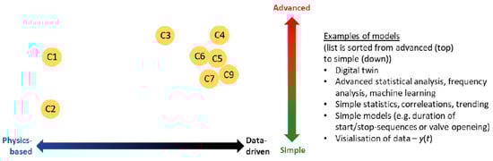
Figure 1.
Classification of anomaly detection problems.
In the study of Åsnes A. et al., methods for predictive state monitoring with real-time analysis methods based on continuous data flow in hydroelectric power plants are presented [3]. In this study, machine learning methods such as a support vector machine, neural networks and kernel density estimation were used for modeling. Hundi P. and Shahsavari R. [4] modeled the effect of various parameters on active power output by using supervised machine learning methods such as linear regression, multilayer sensors and support vector regression to facilitate the early detection of faults that may occur in combined cycle power plants. When the prediction outputs of the models created in the study were compared with the actual outputs, R2 scores were up to 96%, and the efficiency of these models against physics-based models was demonstrated. In the study by He K. et al. [5], it was stated that an excellent anomaly detection model is required to ensure the safe and economical operation of thermal power plants, and classical physics-based models are insufficient in this regard. An alternative model for anomaly detection is created as a more efficient solution by using the k-nearest neighbor algorithm, one of the machine learning methods, for primary air fans. Primary fans are one of the pieces of critical equipment in thermal power plants. In the study by Sambana B. et al., using physics-based modeling to detect problems related to bearing grease, which is one of the common bearing failures in wind farms, is challenging, while the measurements made with the support vector machine method are classified to make more precise and early bearing failure detection possible [6]. Performance and usability of methods such as adaptive neuro-fuzzy interface system (ANFIS), artificial neural networks, support vector machines, curve-fitting, etc., in hydroelectric power plants are presented in studies by Kumar K. and Saini R.P. [7,8]. In these comparative studies, efficiency and silt erosion are predicted with R2 scores of up to 0.999986. When methods to improve the operation and maintenance of hydropower plants are reviewed, it is seen that solutions employing SCADA, IoT and cloud-based monitoring systems, combined with condition-based monitoring methods such as fuzzy logic, AHP, PSO, ANN and SOM, play an important role [9]. The results in this paper are comparable with results from previous works on several power plants with R2 scores varying between 0.95–0.99 [4,7,8].
Malfunctions in hydraulic speed governors usually exhibit anomaly-indicating behaviors such as an increase in oil temperature, an increase in vibration and the noise level of motor–pump couples and a decrease in oil level. In classical control systems, these indicators are expected to be noticed/perceived by the system operators if they do not exceed the predefined thresholds. However, as the number of data increase, this requires the use of advanced analytical methods beyond visual and auditory evaluation. Considering the need for active threshold anomaly detection and the gap in the literature in this area, the study is of great importance. With the novel approach proposed in the research, which the literature lacks, the demanding task of detecting anomalies in hydraulic power units will be achieved in an easier, more successful way.
Figure 2 shows a real anomaly scenario that creates no alarm in conventional methodology. Due to nitrogen leakage in the hydraulic accumulators of the speed governor, the capacity of the accumulators dropped slowly and caused pumps to run more frequently, causing the oil to heat, pumps to wear faster and energy consumption to rise. In the figure, trends in governor oil pressure from the first month the system is commissioned (upper), 3rd month after commissioning (middle) and 8th month after commissioning (lower) are shown. It is easily seen that pumps ran 5–6 times per hour at the beginning; later, they reached 12–13 times per hour due to leakage. The methodology proposed in this study could detect this anomaly at the very beginning, probably less than a month after commissioning, before the problem worsens.
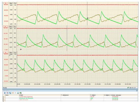
Figure 2.
An example of failure in a governor hydraulic unit without any warning.
2. Materials and Methods
As a result of the rapid digitalization of power plants, the use of modern control equipment in automation systems facilitates the collection of information from various electrical/mechanical systems and increases data diversity. Today, with the inclusion of modern SCADA systems with advanced storage/monitoring capabilities in these facilities, it is possible to record and analyze various data for the long-term with high resolution. In the control systems in modern HEPPs, various information is conveyed to the programmable logic controllers (PLC/Controller) that control the relevant subsystem through multiple sensors and switches distributed in the field. This information, which is in the form of raw signals, is digitized and converted into data by the controllers. While these data can be used in the controller’s own internal algorithms, they are also transferred to the servers so that the operators operating the system can view and record them over the human–machine interfaces. An example is depicted in Figure 3 showing a modern SCADA architecture in a hydropower plant.
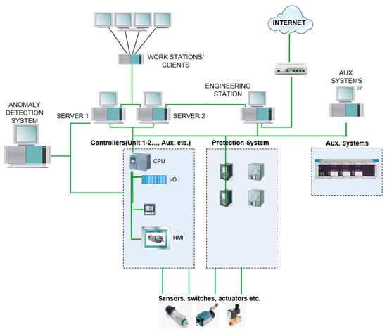
Figure 3.
SCADA architecture example.
2.1. Speed Governor
In hydroelectric power plants, the rotation turbine’s speed or active power output is controlled by the amount of water supplied to the turbine, depending on the operating mode. The amount of water flowing through the turbine is controlled by speed governors through adjustable gates located around the turbine called guide vanes. A general layout for a hydropower plant and the function of governors is given in Figure 4 [10].
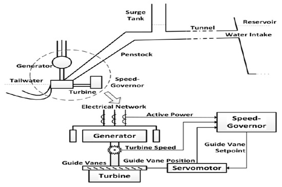
Figure 4.
General layout of a hydropower plant.
Speed governors consist of a hydraulic power unit and a control unit coupled to them containing control loops that ensure stable operation of the plant at the desired control point with the information collected from various sensors on this system. The guide vanes, which control the water at pressures that can vary from a few bars to tens of bars depending on the net head of the plant, are controlled by turning a circular mechanism called the regulation ring so that they can move together. Since the rotation of this ring requires great force, hydraulic pistons/servo motors and hydraulic power units are used with pressurized oil. The pressurized oil needed for the system in the examined power plant is supplied by two identical motor–pump sets controlled by the principle of co-aging and a hydraulic accumulator group filled by them. Since there is always a need for pressurized oil in the system, a hydraulic accumulator is used in order to prevent the pumps from running continuously and to supply pressurized oil in case the pumps are de-energized. The accumulator system consists of a nitrogen tank and a piston accumulator. It stores the pressurized oil needed by the system. When the system pressure drops below the preset level, one of the pumps runs, pressurizes the oil taken from the unpressurized oil tank and transmits it to the accumulators. This oil pushes the piston separating the oil, thus, ensuring the compression of the nitrogen. The pumps stop when the pressure reaches the preset upper limit and the pressurized oil is provided by the expansion of the compressed nitrogen.
Among the equipment in Figure 5, the parts at the back are the hydraulic accumulators, the parts at the front are the unpressurized oil tank and the various equipment, such as valves, transmitters, gauges, etc. The oil drawn from the unpressurized oil tank by the two motor–pump pairs on the tank is pressurized and stored in the accumulators. Then, it is used to control the guide vane opening via the analog controlled proportional valve, which is also seen in black on the tank.
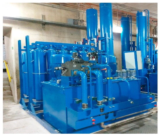
Figure 5.
Hydraulic power unit of the speed governor.
2.2. Modelling Methodology
The evaluation method to be used differs according to the diversity of the collected data and the complexity of the examined system. Welte and Foros [3] listed these methods from complex to simple as follows:
- (a)
- Digital twin
- (b)
- Advanced statistical analysis, frequency analysis, machine learning
- (c)
- Simple statistics, correlations, trends
- (d)
- Simple models (start/stop times, opening time of valves, etc.)
- (e)
- Visualization of data
Considering the complexity of the hydraulic unit and its changing characteristics under different operating conditions, machine-learning-based methods appear to be appropriate for the system in this study. Previously conducted similar studies for various mechanical systems show that, for anomaly detection, machine-learning-based models have numerous advantages over physical models.
Machine learning is briefly defined as the process of creating an inductive model that learns from a limited amount of data without expert intervention [11]. In traditional programming methods, the data are processed by the prepared program and converted into output. In contrast, in machine learning, the dataset and the event output are given to the computer and the program that associates them is expected to be created. This method was used for the first time in a checkers game designed by Arthur Samuel (IBM) in the 1950s, and the game’s self-development was ensured due to the dataset that expanded as the game played. The main difference between machine learning from conventional programming approaches is that the computer creates the model, as shown visually in Figure 6 [12].
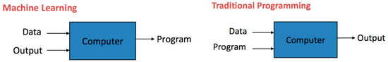
Figure 6.
Traditional programming versus machine learning.
2.2.1. Multivariable Linear Regression
Linear regression is a method in which the relationship of a dependent variable with an independent variable is modeled through a linear equation. Since it uses a single independent variable, this method cannot estimate the joint effect of other independent variables [13]. In this method, the relationship of the dependent variable with n independent variables was expressed by Singh et al. [14] as follows:
In the given expression, y is the dependent variable, β0, … βn are the coefficients, and x1, … xn are the independent variables. This method aims to find the β coefficients that will ensure that the error between the real y and the model output y, according to the several performance criteria mentioned in the following sections, is minimal.
2.2.2. Decision Tree Regression
Decision trees are one of the widely used machine learning methods in classification and regression problems. There are four essential elements in a decision tree [14];
Decision Node: The location where the tree will be split based on the argument and the value of the dataset.
Edge: Shows the direction of divergence when moving to the next node.
Root: The first node where the divergence starts.
Leaf node: It is the last node that predicts the outcome of the decision tree.
In this method, each feature in the dataset is considered a node. To evaluate the operation of the decision tree, we start from a node and continue down until our success criteria are met; this process continues until we reach the last node. The final node is the output of the decision tree, that is, the estimated value [14]. A schematic representation of this tree structure is given in Figure 7 [15].

Figure 7.
Decision tree schematic representation.
In the decision tree method, the data are divided in a way that minimizes entropy. Entropy was expressed mathematically by Claude Shannon (1948) as follows:
In this equation, p(x) denotes the percentage of the group belonging to a particular class, and H corresponds to entropy. The information gain used to minimize entropy is calculated as follows [16]:
In this equation, S is the original values of the dataset, and D is a part of it. Vs are discrete subsets of S. Information gain is the entropy difference of the data before and after the split [13].
2.2.3. Random Forest Regression
The random forest algorithm consists of a combination of decision trees. Each decision tree in this structure consists of a data sample obtained from the training set, and these are called bootstrap samples [17]. Estimation is performed as the mean of the independent decision trees.
In Figure 8, x represents the independent variables [18]. The estimated dependent variable y is obtained as a result of evaluating the independent variables in different decision trees and averaging them.
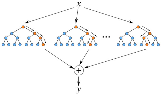
Figure 8.
Random forest schematic representation.
The methodology followed in the random forest algorithm can be summarized as follows [17]:
Step 1: Pairs of (Xi, Yi) are created. Here, X denotes the independent variables and Y represents the response variable.
Step 2: The bootstrap sample (X1*, Y1*), …, (Xn*, Yn*), which is obtained by randomly drawing n times by changing from the (X1, Y1), …, (Xn, Yn) data, is executed.
Step 3: Step 1 and Step 2 are repeated B times to obtain the following random forest convergence ().
2.2.4. Extreme Gradient Boosting (XGBoost) Regression
Gradient boosting is one of the widely used machine learning methods for regression and classification in various fields. The system prepared with the XGBoost method can run ten times faster than common methods on a single machine and can be scaled so that billions of samples can be processed in applications with limited memory [19].
An example diagram showing the operation of this structure is given in Figure 9 [20].
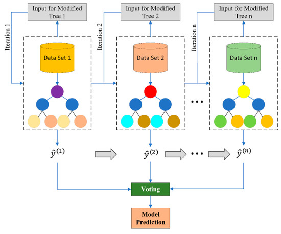
Figure 9.
XGBoost schematic representation.
In this method, ft’s are collected to minimize the following expression, with the i-numbered estimation component ŷi(t) in the t iteration [20].
2.2.5. Support Vector Regression
The support vector machine is a machine learning method that can be used for nonlinear regression and pattern recognition and is based on statistical learning theory and structural risk minimization theory. This method’s nonlinear regression application is called support vector regression [21]. The method was first proposed by Cortes and Vapnik and used by Vapnik in 1995 as a new type of universal learning machine that implements the strategy of keeping the empirical risk constant by minimizing the confidence interval [22].
The support vector regression aims to find the f(x) function that deviates from the target value yi by a maximum of ε as in Figure 10 for the entire training dataset [20]. For this purpose, if we define the line as:
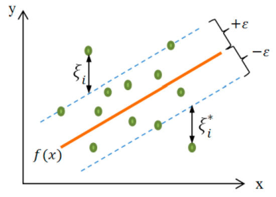
Figure 10.
Linear support vector regression.
What support vector regression should do is minimize the margin providing the condition [23]:
Which is calculated as:
2.2.6. Multilayer Perceptron
Multilayer perceptron or feedforward neural networks are the first artificial neural network structures designed and are widely used in modeling engineering problems [10]. It starts with the initial mesh weights set as a gradient; then the training algorithm tries to find the least error values by comparing the desired and actual outputs in a repeatable process until the network reaches acceptable values [24].
An example multilayer sensor structure is given in Figure 11 [25]. In the figure, the number of the hidden layer(s) is only 1, but it varies according to the complexity of the problem.
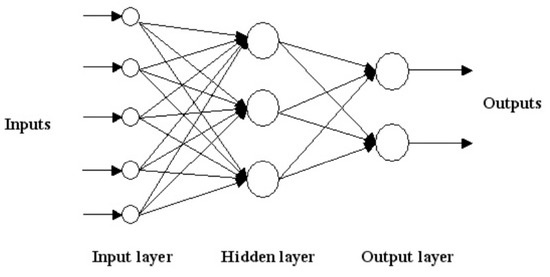
Figure 11.
Multilayer Perceptron Schematic Representation.
The schematic representation of the nonlinear neurons in this structure is given in Figure 12 [26]. In this model, each of the inputs (x1, x2, …) is weighted with parameters called synaptic weight (k1, k2…) and collected in the aggregation link. This total is sent to an activation function (φ(.)) that limits the output of the neuron to a finite value, and the output of the relevant neuron is formed. The bias (bk) added to the sum before the activation function is used to increase or decrease the effect of the relevant neuron, depending on whether it is positive or negative [26]. Based on feedforward backpropagation, this model aims to achieve the best result by updating the synaptic weights by feeding back the error in each forward iteration. Mathematically, the relationship between these parameters can be expressed as follows:
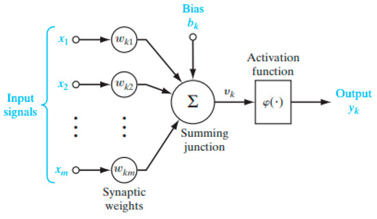
Figure 12.
Nonlinear Neuron Model.
2.3. Modeling Environment
Python is an interpreted programming language, first introduced in 1991, designed to emphasize code readability, and draws inspiration from several programming algorithms such as procedural languages (similar to C), object-oriented languages (similar to Java) and functional languages (similar to Lisp, Haskell) [27]. This programming language is one of the most popular programming languages for data science. Since it is open source with its developer, many useful libraries for scientific computing and machine learning were developed [28]. While creating the models in the study, the 3.9 version of the Python programming language and various libraries prepared with this language were used. The Eclipse (Eclipse Jee 2019-6) program was preferred as the development environment.
Scikit Learn is a rich library integrated with the python language, easy to use and contains state of the art applications of many machine learning algorithms. The software responds to the growing need for statistical data analysis by the web industries and non-computer science specialists such as biology and physics [29]. This library forms the basis of most of the machine learning algorithms used in the study. Within the scope of this study, we used the LinearRegression function from sklearn.linear_model library, DecisionTreeRegressor function from sklearn.tree library and the RandomForestRegressor.svm function from sklearn.ensemble library for multivariate linear regression, decision tree, random forest and support vector regressions, respectively. SVR in the library and MLPRegressor functions in the sklearn.neural_network library were used. By changing the parameters of these functions, an attempt at optimization was made to obtain the most successful estimation. For extreme gradient boosting, the XGBRegressor function in the open source xgboost library was used.
In order to increase the accuracy of the models, before using the train or test data as input to functions, the data were normalized to be mean(µ) 0 and variance(σ) 1 using the Preprocessing.StandardScaler function imported from the Scikit-Learn(sklearn) library. While comparing the estimated dependent variable with the actual measurements and obtaining the performance parameters, mean_squared_error, r2_score and mean_absolute_error commands in the sklearn.metrics library were used. Furthermore, in an externally created while loop, the predicted points with less than ±1% and ±5% errors were counted and divided by the number of points in the dataset. The outputs obtained from these were added to the performance criteria and presented among the results. Mathematical representations of mean absolute error (MAE), root mean squared error (RMSE) and mean square error (MSE) are as follows [8]:
where is the output of the model (prediction), is the value measured from the system and N is the number of samples. R2 score is obtained by squaring the correlation parameter R, which is calculated as:
2.4. Datasets
Hydraulic speed governor oil pressure depends on many parameters. For example, since the oil sent to the accumulator is drawn from the unpressurized oil tank, it is expected that the oil level in the tank will decrease while the accumulator pressure rises. It can be expected that the pressure oil consumption in the system will be the least when the system is stationary, and the oil consumption will be the highest during start and stop sequences that cause the pistons to move the most. Various parameters that can be associated with pressure in similar ways and their correlation with each other are shown in Figure 13. This figure was obtained from the training dataset used in the study, and the seaborn.heatmap function in seaborn, one of the Python libraries, was used to visualize it.
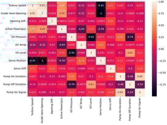
Figure 13.
Heatmap showing the correlation between parameters in the training dataset.
After eliminating data having no or negative effect on model performance, it was deemed appropriate to use the ones listed below with a resolution of 1 s. While selecting these data, the correlation values with the dependent variable, field experiences and model performance data obtained from various trials/tests were used.
Independent variables:
- (a)
- Servo difference: The change in the position of one of the servomotors according to the measurement of previous second
- (b)
- Active Power (pu): The normalized active power of the generator
- (c)
- Oil Temperature: The temperature of the oil in the unpressurized oil tank
- (d)
- Oil Level: The percentage value of the oil amount in the unpressurized oil tank
- (e)
- Pump On Time: The length of time that one of the identical pumps works each time it is activated
- (f)
- Pump Off Time: The length of time from stopping the pump to restarting
Dependent variables:
- (g)
- Oil Pressure: The pressure of the oil used in the system, hence, in the accumulator
In the study, data are obtained from a hydraulic governor of a large hydropower unit. From speed, temperature, pressure, position sensors and soft starters of oil pumps, measurements and on-off information were collected by Siemens S7-1500 series programmable logic controllers and recorded on SCADA servers in a hierarchy similar to the one given in Figure 3. Some of the measuring devices and their places can be seen in Figure 14.
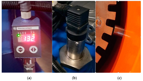
Figure 14.
Some of the measuring points, oil pressure (a), oil level (b), turbine speed (c).
The data to be used as a training dataset, which includes different working conditions recorded at different times with a one-second sampling period, are shown in the graph given in Figure 15. While creating this data group, data from various operating conditions were included in the group so that the model could show high performance in different operating conditions. Since the amount of movement(mm) per second and applied forces on the guide vanes change in different operating conditions, a comprehensive data group was formed by taking data from the start sequence, stop sequence, long-term stop and long-term loaded running conditions of the unit. As a result, a set consisting of 10,529 points was obtained. The main focus while creating the dataset was not the number of points but the inclusivity of different conditions. For example, in order to include the effect of oil temperature, data at different times in the range of 20–34 degrees were included in the training group. As seen in the graph, the behavior of the pressure during the rise and fall may vary according to the operating conditions. It can be easily understood from the slope changes and breaks in the pressure curve that the pressure drops faster than normal as a result of opening the guide vanes through servomotors during the commissioning of the unit and moving it over the stationary state until it reaches the speed–power set point.
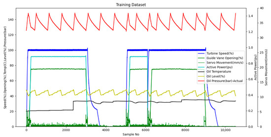
Figure 15.
Training dataset without pump status.
In Figure 16, the operating time of any of the identical two pumps that provide the system pressure and the time from reaching the target pressure and stopping until it starts again are shown. These parameters are also included as independent variables in the training data group. In the exemplified operating conditions, it was observed that the time for the pump to reach the maximum pressure of the accumulator varies between 80–116 s, and the pressure discharge time varies between 300–642 s. These change amounts reveal the inadequacy of creating alarms using the classical approach, which is the predefined threshold value.

Figure 16.
Training dataset pump on/off durations.
For validation of the models before testing with data from different times, the training dataset is randomly divided into parts of 70% and 30%. The model is trained with 70% and validated with 30% several times to make sure the model runs stably. Then, the created model is tested with a dataset from different time intervals not intersecting with the training group to ensure that the model is reliable to use in online anomaly detection with live data from real equipment.
While creating the test data group, in order to reveal the performance of the model in real working conditions in the most accurate way, instead of randomly separating the data as a training-test data group from a dataset that follows each other in time, the data in the training data group were preferred from the working conditions at a different time than they belonged to. The data group used for testing is shown in Figure 17. The main focus while creating the dataset is not the number of points but the inclusivity of different conditions. In order to test the model performance in different operating conditions, an inclusive dataset is created with a sampling time of one second. As a result, a test group consisting of 14,341 points is obtained. This test group includes data from different operating conditions such as steady state, rated load operation, starting and stopping.
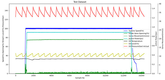
Figure 17.
Test dataset without pump status.
Figure 18 shows the time between the operation of the oil pumps in the test group and the time between the operation and re-start after stopping. As can be seen from the graph, the longest time without a pump occurred when the unit was stationary. When starting the unit, the minimum pressure was reached and one of the pumps was activated during the time when the oil consumption was high. During this period, the longest pump operating time of this data group occurred as the accumulator was filled while the high consumption continued. In this graph, the operating time of the pumps at a single start-up was in the range of 81–107 s, while the time for the accumulators to discharge and reach the pump operating pressure without the pump running was in the range of 388–623 s.
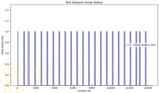
Figure 18.
Test dataset pump on/off durations.
3. Results
In this study, a hydropower plant’s hydraulic governor was modeled using a training dataset with various methods, and the prediction was made on the test data, and the results seen in Table 1 were obtained. As can be seen in the table, the most successful model was obtained with random forest regression according to the ability to predict with less than 1% absolute error, while support vector regression revealed the most unsuccessful results in this study. The fact that the random forest method evaluates the outputs of many decision trees together resulted in an 8% higher success rate of the decision tree method, and estimated 96.45% of the outputs with less than 1% absolute error and less than 100% of them with 5% absolute error. It was observed that the linear regression method is insufficient in modeling the nonlinear behavior of parameters such as temperature and pressure due to the delay time in response to changes, and this is demonstrated by the low performance parameters.

Table 1.
Pressure prediction test performance results.
The estimation outputs of the random forest regression method, which gives the closest estimation results according to the success criteria, are given in Figure 19 in comparison with the actual values. When the estimated and actual oil pressure values are compared on the graph, the visual consistency of the high mathematical success rates can be observed. The model is able to predict the discharge curves of the accumulator with high accuracy, as seen in Table 1 and Figure 19, with the filling–discharging cycles in the test data group, which includes the cases where the accumulators are filled and discharged 23 times, with the accumulator filling completed in the range of 81–107 s and the oil discharge time varying between 388–623 s.
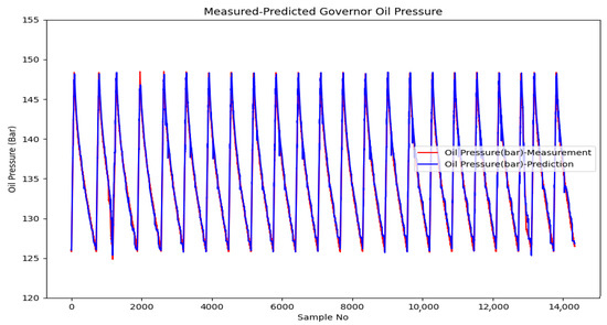
Figure 19.
Predicted-measured governor system pressure.
The prediction results in the interval where the unit operates at the rated load are shown in Figure 20. As can be seen in this graph, the estimated and actual pressure values are consistent, except for the deviations occurring at a few points.
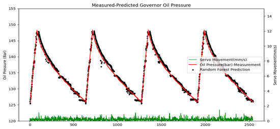
Figure 20.
Predicted–measured governor system pressure under constant load.
4. Discussion
The fill-and-discharge curve of the accumulators in the hydraulic power unit of the speed regulator of the hydroelectric unit was modeled under different oil consumption conditions. As a result of the study, it was observed that the instantaneous pressure level could be predicted with R2 scores up to 0.985 and an absolute error of less than 1% up to 96.45%. Absolute error rates were found by counting the absolute deviations from the true value by less than a percentage specified and dividing by the total number of data. R2 scores, widely used as an indicator of regression in the field of statistics, where the most successful ratio is accepted as 1, were calculated using the “sklearn.metrics” library of python. When the error rate in pressure inspection is increased to 5%, all of the methods can predict with an accuracy of 99–100%. The most successful result was obtained with random tree regression, and the most unsuccessful result was obtained with support vector regression. Decision trees are flexible to model higher order non-linearity and insensitive to outliers in the covariate space [30]; tree based models, which are decision tree, random forest and xgboost regression, resulted in comparably better results than other methods. In the light of the results of this study, it can be concluded that the pressure estimation data can be used to detect anomalies in the system by considering the 1% margin of error, which is way better than the conventional approach, which usually considers thresholds over 10%.
5. Conclusions
In this study, machine-learning-based anomaly detection approaches in hydroelectric power plants were introduced; for this purpose, six different algorithms were implemented and tested with data from an operational system, and we planned to create more comprehensive models by including different systems and different sensors, such as vibration and acoustic sensors, in the future studies. For further research, the number of methods for modeling can be increased, and selection can be automatized to pick the proper method from a more extensive set of options for different systems, which is one of the difficulties of the work. In the following periods, using this innovative method, the status of the systems will be monitored live and the failures will be detected in advance with the decision support software to be created. By evaluating the deviations between the model output and the measurements performed, predictive maintenance studies can be carried out on the equipment. The remaining useful lives can be predicted by evaluating the wear rates. With the dissemination of the solution, hydropower plants will be able to be operated with fewer people, and negative situations caused by human error will be minimized. With the efficient use of energy, the adverse environmental effects caused by electrical energy production can be reduced by these methods. Due to the early detection of the factors that have a negative impact on efficiency, more electrical energy will be produced by using fewer resources.
Author Contributions
Conceptualization, M.A.B., İ.K. and D.G.; data curation, M.A.B.; formal analysis, M.A.B., İ.K. and D.G.; investigation, M.A.B.; methodology, M.A.B., İ.K. and D.G.; project administration, D.G.; resources, M.A.B. and D.G.; software, M.A.B.; supervision, İ.K.; validation, M.A.B.; visualization, D.G.; writing—original draft, M.A.B. and İ.K.; writing—review and editing, M.A.B., İ.K. and D.G. All authors have read and agreed to the published version of the manuscript.
Funding
This research received no external funding.
Data Availability Statement
The data presented in this study are available on request from the corresponding author.
Acknowledgments
The authors gratefully acknowledge the contributions of TUBITAK MRC through supporting this research study by the project numbered 5172804 and conducted at TUBITAK, Scientific and Technological Research Council of Turkey, Marmara Research Center (MRC) Energy Technologies Vice Presidency.
Conflicts of Interest
The authors declare no conflict of interest.
References
- International Renewable Energy Agency. Renewable Capacity Highlights; International Renewable Energy Agency: Abu Dhabi, United Arab Emirates, 2021. [Google Scholar]
- Welte, T.; Foros, J. Monitor X—Digitalization in Hydropower. 2019. Available online: https://energiforsk.se/media/26984/monitor-x-energiforskrapport-2019-618.pdf (accessed on 8 June 2022).
- Åsnes, A.; Willersrud, A.; Imsland, L. Predictive maintenance and life cycle estimation for hydro power plants with real-time analytics. In Proceedings of the Hydro 2018, Gdansk, Poland, 15–17 October 2018. [Google Scholar]
- Hundi, P.; Shahsavari, R. Comparative studies among machine learning models for performance estimation and health monitoring of thermal power plants. Appl. Energy 2020, 265, 114775. [Google Scholar] [CrossRef]
- He, K.; Wang, T.; Zhang, F.; Jin, X. Anomaly detection and early warning via a novel multiblock-based method with applications to thermal power plants. J. Int. Meas. Confed. 2022, 193, 110979. [Google Scholar] [CrossRef]
- Sambana, B.; Appala Naidu, P.; Jarabala, R.; Narayana, V.N.S.L. Performance validation of wind turbines using machine learning methodologies. Mater. Today Proc. 2022. [Google Scholar] [CrossRef]
- Kumar, K.; Saini, R.P. Adaptive neuro-fuzzy interface system based performance monitoring technique for hydropower plants. ISH J. Hydraul. Eng. 2022, 1–11. [Google Scholar] [CrossRef]
- Kumar, K.; Saini, R.P. Development of correlation to predict the efficiency of a hydro machine under different operating conditions. Sustain. Energy Technol. Assess. 2022, 50, 101859. [Google Scholar] [CrossRef]
- Kumar, K.; Saini, R.P. A review on operation and maintenance of hydropower plants. Sustain. Energy Technol. Assess. 2022, 49, 101704. [Google Scholar] [CrossRef]
- Gezer, D.; Taşcıoğlu, Y.; Çelebioğlu, K. Frequency containment control of hydropower plants using different adaptive methods. Energies 2021, 14, 2082. [Google Scholar] [CrossRef]
- Cui, B.; Weng, Y.; Zhang, N. A feature extraction and machine learning framework for bearing fault diagnosis. Renew. Energy 2022, 191, 987–997. [Google Scholar] [CrossRef]
- Brownlee, J. Basic Concepts in Machine Learning. Available online: https://machinelearningmastery.com/basic-concepts-in-machine-learning/ (accessed on 20 July 2022).
- Demirbay, B.; Bayram Kara, D.; Uğur, Ş. Multivariate regression (MVR) and different artificial neural network (ANN) models developed for optical transparency of conductive polymer nanocomposite films. Expert Syst. Appl. 2022, 207, 117937. [Google Scholar] [CrossRef]
- Kushwah, J.S.; Kumar, A.; Patel, S.; Soni, R.; Gawande, A.; Gupta, S. Comparative study of regressor and classifier with decision tree using modern tools. Mater. Today Proc. 2022, 56, 3571–3576. [Google Scholar] [CrossRef]
- Chauhan, N.S. Decision Tree Algorithm, Explained. Available online: https://www.kdnuggets.com/2020/01/decision-tree-algorithm-explained.html (accessed on 24 August 2022).
- Ülgen, K. Makine Öğrenimi Bölüm-5 (Karar Ağaçları). Available online: https://medium.com/@k.ulgen90/makine-öğrenimi-bölüm-5-karar-ağaçları-c90bd7593010 (accessed on 24 August 2022).
- Kaygusuz, M.A.; Purutçuoğlu, V. Random forest regression and an alternative model selection procedure. In Proceedings of the 2nd International Conference on Applied Mathematics in Engineering, Balikesir, Turkey, 1–3 September 2021. [Google Scholar]
- Bakshi, C. Random Forest Regression. Available online: https://levelup.gitconnected.com/random-forest-regression-209c0f354c84 (accessed on 24 August 2022).
- Chen, T.; Guestrin, C. XGBoost: A scalable tree boosting system. In Proceedings of the International Conference on Knowledge Discovery and Data Mining, 13–17 August 2016; pp. 785–794. [Google Scholar]
- Shehadeh, A.; Alshboul, O.; Al Mamlook, R.E.; Hamedat, O. Machine learning models for predicting the residual value of heavy construction equipment: An evaluation of modified decision tree, LightGBM, and XGBoost regression. Autom. Constr. 2021, 129, 103827. [Google Scholar] [CrossRef]
- Li, S.; Xu, K.; Xue, G.; Liu, J.; Xu, Z. Prediction of coal spontaneous combustion temperature based on improved grey wolf optimizer algorithm and support vector regression. Fuel 2022, 324, 124670. [Google Scholar] [CrossRef]
- Alcaraz, J.; Labbé, M.; Landete, M. Support Vector Machine with feature selection: A multiobjective approach. Expert Syst. Appl. 2022, 204, 117485. [Google Scholar] [CrossRef]
- Chanklan, R.; Kaoungku, N.; Suksut, K.; Kerdprasop, K.; Kerdprasop, N. Runoff prediction with a combined artificial neural network and support vector regression. Int. J. Mach. Learn. Comput. 2018, 8, 39–43. [Google Scholar] [CrossRef]
- Razavi, B.S. Predicting the Trend of Land Use Changes Using Artificial Neural Network and Markov Chain Model (Case Study: Kermanshah City). Res. J. Environ. Earth Sci. 2014, 6, 215–226. [Google Scholar] [CrossRef]
- Sazli, M.H. A Brief Review of Feed-Forward Neural Networks. Commun. Fac. Sci. Univ. Ank. Ser. 2006, 50, 11–17. [Google Scholar] [CrossRef]
- Haykin, S. Neural Networks and Learning Machines, 3rd ed.; Dworkin, A., Ed.; Pearson Education: North York, ON, Canada, 2009; Volume 1–3, ISBN 9780128114322. [Google Scholar]
- Thomas, J. Why Python? 2012. Available online: https://www.math.arizona.edu/~swig/documentation/python/handout.pdf (accessed on 27 July 2022).
- Raschka, S.; Mirjalili, V. Python machine learning: Machine learning and deep learning with python, scikit-learn, and tensorflow. Int. J. Knowl. Based Organ. 2021, 11, 741. [Google Scholar]
- Pedregosa, F.; Grisel, O.; Weiss, R.; Passos, A.; Brucher, M.; Varoquax, G.; Gramfort, A.; Michel, V.; Thirion, B.; Grisel, O.; et al. Scikit-learn: Machine Learning in Python. J. Mach. Learn. Res. 2011, 12, 2825–2830. [Google Scholar]
- Taherdangkoo, R.; Liu, Q.; Xing, Y.; Yang, H.; Cao, V.; Sauter, M.; Butscher, C. Predicting methane solubility in water and seawater by machine learning algorithms: Application to methane transport modeling. J. Contam. Hydrol. 2021, 242, 103844. [Google Scholar] [CrossRef] [PubMed]


Publisher’s Note: MDPI stays neutral with regard to jurisdictional claims in published maps and institutional affiliations. |
© 2022 by the authors. Licensee MDPI, Basel, Switzerland. This article is an open access article distributed under the terms and conditions of the Creative Commons Attribution (CC BY) license (https://creativecommons.org/licenses/by/4.0/).