Regionalization of Climate Change Simulations for the Assessment of Impacts on Precipitation, Flow Rate and Electricity Generation in the Xingu River Basin in the Brazilian Amazon

Abstract

This study applied regionalization techniques on future climate change scenarios for the precipitation over the Xingu River Basin (XRB) considering the 2021–2080 horizon, in order to assess impacts on the monthly flow rates and possible consequences for electricity generation at the Belo Monte Hydroelectric Power Plant (BMHPP). This is the fourth largest hydroelectric power plant in the world, with a generating capacity of 11,233 MW, and is located in the Brazilian Amazon. Two representative concentration pathways (RCP 4.5 and RCP 8.5) and an ensemble comprising four general circulation models (CanESM2, CNRM-CM5, MPI-ESM-LR and NORESM1-M) were used. The projections based on both scenarios indicated a considerable decrease in precipitation during the rainy season and a slight increase during the dry season relative to the reference period (1981–2010). According to the results, a reduction in the flow rates in Altamira and in the overall potential for power generation in the BMHPP are also to be expected in both analyzed periods (2021–2050 and 2051–2180). The RCP 4.5 scenario resulted in milder decreases in those variables than the RCP 8.5. Conforming to our findings, a reduction of 21.3% in the annual power generation at the BMHPP is expected until 2080, with a corresponding use of 38.8% of the maximum potential of the facility. These results highlight the need for investments in other renewable energy sources (e.g., wind and solar) in order to compensate for the upcoming losses in the BMHPP production.

1. Introduction

In the context of electricity production, Brazil is among the countries in possession of the greenest portfolios, with its total primary energy supply being presently comprised of the following contributions: 64.1% from hydropower, 22.9% from thermal sources, 9% from wind and 4% from other sources, such as nuclear, solar and others [1]. Since climatic variations influence the volume of water available in the reservoirs for hydroelectricity generation, the establishment of rules for the operation of hydropower plants must take into consideration the availability of water resources based on reliable future scenarios [2].

The Xingu River Basin (XRB) is located in Brazil’s Legal Amazon (as defined in IBGE, 2022—https://www.ibge.gov.br/en/geosciences/environmental-information/vegetation/17927-legal-amazon.html?edicao=30976&t=o-que-e (accessed on 10 July 2022) and hosts one of the largest projects of the Brazilian government in terms of electricity generation, Belo Monte Hydroelectric Power Plant (BMHPP), which is the fourth largest hydroelectric power plant in the world by installed capacity, representing the greatest energy enterprise that is entirely Brazilian. Since the completion of its construction in 2019, the installed capacity was 11,233 MW, which is equivalent to almost 10% of the Brazilian electricity demand [3,4].

Studies on the operational planning, management of and investments in power generation from hydroelectric plants in Brazil, especially in the Amazon Basin, have been carried out frequently [5,6]. Climate projections based on future scenarios indicate negative trends in rainfall over the Amazon [7,8], which underline the sensitivity of the region’s hydroelectric systems to climate variability, as the river flow rates are naturally correlated with the precipitation over their respective basins, with significant impacts on hydropower generation being expected.

There are considerable uncertainties, however, in the simulations from Global Climate Models (GCM) in relation to precipitation patterns and climate change [9]. Due to the coarse resolution of the GCMs, it is necessary to apply downscaling techniques, which converts information from large to regional or local scales [10]. The models are also forced through the implementation of boundary conditions, which are determined by the emission scenarios. This ends up consisting of another source of uncertainty in the projections [11]. The combination of different sources of uncertainty can lead to unrealistic projections of precipitation and of the impacts of climate change on hydrology [12,13]. Some options have been applied in order to reduce the uncertainties in the projections of the impacts of climate change, such as the use of sets of several models (ensembles) and statistical post-processing on the data, aimed at removing biases [13,14].

Through the use of the Coupled Model Intercomparison Project (CMIP5), some works have pointed to possible scenarios of climate change in South America and in Brazil, specifically, until the end of this century [15,16]. For the Amazon, in general, the projections indicate a decrease in precipitation and, consequently, in flow rates [7,17,18], as well as an increase in temperature [19]. Studies have been reporting that numerical models fail to capture important aspects of climate variability in the Amazon [8,20]. According to them, a poor representation of the atmospheric systems that cause precipitation over the Amazon and the difficulty in adequately representing the variability of the sea surface temperature anomalies on the tropical Pacific and Atlantic Oceans may be responsible for the underestimation of precipitation in the region.

In light of the above, the main purpose of this work is to obtain future regionalized scenarios of climate change for precipitation over the XRB, considering the 2021–2080 horizon and then assess their impacts on the monthly flow rates and the possible consequences for the power generation in the BMHPP. The results may aid in the improvement of planning and operation of the Belo Monte reservoir with regards to hydropower production. In addition to the known electricity potential, the XRB is of extreme relevance as an environmental and cultural asset, as it encompasses not only part of the Amazon rainforest, but also extensive portions of the Cerrado biome (the Brazilian savannah), as well as protected forest areas and indigenous territories.

2. Materials and Methods

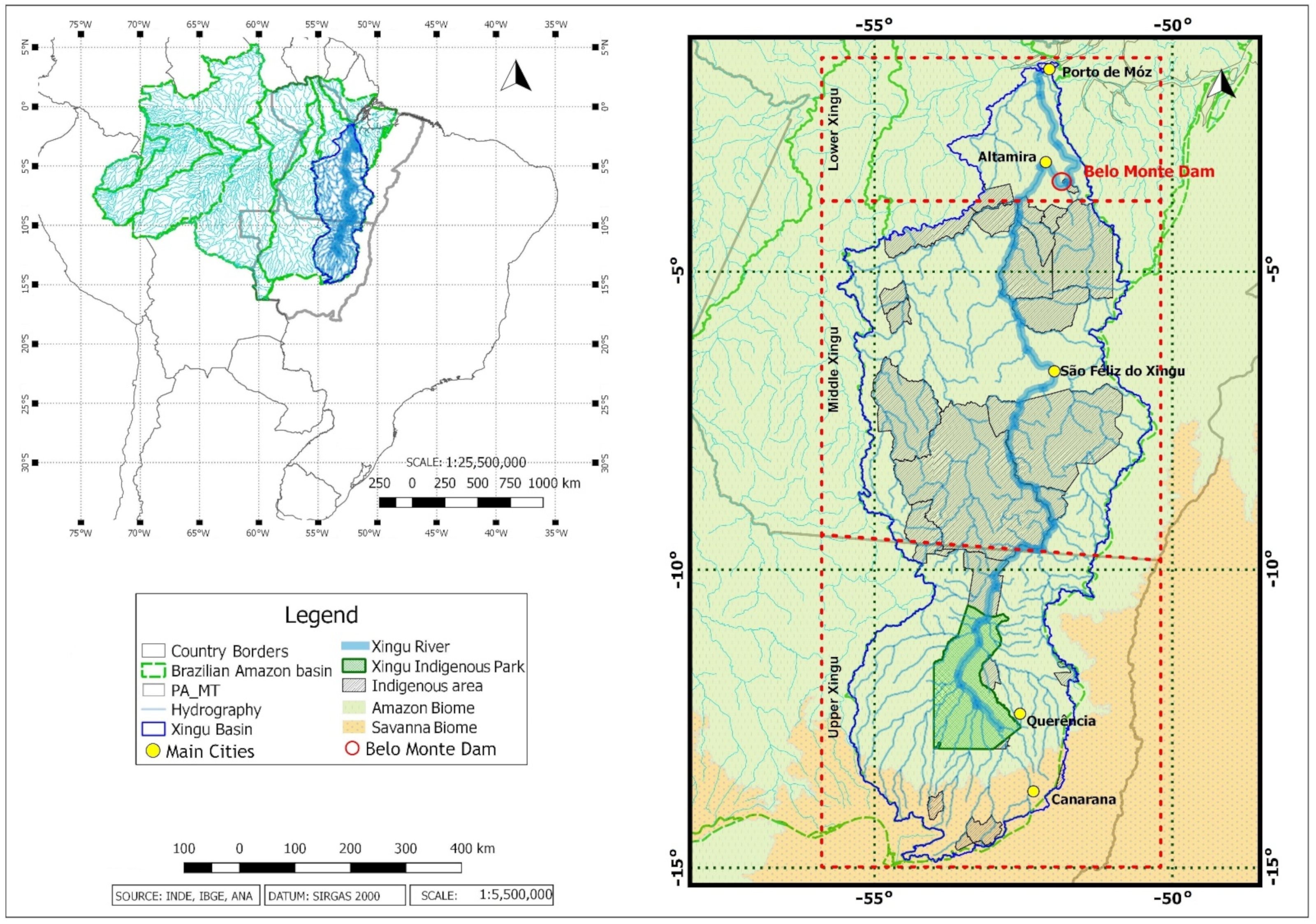
2.1. Region of Study

The XRB encompasses about 13% of the Amazon River Basin area that is located in Brazil, spanning across the states of Pará and Mato Grosso (Figure 1), with a total drainage area of around 510,000 km². The main river, Xingu, has its source in Mato Grosso, at an altitude of 600 m, at the meeting of Formosa and Roncador ridges, in the Brazilian Cerrado, and then joins the Amazon biome covering an extension of approximately 2000 km up to its mouth in the Amazon River, at an altitude of 4 m [21]. The XRB exhibits a south–north orientation and is basically divided into three regions: Upper Xingu, Middle Xingu and Lower Xingu. The main tributaries are the Iriri, Fresco, Curuá, Culuene and Bacajá rivers [22].

The XRB hosts two important Brazilian biomes (Amazon Forest and Cerrado) and about 280,000 km² of protected areas and indigenous territories, such as the Xingu Indigenous Park, one of the largest forest conservation areas in Brazil, comprising nearly 26,000 km². In spite of representing only 5% of the XRB area, the park is home to several ethnic groups, in addition to an exuberant fauna and flora. That territory is constantly threatened by anthropic actions, such as deforestation aimed at expanding agriculture and livestock frontiers. This has been taking place across the entire area surrounding the park [23,24].

The spatiotemporal variability of precipitation over the XRB exhibits different regimes between the northern and southern portions of the basin. In the south, as well as in the center, the largest rainfall volumes are observed in the months of December, January and February (DJF), owing to the South Atlantic Convergence Zone. Conversely, in the north, precipitation is concentrated in the period from February to April, when the northern part of the basin is within the reach of the Intertropical Convergence Zone, the atmospheric system that governs the rainfall regime of most of the Amazon [25,26,27].

The characteristic flow rate parameters of the XRB (long-term average flow rate and Q95—flow permanence of 95%) were calculated by the Brazilian National Water and Sanitation Agency (ANA) from monthly mean flow rates recorded by their network of river gauge stations [28]. Their study shows that the XRB has a long-term average flow rate of 8548 m³/s and a Q95 of 1184 m³/s. Water availability is the amount of water effectively available for different uses in the basin. Thus, identifying the availability of flow rate intended for meeting important demands is an essential part of a water resources plan.

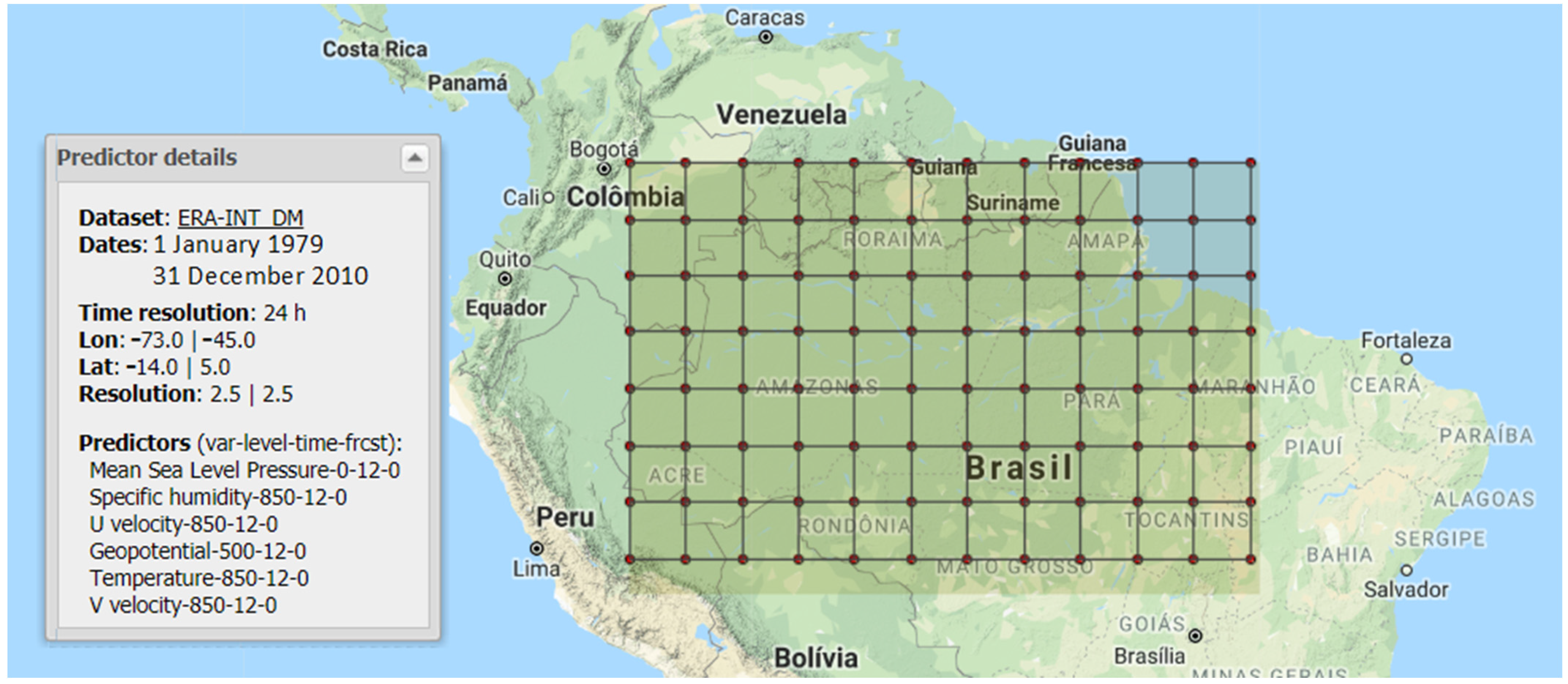
2.2. Future Emission Scenarios and GCMs

This work investigated the influence of climate change caused by the continuous increment in greenhouse gases concentration from scenarios of radiative forcing projected by the Intergovernmental Panel on Climate Change [29]. The RCP 4.5 and RCP 8.5 scenarios were used for the generation of predicted precipitation series over the XRB in the period 2021–2080. The results are presented and discussed for two different three-decade periods, 2021–2050 and 2051–2080, thus comprising two climatological normals. The characteristics of the two employed Representative Concentration Pathways are described in Refs. [30,31,32].

The GCMs from CMIP5 used here were: “CanESM2”, which stands for the second generation Canadian Earth System Model [33,34]; “CNRM-CM5”, which is the GCM of the (French) National Centre for Meteorological Research (CNRRM) and Centre Européen de Recherche et de Formation Avancée en Calcul Scientifique (CERFACS) [35,36]; “MPI-ESM-MR”, which is the Earth System Model (ESM) developed by the Max Planck Institute for Meteorology, based in Germany [37,38]; and NORESM1-M”, the Norwegian ESM of the Norwegian Climate Center [39,40].

Precipitation data were generated through the Data Access and Downscaling (DAD) Portal developed by the Santander Meteorology Group (https://www.meteo.unican.es/downscaling/intro.html, accessed on 10 January 2022). The applied Statistical Downscaling Method (SDM) used daily data of large-scale variables from the ERA-INT-DM reanalysis project from the period 1979–2010, with a spatial resolution of 2.5° × 2.5° and observed daily precipitation data from gauge stations located in Amazon that are operated by the (Brazilian) National Institute of Meteorology, from the same period.

SDMs consist of finding an empirical relation (a statistical model) between large-scale variables from reanalysis (predictors) and variables observed at smaller scales (predictands). Then, the resulting statistical model is applied to the data from different climate change simulations by GCMs and different scenarios [41,42]. A detailed review of statistical downscaling methods is presented in Ref. [43].

Figure 2 presents the resolution grid over the Amazon region that was applied to the SDM for the generation of the precipitation data used in this study, focusing on the XRB area. Further information related to the reanalysis data used as predictors in the SDM is also exhibited in Figure 2, such as the spatial and temporal resolutions, the identification of the variables, and the respective atmospheric levels and time of the day for which their values were obtained. The variables include: Mean Sea Level Pressure, Temperature and Specific Humidity at 850 hPa, Geopotential Height at 500 hPa and Meridional and Zonal Velocities at 850 hPa. A detailed description of this reanalysis can be found in Ref. [44], which describes the prediction model, the data assimilation method and the employed input dataset from observational data, in addition to discussing improvements in relation to previous reanalysis data, ERA-40.

Calibration and validation of the statistical downscaling was performed by employing the Analogue Method, which is thoroughly described in Refs. [45,46,47]. The common historical period for predictors (reanalysis) and predictands (observations) was divided into two different periods: 1979–2010 for training and 2011–2020 for comparison of results. The calibration used data from the training period to verify the climate similarity between observations and simulations, i.e., if the past climate was well represented by the predictors, relative to the period 1979–2010. The descriptive statistical metrics are described in Section 2.5, based on data accumulated in monthly values, which were used in the model for simulating monthly flow rates at the XRB.

Some works have been employing SDMs for obtaining local information from integrations by GCMs [48,49]. Ref. [50] applied the Analogue Method as a simple technique of statistical downscaling for scale reduction of a GCM for monthly and daily precipitation over the Iberian Peninsula during winter and performed a comparison with more complex methods, such as canonical correlations and neural networks. In general, the Analogue Method rendered satisfactory results relative to the other methods and could be applied to local variables with normal distributions or not. Those authors concluded that the neural networks, despite being more complex, do not provide a direct physical relation.

Based on the observed underestimation of the precipitation simulations for the training period (see Section 3.1), we resorted to the Linear Scaling method to estimate a correction factor for the monthly precipitation data generated by the SDM. Then, we performed bias removal, based on that correction factor, on the future precipitation series for the simulations of data for each station. This methodology of bias correction results in considerable benefits to research, as described by Ref. [16]. According to Ref. [51], GCM results are biased in the simulations of precipitation, which leads to flow-rate simulations that are also biased. However, the methods of bias correction can improve the simulated precipitation and the representation of flow rates in river basins.

Linear Scaling is a simple method to correct variables based on the observed long-term average [52]. Precipitation is corrected by multiplying the simulated value by a factor that is based on the ratio between the long-term averages of the observed and simulated data, as in the following equation:

$$P_{sim}^{cor} \left(t\right)=P_{sim} \left(t\right)\times \left[\frac{u {(}_{obs}^{hist }\left(t\right))}{u{(}_{sim}^{hist }\left(t\right))}\right]$$

(1)

where $P_{sim}^{cor} \left(t\right)$ is the corrected simulated precipitation for time t, $P_{sim} \left(t\right)$ is the simulated precipitation for time t, $u {(}_{obs}^{hist }\left(t\right))$ is the long-term average of the observed precipitation over the historical period and $u{(}_{sim}^{hist }\left(t\right))$ is the long-term average of the simulated precipitation over the historical period.

2.3. Rainfall–Runoff Model

The application of the hydrological modeling of rainfall–runoff through statistical techniques (empirical models) has been a growing tendency for the past few decades, especially because of the lack of some input data to conceptual models, the need for faster, reliable and less complex predictions. Therefore, we resorted to the Principal Component Regression (PCR) technique for the rainfall–runoff modeling for the XRB, in order to simulate monthly flow rates. The river gauge station of Altamira will be used as the reference for the validation of the simulation results of flow rates and the assessment of future scenarios. The river basins in the Amazon are particularly suitable for the application of hydrological rainfall–runoff models, as the precipitation and flow rates are highly correlated in these basins.

The regression by principal components was initially proposed by Refs. [53,54]. Such regression technique is based on Principal Component Analysis, with the purpose of overcoming difficulties found in Multiple Linear Regression, by eliminating problems of multicollinearity between the variables, as well as decreasing the level of noise that is entered into the model. Mathematical details about the application of this technique of multivariate statistical analysis are described in Refs. [55,56].

Ref. [57] applied the PCR technique in the simulation of monthly mean flow rates at the XRB. That study showed the degree of the relationship between precipitation and flow rate, input and response of the rainfall–runoff model based on PCR and the respective degrees of lag with predictive efficiency. The PCR presented good results in the simulation of monthly flow rates across all the selected stations, characterizing correctly the inherent dynamic of the time series with optimal results during the dry period (May through October) and a slight underestimation trend during the wet season (November through April). Such results, obtained from the use of observed precipitation in the simulation of flow rates at the XRB allow to conclude that a good system of climate prediction for seasonal precipitation can lead to a very reasonable level of predictability for flow rates.

The Climate Predictability Tool (CPT) software was used in the PCR for the simulation of monthly mean flow rates at the XRB. The CPT was developed by the International Research Institute for Climate and Society [58]. Some works have been conducted using this tool [59,60,61,62,63]. The CPT uses two datasets for the simulations. The first one contains “variables X”, called “predictors”, “independent variables” or “explanatory variables”. These variables are used to predict the variables in the second dataset, which must include “variables Y”, called “predictands”, “dependent variables” or “response variables”.

2.4. Hydropower Generation Estimation

The electricity generation potential at the BMHPP was estimated for both emission scenarios (RCP 4.5 and RCP 8.5) and separately for the 30-year periods of 2021–2050 and 2051–2080, based on the projected flow rates at Altamira. Only the electricity generated at the main dam of Belo Monte was considered, with the production of the auxiliary dam at Pimentel being disregarded, since the main plant represents 98% of the installed capacity of the complex. The maximum amount of energy after calibration was established at 11,000 MW, which corresponds to the maximum installed capacity of that plant.

In agreement with the methodology adopted and described by Ref. [64], the generation potential at Belo Monte was estimated for each scenario by applying Equation (2) with data coming from the planning of the BMHPP:

$$Pm=\Delta h\times Qm\times g\times EF\times CAE$$

(2)

where Pm is the monthly mean hydroelectric potential (in MW); Δh is the height of the fall, which is equal to 87.5 m; Qm is the adjusted monthly mean flow rate (in m³.s⁻¹); g is the gravity acceleration (9.81 m $\times$ s⁻²); EF is the efficiency factor associated with the turbines (0.918); and CAE is an additional calibration factor. The latter is provided by the ratio between the average annual production mentioned in the project (4419 MW) and the uncalibrated generation potential considering the average annual flow rate observed in the training period of 1981–2010.

The monthly flows projected for each scenario were calibrated with the data used in the project to estimate the minimum energy production at Belo Monte (

Table 1. Official data from the BMHPP project [65].

BMHPP	Flow Rate (m3/s)	Minimum Ecological Flow Rate (m3/s)
Month	Average	Hydrograph A	Hydrograph B
January	7803	1100	1100
February	12,759	1600	1600
March	18,178	2500	4000
April	20,028	4000	8000
May	15,784	1800	4000
June	7156	1200	2000
July	2902	1000	1200
August	1571	900	900
September	1069	750	750
October	1120	700	700
November	1891	800	800
December	3754	900	900
Annual	7835	1438	2163

). The first step was to calibrate the simulated flow rate in the period 1981–2010 with the official annual average flow rate estimated in the project. Thus, the ratio between the estimated annual average value and the simulated annual average value by the ensemble of the models was calculated, resulting in the CAE value of 0.92. Next, we reduced the simulated flow until the minimum flow that must remain in the river each month, as regulated by the hydrograph of minimum ecological flows established for the project [65]. We adjusted the flow rates for each scenario over the selected 30-year period by subtracting the amount of minimum primary flows from the estimated monthly means and then we established whether the subsequent year’s flow rate would be determined by the minimum ecological flow A or B.

Since Belo Monte does not yet have a historical record of electricity production (operation began in November 2019), an additional calibration was performed in order to compare the results found here with those reported in the official project documentation. Calculations did not consider possible effects caused by the 440 km² reservoir, as it is not large enough to alter the nature of a run-of-the-river reservoir of the facility. Further corrections may have been carried out by the project developers (which are not available for public consultation). Therefore, the estimate of potential generation for all the scenarios are probably different from those described in the project.

2.5. Skill Assessment

In order to assess the skill of the models used in the simulations of precipitation and flow rates at the XRB, statistical comparisons were performed in the results between the simulated and the respective observed values. Statistical parameters for model skill assessment were calculated, such as the Pearson correlation coefficient (r), as defined in Equation (3):

$$r=\frac{\sum \left(x_i-\overline{x}\right)\times \left(y_i-\overline{y}\right)}{\sqrt{\left(\sum {\left(x_i-\overline{x}\right)}^2\times \left(\sum {\left(y_i-\overline{y}\right)}^2\right)\right)}}$$

(3)

where x and y are, respectively, the explanatory and response variables to be correlated. The coefficient value varies from −1 to 1 (−1 ≤ r ≤ 1). When r is near 1, it means that a perfect positive correlation is taking place between the two variables, whereas, for r values near −1, a perfect negative correlation has been found between the variables, i.e., when one increases, the other decreases. Null values for r mean that the two variables are not linearly dependent.

Interpretation of the correlation coefficient can be made using intervals. However, the nature of the data, as well as the size of the sample and the physical relation between the variables must be known [66]. In general, r values higher than 0.5 are deemed as denoting a moderate correlation; if r > 0.7, then a strong correlation has been identified; and a very strong one is taking place between two variables if their correlation coefficient is above 0.9. Weak correlations present r values below 0.3 [67]. Other employed statistical metrics for skill assessment of the simulations were BIAS and Root Mean Square Error (RMSE) [68], defined, respectively, in Equations (4) and (5):

$$BIAS=\frac{1}{N}{\displaystyle \sum }_{i=1}^N\left(F-O\right)$$

(4)

$$RMSE=\sqrt{\frac{1}{N}}{\displaystyle \sum }_{i=1}^N{\left(F-O\right)}^2$$

(5)

where F represents the values that are estimated by the model, O denotes the observed values and n is the number of the sample. BIAS indicates if a model is prone to overestimation (if positive) or underestimation (if negative). Values around zero are expected, since this indicates a good simulation performed by the employed models. RMSE was used in order to obtain a quantitative indication of the model error in terms of dimensioned quantity.

3. Results

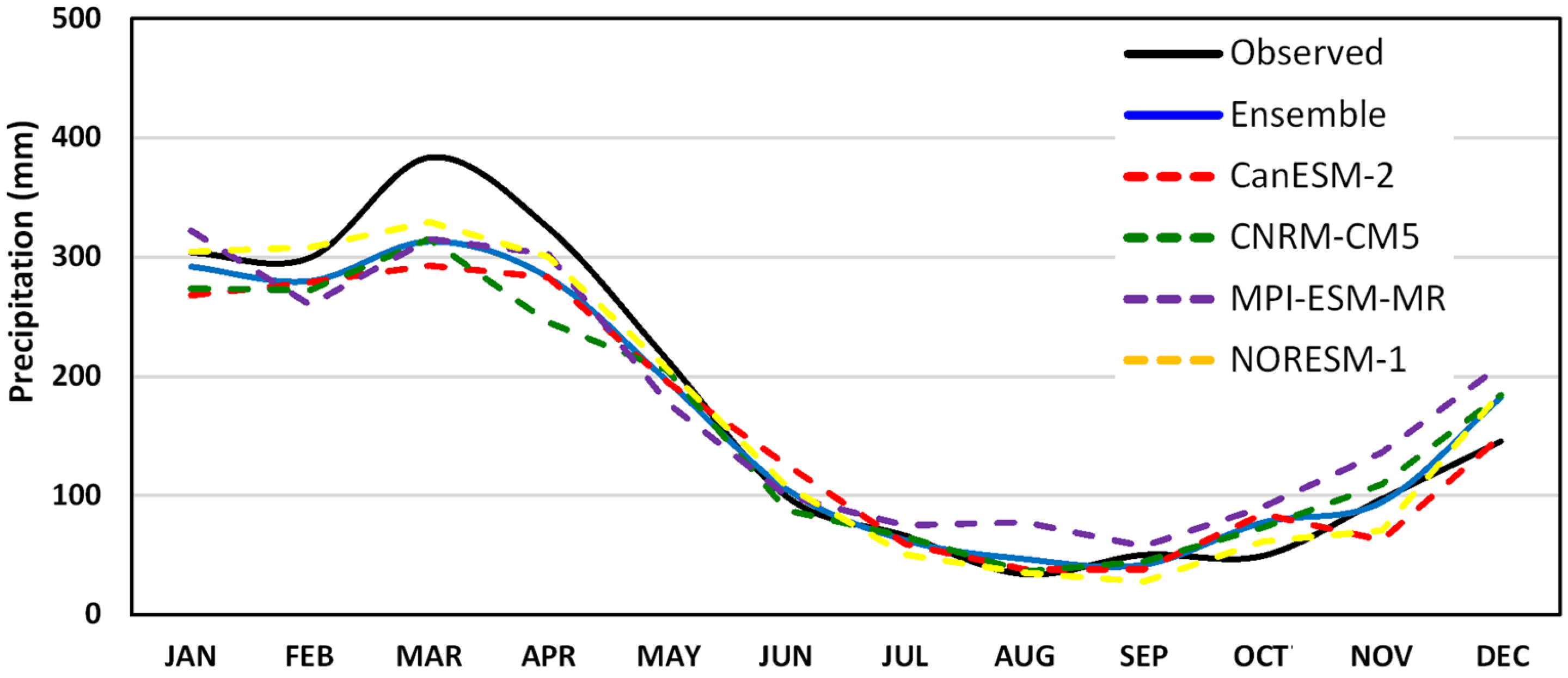
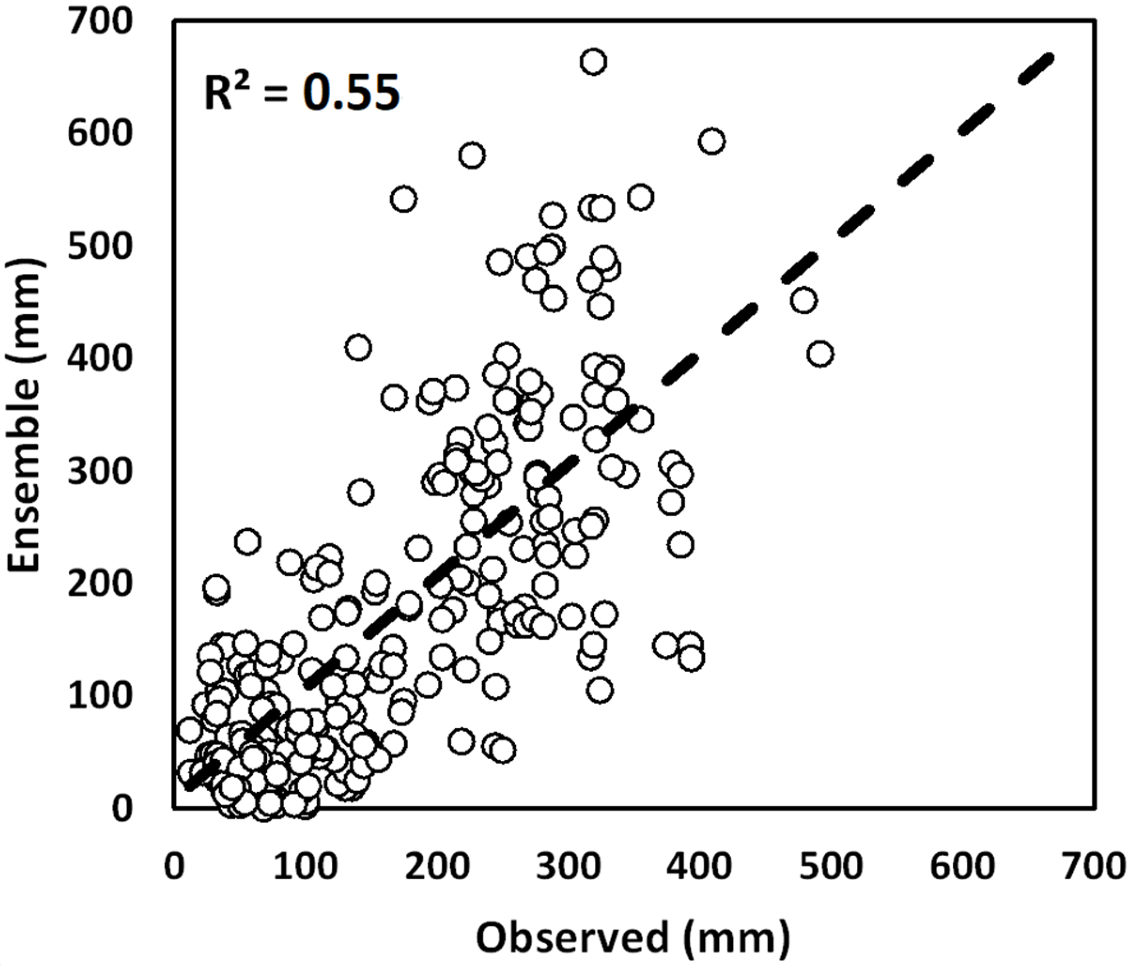
3.1. Statistical Downscaling Model Evaluations

The first step performed was to verify if the selected models were capable of satisfactorily representing the past climate. The period 1979–2010 was used for assessments of such scope. Figure 3 shows the results of simulations of monthly precipitation climatology by the four models and their ensemble for the grid point that corresponds to the Altamira station location, compared to observations from the same period. No considerable discrepancies between the simulations nor superiority of any one in particular was noticed. This ratified our option for the use of the ensemble rather than one of them. The display of the ensemble results concurrently to those from each of the models facilitates the statistical analysis and corroborates the application of the research [16].

As observed in Figure 3, the comparison between the monthly precipitation climatology according to observed data collected in Altamira in the period 1979–2010 and results of simulations by the models and their ensemble for the same place lead to the conclusion that the models represented satisfactorily the monthly precipitation there, except for March, when the models presented an underestimation of about 70 mm on average. Typically, peak amounts of rainfall are observed in March, with accumulations of almost 400 mm. For the dry period, the simulated monthly values were very close to the observations.

According to the scatter plot between the simulated monthly precipitation (ensemble) and the data recorded in Altamira for the training period 1979–2010 (Figure 4), the results with r = 0.75 and the coefficient of determination (R²) value of 0.55, indicate a strong correlation between simulated and observed data sets. BIAS presented a slight negative value (−6.51 mm) and RMSE was at 98.68 mm, mainly associated with the underestimation of the ensemble during the rainy season in Altamira.

The deviations of the simulations relative to the observations in the period 1979–2010 for the XRB are presented in Figure 5. The results show that, overall, the models tend to underestimate rainfall during the wet season, especially between February and April, with significant negative deviations in the north and west sectors. Better results are observed in the dry season, with lower absolute differences between the simulations and observations. This applies most noticeably to the period from May to August. These results indicate that the past climate, as assessed based on the reference period 1979–2010, was well represented by the models based on the predictors from reanalysis. Nonetheless, the monthly precipitation in the future scenarios was subjected to correction for each month through the bias removal technique addressed in Section 2.5.

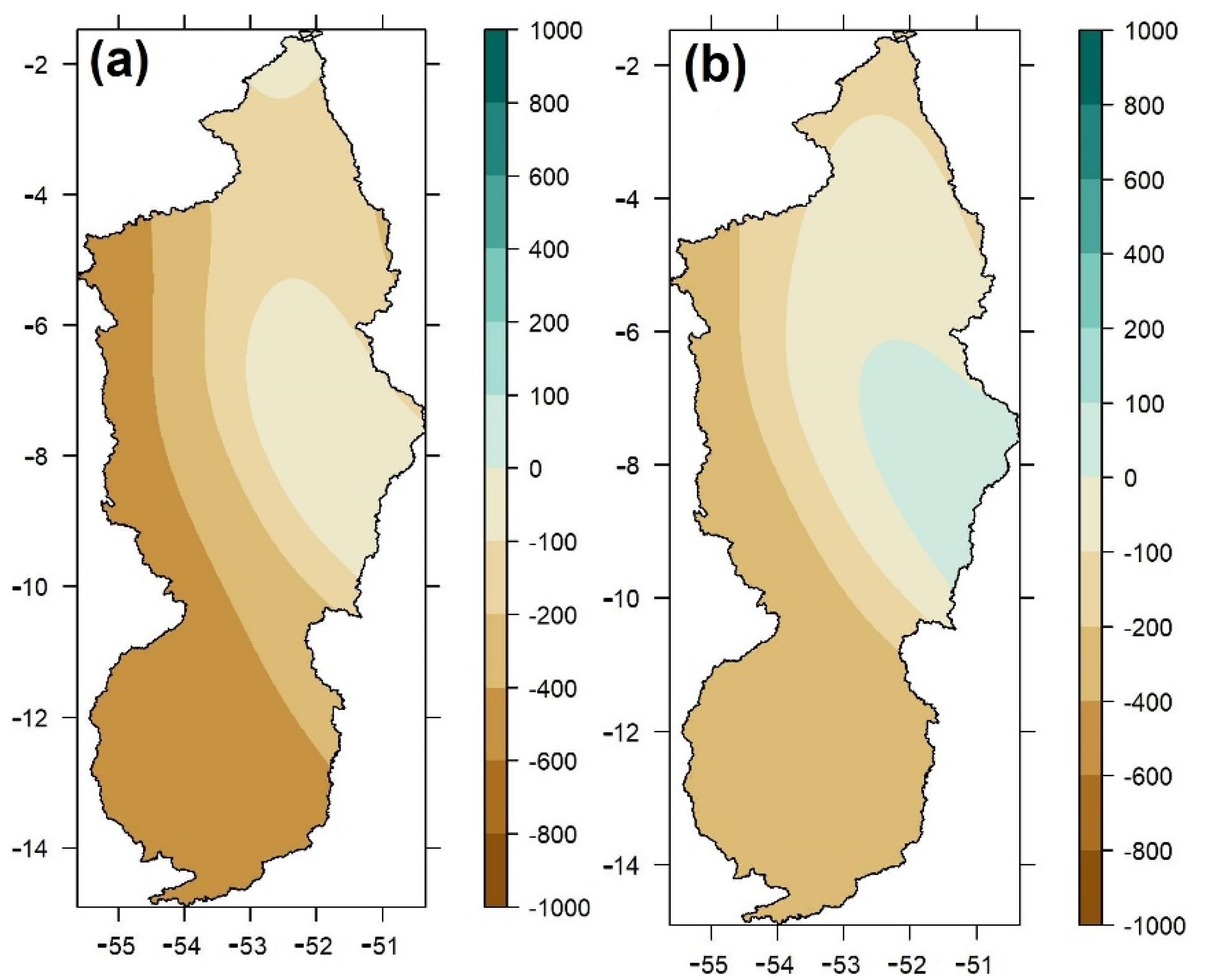
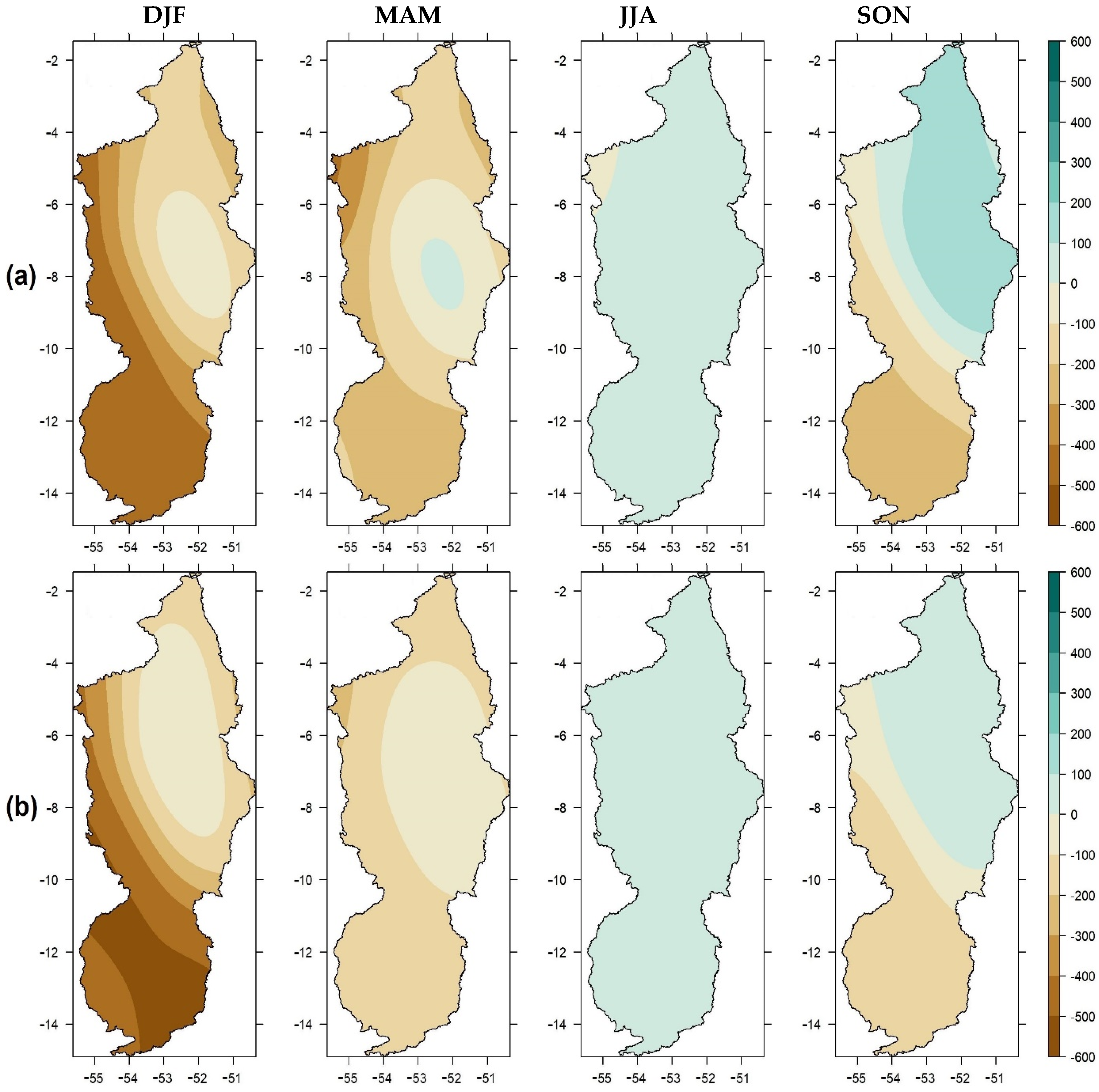
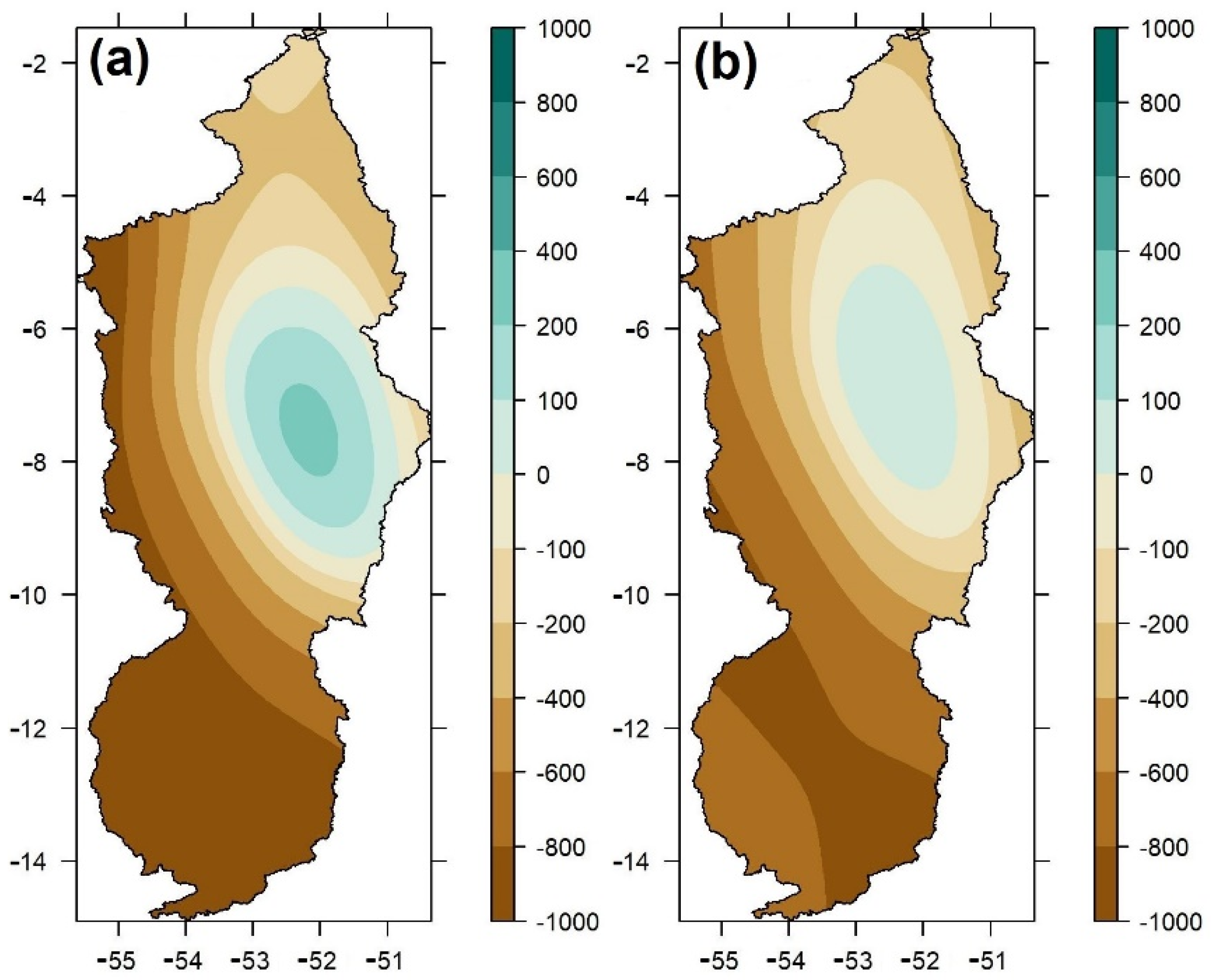
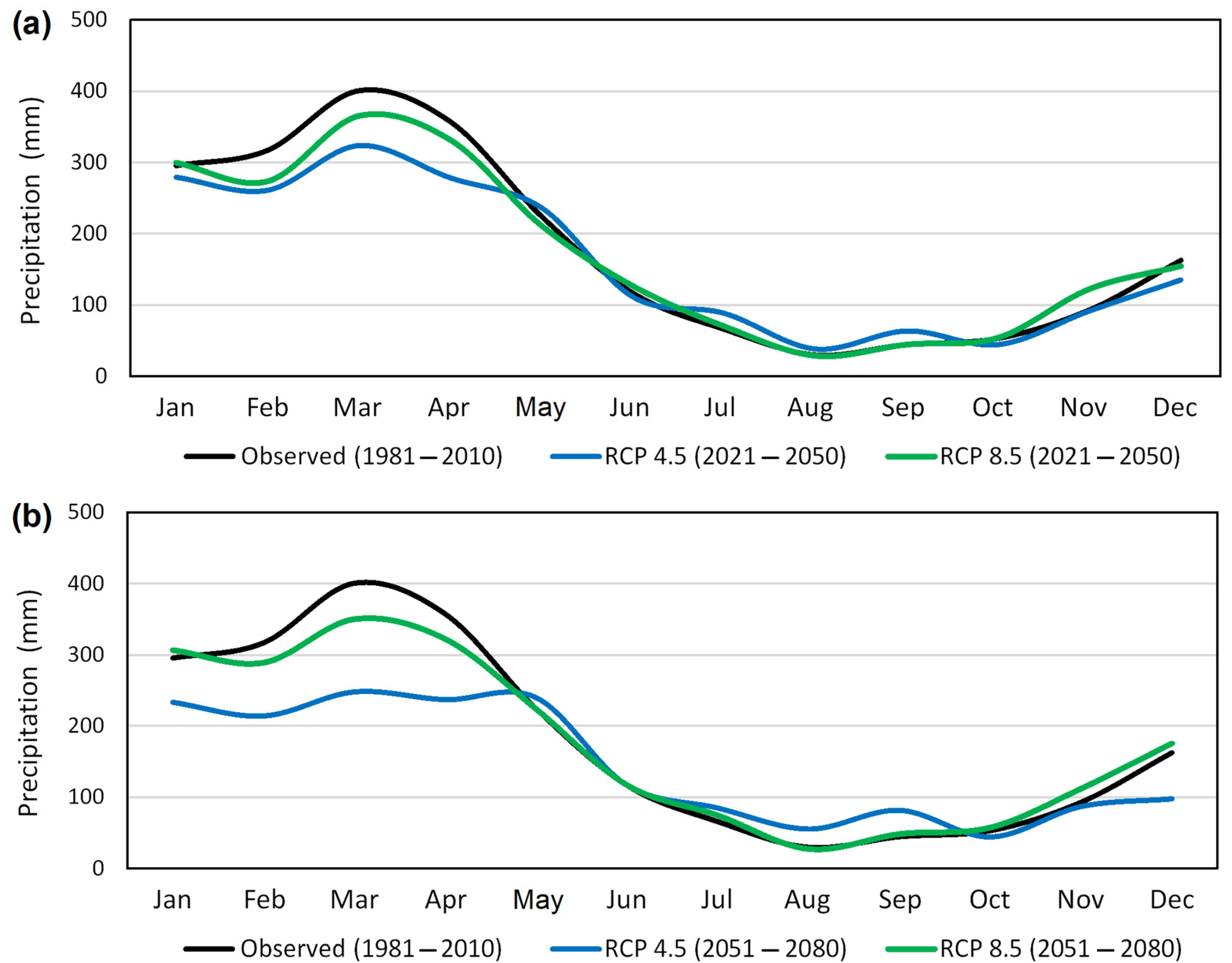
3.2. Climate Scenarios Applied to Precipitation

The climate projections based on the two different emission scenarios are applied to precipitation data with the ensemble of the models. The results of the precipitation simulations for the XRB based on the RCP 4.5 and RCP 8.5 scenarios are presented sequentially for two different 30-year periods, 2021–2050 (Figure 6 and Figure 7) and 2051–2080 (Figure 8 and Figure 9), which comprise two consecutive climatological normals. The projected seasonal deviations for precipitation over the XRB, in the period 2021–2050, in relation to the climatology of 1981–2010, as obtained through the ensemble of the models, are exhibited for both emission scenarios in Figure 6.

The spatial behavior of the deviations is similar in both scenarios, but with slightly lower magnitudes for the RCP 8.5. The DJF (summer) and MAM (autumn) quarters exhibit negative deviations, indicating an expected reduction in precipitation volumes, especially in the south and in the west. In JJA (winter), a slight increase in precipitation, of up to 100 mm, is to be expected nearly throughout the basin. For the SON (spring) quarter, the projections point to mild positive deviations in the north and to the east of the middle sector, whereas negative deviations are projected for the west and the south.

Figure 7 shows the annual deviation in precipitation between the average of the projections based on each of the scenarios and the reference period of 1981–2010. Both scenarios exhibit a similar behavior with regard to spatial pattern, indicating a reduction in the amount of precipitation for most of the XRB, with higher negative deviations in the south and western sectors (Upper and Middle Xingu), where the RCP 4.5 projects an annual deviation of more than 400 mm (Figure 7a). In the northern portion of the basin (Lower Xingu), the scenarios indicate negative annual deviations of up to 100 or 200 mm. For an area to the east of the center (the eastern part of Middle Xingu), the projections based on the RCP 4.5 suggest a decrease of less than 100 mm per year, whereas the RCP 8.5 signals an increase of up to 100 mm in the annual rainfall volume.

In Figure 8 and Figure 9, the seasonal and annual projected deviations, respectively, are exhibited for the period 2051–2080. Analogously to Figure 6, the spatial patterns are quite similar between the two emission scenarios. It is worth mentioning a substantial reduction in precipitation in DJF, especially in the south and along the western strip, which may experience a decrease of up to 500 mm for that quarter alone. Milder reductions are expected in the MAM quarter according to both scenarios. The JJA quarter should see a slight increase in precipitation, of up to 100 mm across the whole basin. In SON, a positive deviation is projected for the north and to the east of the center part, while negative amounts should be observed in the south and in the west, with slightly higher deviations being predicted based on the RCP 4.5 scenario. In general, projections according to both scenarios indicate a considerable reduction in rainfall during the wet season and mild increments in the dry season in the XRB for those three decades.

Regarding the annual deviations for the same period, higher numbers are projected for this period (Figure 9) than the first one (Figure 7). However, the spatial pattern is largely the same, suggesting a strong decrease in precipitation in southern XRB (Upper Xingu), where the RCP 4.5 scenario projections show negative deviations in excess of 800 mm. For this period, both scenarios indicate a slight increase in the rain over an area to the east of the center (eastern Middle Xingu). The projections based on the RCP 8.5 scenario are nearly the same for this region across both 30-year periods, whereas the ones based on the RCP 4.5 differ in which a negative deviation of less than 100 mm is indicated for 2021–2050, but a positive deviation of up to 200 mm is signaled for 2051–2080. The incongruent behavior of this area, by displaying projections of positive deviations while reductions are projected for most of the basin, may be associated with the application of the bias removal technique and/or reflect the quality of the data used for the reference period (observations from the station based at São Felix do Xingu, PA). For the northern sector (Lower Xingu), the projections are mostly the same as the ones for the previous period, with the exception of the westernmost part, where higher decreases are to be expected for this period.

Concerning the projections for Altamira, Figure 10 shows the monthly mean precipitation from the reference period and the projected numbers conforming to each of the emission scenarios for both the 30-year periods. An overall reduction in rainfall is expected during the wet season, most notably in the FMA quarter, with a slight decrease being projected for the dry season by both scenarios, especially from July to September, according to RCP 4.5, and in October and November, based on the RCP 8.5.

The monthly climatology of precipitation in the XRB was reflected in the results from both scenarios for the Altamira station for both periods.

Table 2. Deviations (%) in the projected precipitation for Altamira relative to the 1981–2010 period.

Scenarios	RCP 4.5		RCP 8.5
Period	2021–2050	2051–2080	2021–2050	2051–2080
DFJ	−12.9	−29.6	−6.1	−0.5
MAM	−14.6	−26.2	−7.5	−8.7
JJA	12.0	21.3	6.1	3.2
SON	4.5	11.7	15.8	14.3
ANNUAL	−9.7	−19.4	−3.6	−2.6

shows the expected variation, in percentage, in precipitation as measured at that station for each period, relative to the reference period of 1981–2010. Qualitatively, the seasonal behavior is similar across both scenarios, indicating a negative variation in the wet season (DJF and MAM quarters) and a positive variation in the dry one (JJA and SON). The annual variations were also of the same sign for both scenarios in both periods.

Nonetheless, the degree of variation according to one scenario differs considerably from the one projected through the other. For the nearest horizon (2021–2050), the RCP 4.5 and RCP 8.5 projections indicate an annual reduction of 9.7% and 3.6%, respectively. A higher discrepancy is observed in the projections for the 2051–2080 period, where the RCP 4.5 results in a much larger decrease (−19.4%) than the RCP 8.5 (−2.8%), even though it is the RCP 8.5 scenario that represents the most pessimistic future climate projections in the context of global warming, which leads to a radiative forcing of 8.5 W.m⁻² by 2100, as a consequence of a high rate of increase in the concentration of greenhouse gases in the atmosphere, especially carbon dioxide.

One of global warming projected impacts is alterations in the vegetation cover [69]. However, higher levels of carbon dioxide in the atmosphere can also favor plant growth [70], and some species are more tolerant and less sensible to environmental change than others [71].

This work did not directly address changes in land use and cover (the influence of deforestation on the XRB). Therefore, these factors are not considered in our projections of future precipitation, which leads us to conjecture that the lower amounts of precipitation decreases delivered by RCP 8.5 can be explained by that. Moreover, the most pessimistic scenarios are associated with more often occurrences of extreme events, which can be characterized by either an excess or a deficit in precipitation [15,72].

It is important to highlight that, even with the BIAS removal technique applied to the projections of monthly rainfall data, the models continued to indicate a significant reduction in the XRB, mainly for its southern part during the wet season. Most climate models predict less precipitation for the southeastern region of the Amazon, which includes the headwaters of the Xingu River [18,64]. These results are in agreement with previous works that performed CMIP5 simulations, which have also indicated an overall reduction in rainfall along the Amazon basin [7,8].

3.3. Projections of Future Flow Rates

In order to better understand the relationship between precipitation and flow rate at the XRB, the monthly climatology of those two variables, based on observed data at Altamira in the period 1981–2010 was plotted and exhibited in Figure 11, which shows a clearly identifiable rainfall regime. The region has a dry period from July through November, with the lowest amounts of precipitation being observed in the ASO quarter, when the monthly values typically fail to reach 50 mm, and a wet season from December through May, with the monthly precipitation exceeding 300 mm during the FMA quarter.

The monthly climatology of flow rate at Altamira follows a similar behavior to the one of precipitation, with the ebb period taking place from July to December and the flood period from January to June. As showcased in Figure 11, April presents the peak in flow rate, reaching about 20,000 m³s⁻¹, while September sees the lowest flow rate of the year, of only 1200 m³.s⁻¹. It is worth noting that the aforementioned peak in April happens in the month after the one when the peak in precipitation is observed, which is March. This evinces the relationship of dependence of the flow rate in one month (t) on the precipitation in the previous month (t − 1) for Altamira, especially during the wet season and the transition periods of December–January and May–June.

The monthly flow rates at the Altamira station were estimated using the PCR technique for the 2021–2050 and 2051–2080 periods based on the precipitation projections. Figure 12 shows the monthly mean flow according to the RCP 4.5 and RCP 8.5 scenarios for both future periods compared to the ensemble simulations for the reference period (1981–2010). In general, the projections reflect the ones for precipitation in Altamira for both periods, suggesting a considerable reduction during the flood period, especially in the FMA quarter, and a slight increase in the ebb period.

The projections from both scenarios for the 2021–2050 period (Figure 12a) show that the flow seasonality is preserved, with no changes being observed with respect to the month when the flow rate peaks (April) and the ones when it reaches its annual minimum (from September to October). Analogously to the precipitation projections, the RCP 4.5 scenario projects more prominent decreases than the RCP 8.5 for the flood period.

For the 2051–2080 period, the projections based on both scenarios (Figure 12b) denote a change in the month when the flow rate reaches its highest value. In consonance with the RCP 4.5 scenario, the peak should occur one month in advance (March) relative to the reference period (April), with a smooth decline taking place since then towards the ebb period, whereas, according to the RCP 8.5, a double peak scenario should happen, where the two maxima show up in March and May, with the latter being higher. April, however, exhibits similar values for the variable, so that the MAM quarter resembles a plateau. Such a behavior can be associated with factors such as bias removal in the precipitation projections and the delays that were applied to the simulation process of the rainfall–runoff model.

In Figure 13, the flow permanence curves of the monthly flow rates in Altamira are exhibited for both the future periods, where the reference curve is also plotted for comparison. The latter evinces that the flow rate in Altamira exhibits a large variability. This behavior is maintained in both scenarios, especially in 2021–2050. The greatest reductions take place from the point where the flow rate equals or exceeds Q40 up to when they reach Q5. The flow permanence curve suggests a trend of longer periods under the minimum flows. Q90 and Q95 (steady flow) should observe an increase in both periods according to both scenarios.

The monthly mean flow rate of 8114 m³s⁻¹ is equaled or surpassed in 39% of the time in 1981–2010. This average should be matched or exceeded in 2021–2050 in 38% and 42% of the time according to the projections based on the RCP 4.5 and on the RCP 8.5, respectively (Figure 13a). For the 2051–2080, it is projected that the average will be reached or exceeded in 36% of the time according to both pathways (Figure 13b). By comparing the flow permanence curves, it is evident that the 2021–2050 period shows peaks of higher amounts, whereas the 2051–2080 period suggests a lower variability regarding the projected monthly rates.

The percentage change of the projections for both future periods according to both pathways relative to the observed period of 1981–2010 are shown in

Table 3. Deviation (%) in the projected flow rate for Altamira relative to the 1981–2010 period.

Scenarios	RCP 4.5		RCP 8.5
Period	2021–2050	2051–2080	2021–2050	2051–2080
DFJ	−13.0	−15.4	−4.6	−15.0
MAM	−17.1	−31.6	−13.1	−22.4
JJA	3.9	12.6	4.8	1.0
SON	−5.8	−0.3	6.9	8.6
YEAR	−12.9	−20.2	−7.6	−16.0

for each quarter of the year. During the DJF and MAM quarters, the deviations based on both scenarios behave similarly, pointing to a decrease in the flow, mainly during the MAM quarter, which is the flood period. The negative deviation is highest for this season for the RCP 4.5 scenario, particularly in the 2051–2080 period. For the JJA quarter, the projections signal positive variations according to both scenarios, albeit slight, except for the 2051–2080 projection based on RCP 4.5, according to which the observed increase should reach the two digits. As for the SON quarter (the ebb season), the RCP 4.5 scenario indicates a mild decrease, whereas the RCP 8.5 suggests slightly positive variations for both periods.

Concerning the annual totals, both scenarios point to overall reductions in Altamira in both future periods. As in the precipitation results, the projected negative deviations reached higher amounts with the RCP 4.5 scenario than with the RCP 8.5. The projections indicate a lower annual reduction for the nearer horizon (2021–2050), of −12.9% and −7.6%, based on the RCP 4.5 and RCP 8.5, respectively, than for the more distant one (2051–2080), during which the negative variations may reach up to −20.2% and −16.0%, respectively (Table 3).

By coupling a GCM with a terrestrial ecosystem model (CCM3/IBIS), the projections by Ref. [63] suggest an overall decrease in the flow rate across XRB that varies from 6% to 36% depending on the deforestation scenario that is implemented for the Amazon basin. The said results are similar to the ones found here, which point to deviations in Altamira that vary between −12.9% and −7.6% for 2021–2050 according to the RCP 4.5 and RCP 8.5 emission scenarios, respectively.

Conforming to the Technical Note on the calculation of the “physical guarantee” of the BMHPP [64], for the Francis turbine in the main powerhouse (Belo Monte) to operate at its maximum capacity, a nominal flow of 775 m³s⁻¹ is required, although it can also operate safely, without risk of cavitation, at a partial load of 465 m³s⁻¹ (60% of the nominal flow). Based on the aforementioned specifications and considering that the BMHPP is of the run-of-the-river type, aimed at maintaining a fairly constant water level, the flow projections for Altamira under the effect of climate change warn that its main powerhouse may not be in operational conditions during the SON quarter (ebb season) for several years in both the assessed future periods.

3.4. Electricity Generation in Belo Monte

The energy generation potential at Belo Monte was estimated from the projections of flow rate at Altamira for the 2021–2050 and 2051–2080 periods based on both emission scenarios. Figure 14 shows a comparison between the generation potential estimations based on the flow rates of the reference period (1981–2010) with the projections. According to the projections of precipitation and flow rate, the results indicate a noteworthy decrease in the energy generation during the flood season and a slight increase in the ebb period for both scenarios.

One known characteristic of the energy generation at Belo Monte is that, from July to December (the ebb season), the projections cannot reach the guaranteed capacity in any of those months, staying under the value of 4419 MW that was estimated in its project. This pattern is maintained in all the projections presented here (for both periods, based on both scenarios).

With the exception of some months during the dry season, the RCP 4.5 pathway projections display higher decreases than the RCP 8.5 ones, but the monthly climatology of the governing variables is qualitatively reflected and sustained relative to the reference period. Conforming to the RCP 8.5 projections for 2051–2080, that period should see a shift of the generation peak from March to May, which reflects the change in the flow projections for the same period, although that is more conspicuous here.

The projections of generation potential at Belo Monte, relative to the maximum installed capacity of 11,000 MW, is displayed for each quarter of the year in

Table 4. Projections of generation potential (%) relative to the maximum installed capacity.

Scenarios	RCP 4.5		RCP 8.5
Period	2021–2050	2051–2080	2021–2050	2051–2080
DJF	46.4	44.9	51.6	45.1
MAM	69.1	56.4	78.9	67.7
JJA	19.0	21.2	19.6	18.0
SON	4.8	5.3	6.1	6.3
YEAR	38.8	31.6	39.1	34.3

. For DJF, the projections indicate a usage of 46.4–51.6% of the installed capacity during 2021–2050, and around 45% in 2051–2080. As expected, the best performance of the plant happens in MAM, with projections of 69.1% and 78.9% according to the RCP 4.5 and RCP 8.5 scenarios, respectively. In JJA, the performance should be around 20%, whereas, in the SON quarter, the usage should barely reach 5% for both periods, based on the RCP 4.5, and a little over 6% according to the RCP 8.5. In terms of annual generation, the two applied scenarios are very close in their projections for the 2021–2050 horizon, at about 39%, while, for the 2051–2080 period, there is a more considerable divergence of 2.7% between them, with the RCP 8.5 being the most optimistic.

Table 5. Variation (%) in the generation potential between the projections and the reference period (1981–2010).

Scenarios	RCP 4.5		RCP 8.5
Period	2021–2050	2051–2080	2021–2050	2051–2080
DJF	−12.9	−15.7	−3.2	−15.4
MAM	−21.3	−35.8	−10.2	−23.0
JJA	−10.1	−0.1	−7.3	−15.0
SON	−7.9	3.3	17.8	21.3
YEAR	−13.3	−21.3	−2.8	−14.7

shows the variation in the generation potential at Belo Monte that should be observed in the two analyzed periods according to the projections based on the two applied pathways relative to the reference period (simulated). In agreement with both scenarios, the DJF, MAM and JJA quarters should see a decrease in that variable, especially in MAM (flood period) in the 2051–2080 period, with reductions varying from −23.0% to −35.8%. The only variations of a positive sign are found in the SON. For this quarter, the RCP 8.5 scenario projects prominent increases for both periods, reaching 21.3% in the 2051–2080 period.

Overall, the projections based on both climate scenarios suggest a decrease in the energy generated at Belo Monte in both future periods. For the nearer horizon (2021–2050), annual reductions of −13.3% and −2.8% are projected through the RCP 4.5 and RCP 8.5, respectively. More noticeable declines are expected on the farther horizon (2051–2080), for which the projections signal variations of −21.3% (RCP 4.5) and −14.7% (RCP 8.5).

Figure 15 summarizes the projections of precipitation, flow rate and energy generation for both future periods relative to the observations in 1981–2010. In general, the results point to a decrease in precipitation and river flow rate in Altamira, and, consequently, in the electricity generation at Belo Monte. The reductions based on the RCP 4.5 scenario (Figure 15a) are more prominent than those accomplished through the application of the RCP 8.5 (Figure 15b), with the difference being higher in the 2021–2050 period (Figure 15a).

4. Discussion

The above results indicate that less precipitation and river flow rate are to be expected in Altamira in the future, affecting the electricity generation at Belo Monte in the two analyzed periods, which correspond to most of the remainder of this century. The most worrying situation concerns the period of 2051–2080, for which the monthly mean generation estimate does not even reach 8000 MW (Figure 14), thus staying considerably under the maximum installed capacity of the plant, which is 11,000 MW. These results strengthen the debate regarding the efficiency and performance of the BMHPP in the future [64].

Ref. [73] simulated precipitation and flow rate for the Amazon basin for the 2050 horizon by coupling a GCM with a terrestrial ecosystem model (CCM3/IBIS) considering two scenarios: one where a “strict governance” on deforestation takes place and another called “business-as-usual”, which represents a continuation of deforestation activities without proper surveillance and legal limits. In regard to precipitation, both scenarios pointed to a decrease throughout the basin. The results for the XRB indicated a reduction of 15% for the scenario where deforestation is kept under control and of 20% for the uncontrolled deforestation scenario. As for flow rate, the work by Ref. [73] signals a reduction of 11% for the regulated deforestation scenario and of 17% for the generalized deforestation prospect. Ref. [64] also examined the effects of deforestation in the river flow rate and energy generation at Belo Monte. According to these authors, the deforestation in the Amazon region would reduce precipitation and flow rate by 6–36% based on different deforestation scenarios. Conforming to their “business-as-usual” scenario, assuming a forest loss of 40% until 2050, the projected energy generation would drop to a mere 25% of the maximum capacity and 40% of the estimates in the plant project. Although our work employs scenarios of different warming forcings, rather than deforestation levels, the sign and degree of the projected precipitation and flow rate deviations for the XRB in our findings are close to the ones of those studies, especially for the 2021–2050 horizon, which is disquieting, since both the deforestation and the general warming scenarios can combine and lead to a troublesome future.

The combined impacts of land use and cover change and of warming climate scenarios (RCP 4.5 and RCP 8.5) have been addressed by Ref. [74], for the Tapajós basin in the Brazilian Amazon. The results for the 2026–2045 period suggest that climate change may reduce the flow rate at the analyzed stations by up to 20% and that interannual variability may be increased. Concerning water resources management, the overall reduction in the rivers and the growing variability, combined with the alteration and shortening of the wet season, may considerably affect the productivity of major hydropower systems that are being planned for the region.

A more recent study on the flow trends observed in the past decades along the Amazon basin revealed substantial variations, of ± 9.5 mm/year, for the whole basin [75]. The changes, however, presented a characteristic spatial pattern across the basin, through which the north and west sectors experienced an increase in the flow rates, whereas the south and the east, including the XRB, have seen a negative trend.

Pertaining to some of the techniques employed here, the findings of Ref. [22], with emphasis on the reference station at Altamira, as in our results, also attest the satisfactory performance of the PCR technique when applied to simulate monthly mean flows in the XRB. In fact, the application of PCR for rainfall–runoff modeling meets a demand for less complex, faster and yet reliable forecasts, especially in large basins such as the ones across the Amazon, with problems of availability of input data for conceptual models. The technique, therefore, can be regarded as a useful and operational tool for simulating monthly flows along the XRB. Monthly flow rate forecasts using this technique can be achieved from seasonal climate predictions and/or future climate scenarios.

Some works have also assessed the expected energy production of the Brazilian Hydropower generation systems for the remainder of this century in view of different climate change scenarios, for several production regions across the country: Xingu [64], Tocantins [76]; Tapajós [77], Madeira [78], and São Francisco [79,80]. These studies projected a strong reduction in precipitation in the North and Northeast regions of Brazil, with an appreciable decrease in the generation potential of the systems hosted by them, which include important power plants, such as Belo Monte, Tucuruí, Teles Pires, Jirau, and Xingó.

Ref. [78] investigated the impact of climate change on the hydropower planet of Tucuruí in the 2011–2070 horizon. Their findings project a reduction from 27% to 56% on the generation potential, according to the different scenarios. That facility has an installed capacity of 8370 MW, exerting an important role in terms of contribution to the national energy production of the country. In fact, the systems located in the North and Northeast regions represent 20.5 and 21.3% of the installed potential of Brazil [1].

Conversely, future projections of energy production at the systems of the South indicate that climate change might be beneficial for them in this regard until the end of the century, since a significant increase is expected according to the scenarios assessed by Ref. [6]. Precipitation projections by Ref. [81] considering the RCP 4.5 scenario for the 2011–2099 horizon along the Plata basin indicate a positive trend for southern Brazil and northern Argentina from 2041, which favors hydropower generation in those regions, corroborating the aforementioned findings of Ref. [6]. The systems in the South of Brazil represent 19% of the installed national potential [1] and include the largest hydropower plant in the country, the “Itaipu Binacional”.

In general, studies assessing the feasibility of hydropower facilities do not take into consideration the effects of climate change in their planning. Some works, however, have discussed the current situation, future perspectives and impacts of climate change on the existing Brazilian reservoirs [2,5]. Investments in other renewable energy sources, such as solar, wind and biomass, are needed in order to compensate for the expected losses in the hydropower production [79] and to guarantee a more stable and robust energy portfolio [6].

5. Conclusions

The SDM employed here was efficient in simulating the monthly precipitation series for the past reference period in the XRB. The results presented satisfactory values for the skill indices for the simulations performed by the ensemble of the four adopted GCMs considering the observed amounts in the reference period. On the whole, they represented very well the dynamic of monthly precipitation, with some underestimation in the wet season (especially in March–April) and a slight overestimation in the dry period.

As for the projections for the future in Altamira, based on both the RCP 4.5 and RCP 8.5 scenarios, a decrease in precipitation is envisioned for 2021–2080 relative to the reference period (1981–2010). As expected, the flow rate projections also exhibit negative deviations for the same period, reflecting the reduction in rainfall for both the 30-year segments (2021–2050 and 2051–2080). As a consequence, the energy generation potential at Belo Monte is also predicted to fall. The RCP 4.5 scenario resulted in lower precipitation and flow rate reductions, when compared to the RCP 8.5. According to the latter, a reduction of 21.3% in the annual generation potential at the BMHPP is expected until 2080, with a corresponding use of 38.8% of the maximum installed potential.

Climate change may also influence the level of severity of extreme events in the upcoming decades, such as floods and droughts. The XRB region has been under pressure from agribusiness and the forced advance of agriculture and livestock frontiers around it, which leads to an increase in the demand for water resources in order to meet the multiple activities taking place along the basin. These factors, combined with climate change, might influence water availability for hydropower generation at Belo Monte. The BMHPP managers and government decision makers can use information provided by studies such as this to adopt energy regulations and measures towards the mitigation of possible impacts of such scenarios.

Since the BMHPP reservoir is of the run-of-the-river type, aimed at maintaining a fairly constant water level, it cannot rely on a reservoir big enough to maintain a high generation potential during the dry period, thus depending solely on the natural variability of the Xingu River. This characteristic aggravates its vulnerability to extreme climate events and hinders the ability to adjust the water level, with the largest flow rates being limited in time to only four months per year (FMAM). The findings presented here emphasize the need for taking into consideration climate projections in the planning of hydroelectric facilities of this type.

The presented results also highlight the need for reducing the dependency of Brazil on hydroelectricity while also avoiding having to rely on thermal (fossil) energy in times of shortages by diversifying the nation’s portfolio towards renewable energy sources other than hydropower, such as wind and solar, in order to increase the national energy security and compensate for the upcoming losses in hydroelectricity production at Belo Monte.

The results obtained in this research will also serve as a basis for the calibration and verification of the Brazilian Global Atmospheric Model (BAM) [82], which is the atmospheric module of the Brazilian Earth System Model (BESM), in order to adjust the surface data estimates to weather forecasting purposes for the XRB.

References

1. EPE—Empresa de Pesquisa Energética. Anuário Estatístico de Energia Elétrica. 2020. Available online: http://www.epe.gov.br (accessed on 5 March 2021).
2. De Souza Dias, V.; Pereira da Luz, M.; Medero, G.M.; Tarley Ferreira Nascimento, D. An Overview of Hydropower Reservoirs in Brazil: Current Situation, Future Perspectives and Impacts of Climate Change. Water 2018, 10, 592. [Google Scholar] [CrossRef] [Green Version]
3. De Menezes, J.B.; Bandeira, O.M.; Leite, D.T. A construção do complexo hidrelétrico de Belo Monte: Quarta maior do mundo em capacidade instalada. Rev. Bras. Eng. Barragens 2017, 4, 5–21. [Google Scholar]
4. Norte Energia. UHE Belo Monte, a Maior Usina Hidrelétrica 100% Brasileira. Brasília. Available online: https://www.norteenergiasa.com.br/pt-br/uhe-belo-monte/a-usina (accessed on 20 March 2021).
5. Mendes, C.A.B.; Beluco, A.; Canales, F.C. Some important uncertainties related to climate change in projections for the Brazilian hydropower expansion in the Amazon. Energy 2017, 141, 123–138. [Google Scholar] [CrossRef]
6. De Queiroz, A.R.; Faria, V.A.D.; Lima, L.M.M.; Lima, J.W. Hydropower revenues under the threat of climate change in Brazil. Renew. Energy 2019, 133, 873–882. [Google Scholar] [CrossRef]
7. Chou, S.C.; Lyra, A.; Mourão, C.; Dereczynski, C.; Pilotto, I.; Gomes, J.; Bustamante, J.; Tavares, P.; Silva, A.; Rodrigues, D.; et al. Assessment of Climate Change over South America under RCP 4.5 and 8.5 Downscaling Scenarios. Am. J. Clim. Chang. 2014, 3, 512–525. [Google Scholar] [CrossRef] [Green Version]
8. Martins, G.; Von Randow, C.; Sampaio, G.; Dolman, A.J. Precipitation in the Amazon and its relationship with moisture transport and tropical Pacific and Atlantic SST from the CMIP5 simulation. Hydrol. Earth Syst. Sci. 2015, 12, 671–704. [Google Scholar]
9. Woldemeskel, F.M.; Sharma, A.; Sivakumar, B.; Mehrotra, R. An error estimation method for precipitation and temperature projections for future climates. J. Geophys. Res. Atmos. 2012, 117, D22. [Google Scholar] [CrossRef]
10. Addor, N.; Seibert, J. Bias correction for hydrological impact studies—Beyond the daily perspective. Hydrol. Process. 2014, 28, 4823–4828. [Google Scholar] [CrossRef]
11. Hakala, K.; Addor, N.; Teutschbein, C.; Vis, M.; Dakhlaoui, H.; Seibert, J. Hydrological Modeling of Climate Change Impacts. In Encyclopedia of Water: Science, Technology, and Society; Wiley: Hoboken, NJ, USA, 2019; pp. 1–20. [Google Scholar] [CrossRef]
12. Meresa, H.K.; Romanowicz, R.J. The critical role of uncertainty in projections of hydrological extremes. Hydrol. Earth Syst. Sci. 2017, 21, 4245–4258. [Google Scholar] [CrossRef] [Green Version]
13. Kundzewicz, Z.W.; Krysanova, V.; Benestad, R.E.; Hov, O.; Piniewski, M.; Otto, I.M. Uncertainty in climate change impacts on water resources. Environ. Sci. Policy 2018, 79, 1–8. [Google Scholar] [CrossRef]
14. Hattermann, F.F.; Vetter, T.; Breuer, L.; Su, B.; Daggupati, P.; Donnelly, C.; Fekete, B.; Flörke, F.; Gosling, S.N.; Hoffmann, P.; et al. Sources of uncertainty in hydrological climate impact assessment: A cross-scale study. Environ. Res. Lett. 2018, 13, 015006. [Google Scholar] [CrossRef]
15. Dos Santos, D.J.; Pedra, G.U.; Da Silva, M.G.B.; Junior, C.A.G.; Alves, L.M.; Sampaio, G.; Marengo, J.A. Future rainfall and temperature changes in Brazil under global warming levels of 1.5 °C, 2 °C and 4 °C. Sustain. Debate 2020, 11, 57–73. [Google Scholar] [CrossRef]
16. De Moura, C.N.; Seibertb, J.; Mine, M.R.M. Uncertainties in Projected Rainfall over Brazil: The Role of Climate Model, Bias Correction and Emission Scenario. California Digital Library. 2020. Available online: https://www.sciencegate.app/document/10.31223/osf.io/2p9wg (accessed on 20 July 2022).
17. Yin, L.; Fu, R.; Shevliakova, E.; Dickson, R.E. How well can CMIP5 simulate precipitation and its controlling processes over tropical South America? Clim. Dyn. 2013, 41, 3127–3143. [Google Scholar] [CrossRef] [Green Version]
18. Guimberteau, M.; Ronchail, J.; Espinoza, J.C.; Lengaigne, M.; Sultan, B.; Polcher, J.; Drapeau, G.; Guyot, J.-L.; Ducharne, A.; Ciais, P. Future changes in precipitation and impacts on extreme streamflow over Amazonian sub-basins. Environ. Res. Lett. 2013, 8, 014035. [Google Scholar] [CrossRef]
19. De Oliveira, B.F.A.; Bottino, M.J.; Nobre, P.; Nobre, C. Deforestation and climate change are projected to increase heat stress risk in the Brazilian Amazon. Commun. Earth Environ. 2021, 2, 207. [Google Scholar] [CrossRef]
20. Joetzjer, E.; Douville, H.; Delire, C.; Ciais, P. Present-day and future Amazonian precipitation in global climate models: CMIP5 versus CMIP3. Clim. Dyn. 2013, 41, 2921–2936. [Google Scholar] [CrossRef]
21. Silva, J.P.; Pereira, D.I.; Aguiar, A.M.; Rodrigues, C. Geodiversity assessment of the Xingu drainage basin. J. Maps 2013, 9, 254–262. [Google Scholar] [CrossRef] [Green Version]
22. Lucas, E.W.M.; Sousa, F.A.S.; Silva, F.D.S.; Rocha-Júnior, R.L.; Pinto, D.D.C.; Da Silva, V.P.R. Trends in climate extreme assessed in the Xingu river basin—Brazilian Amazon. Weather Clim. Extrem. 2021, 31, 10036. [Google Scholar] [CrossRef]
23. Schwartzman, S.; Vilas-Boas, A.; Ono, K.Y.; Fonseca, M.G.; Doblas, J.; Zimmerman, B.; Junqueira, P.; Jerozolimski, A.; Salazar, M.; Junqueira, R.P.; et al. The natural and social history of the indigenous lands and protected areas corridor of the Xingu River basin. Philos. Trans. 2013, 368, 20120164. [Google Scholar] [CrossRef] [Green Version]
24. De Oliveira, G.; Chen, J.M.; Mataveli, G.A.V.; Chaves, M.E.D.; Rao, J.; Sternberg, M.; Dos Santos, T.V.; Dos Santos, C.A.C. Evapotranspiration and Precipitation over Pasture and Soybean Areas in the Xingu River Basin, an Expanding Amazonian Agricultural Frontier. Agronomy 2020, 10, 1112. [Google Scholar] [CrossRef]
25. Reboita, M.S.; Gan, M.A.; Da Rocha, R.P.; Ambrizzi, T. Regimes de precipitação na América do Sul: Uma revisão bibliográfica. Rev. Bras. Meteorol. 2010, 25, 185–204. [Google Scholar] [CrossRef]
26. Dos Santos, C.A.; Lima, A.M.M.; Franco, V.S.; Araújo, I.B.; Menezes, J.F.G.; Gomes, N.M.O. Distribuição espacial da precipitação na bacia hidrográfica do rio Xingu. Nucleus 2016, 13, 223–230. [Google Scholar] [CrossRef] [Green Version]
27. De Azambuja, A.M.S. Climatologia da Precipitação na Bacia Hidrográfica do Rio Xingu; CPRM—Serviço Geológico do Brasil: Rio de Janeiro, Brazil, 2018. [Google Scholar]
28. ANA—Agencia Nacional de Aguas. Plano Estratégico de Recursos Hídricos dos Afluentes da Margem Direita do rio Amazonas: Diagnóstico; ANA—Agencia Nacional de Aguas: Brasilia, Brazil, 2013. [Google Scholar]
29. IPCC—Intergovernamental Panel on Climate Change. AR5 Climate Change 2014: Mitigation of Climate Change; Working Group III Contribution to the Fifth Assessment Report of the Intergovernmental Panel on Climate Change; Cambridge University Press: Cambridge, UK, 2014. [Google Scholar]
30. Moss, R.H.; Edmonds, J.A.; Hibbard, K.A.; Manning, M.R.; Rose, S.K.; Van Vuuren, D.P.; Carter, T.R.; Emori, S.; Kainuma, M.; Kram, T.; et al. The next generation of scenarios for climate change research and assessment. Nature 2010, 463, 747–756. [Google Scholar] [CrossRef]
31. Van Vuuren, D.P.; Edmonds, J.; Kainuma, M.; Riahi, K.; Thomsom, A.; Hibbard, K.; Hurtt, G.C.; Kram, T.; Krey, V.; Lamarque, J.-L.; et al. The representative concentration pathways: An overview. Clim. Chang. 2011, 109, 5–31. [Google Scholar] [CrossRef]
32. Taylor, K.E.; Stouffer, R.J.; Meehl, G.A. An overview of CMIP5 and the experiment design. Bull. Am. Meteorol. Soc. 2012, 93, 485–498. [Google Scholar] [CrossRef] [Green Version]
33. Arora, V.K.; Boer, G.J.; Christian, J.R.; Curry, C.L.; Denman, K.L.; Zahariev, K.; Flato, G.M.; Scinocca, J.F.; Merryfield, W.J.; Lee, W.G. The effect of terrestrial photosynthesis down-regulation on the 20th century carbon budget simulated with the CCCma earth system model. J. Clim. 2009, 22, 6066–6088. [Google Scholar] [CrossRef]
34. Christian, J.R.; Arora, V.K.; Boer, G.J.; Curry, C.L.; Zahariev, K.; Denman, K.L.; Flato, G.M.; Lee, W.G.; Merryfield, W.J.; Roulet, N.T.; et al. The global carbon cycle in the Canadian Earth system model CanESM1: Preindustrial control simulation. J. Geophys. Res. 2010, 115, G03014. [Google Scholar] [CrossRef] [Green Version]
35. Salas-Mélia, D.; Chauvin, F.; Déqué, M.; Douville, H.; Gueremy, J.F.; Marquet, P.F.; Planton, S.; Royer, J.F.; Tyteca, S. Description and Validation of the CNRM-CM3 Global Coupled Model; CNRM Technical Report; Centre National de Recherches Meteorologiques: Toulouse, France, 2005; 103p. [Google Scholar]
36. Voldoire, A.; Sanchez-Gomez, E.; Salas y Mélia, D.; Decharme, B.; Cassou, C.; Sénési, S.S.; Valcke, S.; Beau, I.; Alias, A.; Chevallier, M.; et al. The CNRM-CM5.1 global climate model: Description and basic evaluation. Clim. Dyn. 2011, 40, 2091–2121. [Google Scholar] [CrossRef] [Green Version]
37. Giorgetta, M.; Jungclaus, J.; Reick, C.; Legutke, S.; Bader, J.; Böttinger, M.; Brovkin, V.; Crueger, T.; Esch, M.; Fieg, K.; et al. Climate and carbon cycle changes from 1850 to 2100 in MPI-ESM simulations for the coupled model intercomparison project phase 5. J. Adv. Model. Earth Syst. 2013, 5, 572–597. [Google Scholar] [CrossRef]
38. Müller, W.; Jungclaus, J.; Mauritsen, T.; Baehr, J.; Bittner, M.; Budich, R.; Bunzel, F.; Esch, M.; Ghosh, R.; Haak, H.; et al. A higher-resolution version of the Max Planck Institute Earth System Model (MPI-ESM 1.2—HR). J. Adv. Model. Earth Syst. 2018, 10, 1383–1413. [Google Scholar] [CrossRef]
39. Bentsen, M.; Bethke, I.; Debernard, J.B.; Iversen, T.; Kirkevag, A.; Seland, O.; Drange, H.; Roelandt, C.; Seierstad, I.A.; Hoose, C.; et al. The Norwegian Earth System Model, NorESM1-M—Part 1: Description and basic evaluation of the physical climate. Geosci. Model Dev. 2013, 6, 687–720. [Google Scholar] [CrossRef]
40. Guo, C.; Bentsen, M.; Bethke, I.; Ilicak, M.; Tjiputra, J.; Toniazzo, T.; Schwinger, J.; Ottera, O.H. Description and evaluation of NorESM1-F: A fast version of the Norwegian Earth System Model (NorESM). Geosci. Model Dev. 2019, 12, 343–362. [Google Scholar] [CrossRef] [Green Version]
41. Wilby, R.L.; Charles, S.P.; Zorita, E.; Timbal, B.; Whetton, P.; Mearns, L.O. Guidelines for Use of Climate Scenarios Developed from Statistical Downscaling Methods. 2004. Available online: http://ipcc-ddc.cru.uea.ac.uk/guidelines/dgm_no2_v1_09_2004.pdf (accessed on 20 July 2021).
42. Silva, F.D.S.; Costa, R.L.; Da Rocha Júnior, R.L.; Gomes, H.B.; Azevedo, P.V.; Silva, V.P.R.; Monteiro, L.A. Cenários Climáticos e Produtividade do Algodão no Nordeste do Brasil. Parte II: Simulação Para 2020 a 2080. Rev. Bras. Meteorol. 2021, 35, 913–929. [Google Scholar] [CrossRef]
43. Fowler, H.J.; Blenkinsop, S.; Tebaldi, C. Linking climate change modelling to impacts studies: Recent advances in downscaling techniques for hydrological modelling. Int. J. Climatol. 2007, 27, 1547–1578. [Google Scholar] [CrossRef]
44. Dee, D.P.; Uppala, S.M.; Simmons, A.J.; Berrisford, P.; Poli, P.; Kobayashi, S.; Andrae, U.; Balmaseda, M.A.; Balsamo, G.; Bauer, P.; et al. The ERA-Interim reanalysis: Configuration and performance of the data assimilation system. Q. J. R. Meteorol. Soc. 2011, 137, 553–597. [Google Scholar] [CrossRef]
45. Gutiérrez, J.M.; San-Martin, D.; Brands, S.; Manzanas, R.; Herrera, S. Reassessing statistical downscaling techniques for their robust application under climate change conditions. J. Clim. 2013, 26, 171–188. [Google Scholar] [CrossRef] [Green Version]
46. Costa, R.L.; Gomes, H.B.; Silva, F.D.S.; Baptista, G.M.M.; Da Rocha Júnior, R.L.; Herdies, D.L.; Silva, V.P.R. Cenários de Mudanças Climáticas para a Região Nordeste do Brasil por meio da Técnica de Downscaling Estatístico. Rev. Bras. Meteorol. 2021, 35, 785–801. [Google Scholar] [CrossRef]
47. Costa, R.L.; Baptista, G.M.M.; Gomes, H.B.; Silva, F.D.S.; Da Rocha Júnior, R.L.; Nedel, A.S. Analysis of future climate scenarios for northeastern Brazil and implications for human thermal comfort. An. Acad. Bras. Ciênc. 2021, 93, 1–23. [Google Scholar] [CrossRef]
48. Ramírez, M.C.V.; Ferreira, N.J.; Velho, H.F.C. Linear and nonlinear statistical downscaling for rainfall forecasting over Southeastern Brazil. Weather Forecast. 2006, 21, 969–989. [Google Scholar] [CrossRef]
49. Hertig, E.; Maraun, D.; Bartholy, J.; Pongracz, R.; Vrac, M.; Mares, I.; Gutiérrez, J.M.; Wibig, J.; Casanueva, A. Comparison of statistical downscaling methods with respect to extreme events over Europe: Validation results from the perfect predictor experiment of the COST Action VALUE. Int. J. Climatol. 2018, 39, 3846–3867. [Google Scholar] [CrossRef]
50. Zorita, E.; Storch, H.V. The analog method as a simple Statistical Downscaling Technique: Comparison with more complicated methods. J. Clim. 1999, 12, 2474–2489. [Google Scholar] [CrossRef]
51. Chen, J.; Brissette, F.P.; Chaumont, D.; Braun, M. Finding appropriate bias correction methods in downscaling precipitation for hydrologic impact studies over North America. Water Resour. Res. 2013, 49, 4187–4205. [Google Scholar] [CrossRef]
52. Lenderink, G.; Buishand, A.; Deursen, W. Estimates of future discharges of the river Rhine using two scenario methodologies: Direct versus delta approach. Hydrol. Earth Syst. Sci. 2007, 11, 1145–1159. [Google Scholar] [CrossRef]
53. Kendall, M.G. Rank Correlation Methods; Charles Griffin: London, UK, 1975; 120p. [Google Scholar]
54. Hotelling, H. The relations of the newer multivariate statistical methods to factor analysis. Br. J. Math. Stat. Psychol. 1957, 10, 69–79. [Google Scholar] [CrossRef]
55. Rencher, A.C. Methods of Multivariate Analysis, 2nd ed.; Brigham Young University: Provo, UT, USA; Wiley: Hoboken, NJ, USA, 2002; 737p. [Google Scholar]
56. Izenman, A.J. Modern Multivariate Statistical Techniques; Springer: Berlin, Germany, 2008. [Google Scholar]
57. Lucas, E.W.M.; Sousa, F.A.S.; Silva, F.D.S.; Da Rocha Júnior, R.L.; Ataíde, K.R.P. Previsões de vazões mensais na bacia hidrográfica do Xingu—Leste da Amazônia. Rev. Bras. Meteorol. 2020, 35, 1045–1056. [Google Scholar] [CrossRef]
58. IRI—International Research Institute for Climate and Society. The Climate Predictability Tool. 2019. Available online: https://iri.columbia.edu/our-expertise/climate/tools/cpt/ (accessed on 15 August 2019).
59. Lucio, P.S.; Silva, F.D.S.; Fortes, L.T.G.; Santos, L.A.R.; Ferreira, D.B.; Salvador, M.A.; Balbino, H.T.; Sarmanho, G.F.; dos Santos, L.S.F.C.; Lucas, E.W.M.; et al. Um modelo estocástico combinado de previsão sazonal para a precipitação no Brasil. Rev. Bras. Meteorol. 2010, 25, 70–87. [Google Scholar] [CrossRef]
60. Kipkogei, O.; Mwanthi, A.M.; Mwesigwa, J.B.; Atheru, Z.K.K.; Wanzala, M.A.; Artan, G. Improved Seasonal Prediction of Rainfall over East Africa for Application in Agriculture: Statistical Downscaling of CFSv2 and GFDL-FLOR. J. Appl. Meteorol. Climatol. 2017, 56, 3229–3243. [Google Scholar] [CrossRef]
61. Esquivel, A.; Llanos-Herrera, L.; Agudelo, D.; Prager, S.D.; Fernandes, K.; Rojas, A.; Valencia, J.J.; Ramirez-Villegas, J. Predictability of seasonal precipitation across major crop growing areas in Colombia. Clim. Serv. 2018, 12, 36–47. [Google Scholar] [CrossRef]
62. Landman, W.A.; Barnston, A.G.; Vogel, C.; Savy, J. Use of El Niño–Southern Oscillation related seasonal precipitation predictability in developing regions for potential societal benefit. Int. J. Climatol. 2019, 39, 5327–5337. [Google Scholar] [CrossRef]
63. Da Rocha Júnior, R.L.; Cavalcante Pinto, D.D.; dos Santos Silva, F.D.; Gomes, H.B.; Barros Gomes, H.; Costa, R.L.; Santos Pereira, M.P.; Peña, M.; dos Santos Coelho, C.A.; Herdies, D.L. An Empirical Seasonal Rainfall Forecasting Model for the Northeast Region of Brazil. Water 2021, 13, 1613. [Google Scholar] [CrossRef]
64. Stickler, C.M.; Coe, M.T.; Costa, M.H.; Nepstad, D.C.; Mcgrath, D.G.; Dias, L.C.P.; Rodrigues, H.O.; Soares-Filho, B.S. Dependence of hydropower energy generation on forests in the Amazon Basin at local and regional scales. Proc. Natl. Acad. Sci. USA 2013, 4, 9601–9609. [Google Scholar] [CrossRef]
65. EPE—Empresa de Pesquisa Energética. Estudos para Licitação da Expansão da Geração: Cálculo da Garantia Física da UHE Belo Monte (Nota Técnica EPE-DEE-RE-004/2010-R0). 2010. Available online: http://www.epe.gov.br (accessed on 5 March 2021).
66. Taylor, R. Interpretation of the correlation coefficient: A basic review. Journal of Diagnostic Medical Sonography 1990, 6, 35–39. [Google Scholar] [CrossRef]
67. Bozzini, P.L.; Mello Junior, A.V. Previsões de precipitação de modelos atmosféricos como subsídio à operação de sistemas de reservatório. Rev. Bras. Meteorol. 2020, 35, 99–109. [Google Scholar] [CrossRef]
68. Wilks, D.S. Statistical Methods in the Atmospheric Sciences, 2nd ed.; Elsevier Academic Press Publications: Cambridge, MA, USA, 2006. [Google Scholar]
69. Lyra, A.A.; Chou, S.C.; Sampaio, G.O. Sensitivity of the Amazon biome to high resolution climate change projections. Acta Amaz. 2016, 46, 175–188. [Google Scholar] [CrossRef] [Green Version]
70. Kirschbaum, M.; Fischin, A. Climate change impacts on forests. In Climate Change 1995: Impacts, Adaptation and Mitigation of Climate Change: Scientific-Technical Analysis; Watson, R., Zinyowera, M.C., Moss, R.H., Eds.; Cambridge University Press: Cambridge, UK, 1996; pp. 95–129. [Google Scholar]
71. Miles, L.; Grainger, A.; Phillips, O. The impact of global climate change on tropical biodiversity in Amazonia. Glob. Ecol. Biogeogr. 2004, 13, 553–565. [Google Scholar] [CrossRef]
72. Nobre, C.; Marengo, J.A. Mudanças Climáticas em Rede: Um Olhar Interdisciplinary; Instituto Nacional de Ciência e Tecnologia para Mudanças Climáticas: Sao Jose dos Campos, Brazil, 2017; 608p. [Google Scholar]
73. Coe, M.T.; Costa, M.H.; Soares-Filho, B.S. The influence of historical and potential future deforestation on the streamflow of the Amazon River—Land surface processes and atmospheric feedbacks. J. Hydrol. 2009, 369, 165–174. [Google Scholar] [CrossRef]
74. Farinosi, F.; Arias, M.E.; Lee, E.; Longo, M.; Pereira, F.F.; Livino, A.; Moorcroft, P.R.; Briscoe, J. Future climate and land use change impacts on river flows in the Tapajós Basin in the Brazilian Amazon. Earth Future 2019, 7, 993–1017. [Google Scholar] [CrossRef]
75. Heerspink, B.P.; Kendall, A.D.; Coe, M.T.; Hyndman, D.W. Trends in streamflow, evapotranspiration, and groundwater storage across the Amazon Basin linked to changing precipitation and land cover. J. Hydrol. Reg. Stud. 2020, 32, 10075. [Google Scholar] [CrossRef]
76. Von Randow, R.C.S.; Rodriguez, D.A.; Tomasella, J.; Aguiar, A.P.D.; Kruijt, B.; Kabat, P. Response of the river discharge in the Tocantins River Basin, Brazil, to environmental changes and the associated effects on the energy potential. Reg. Environ. Chang. 2019, 19, 193–204. [Google Scholar] [CrossRef]
77. Mohor, G.S.; Rodriguez, D.A.; Tomasella, J.; Siqueira Junior, J.L. Exploratory analyses for the assessment of climate change impacts on the energy production in an Amazon run-of-river hydropower plant. J. Hydrol. Reg. Stud. 2015, 4, 41–59. [Google Scholar] [CrossRef] [Green Version]
78. Siqueira Júnior, J.L.; Tomasella, J.; Rodriguez, D.A. Impacts of future climatic and land cover changes on the hydrological regime of the Madeira River basin. Clim. Chang. 2015, 129, 117–129. [Google Scholar] [CrossRef]
79. De Jong, P.; Tanajura, C.A.S.; Sánchez, A.S.; Dargaville, R.; Kiperstok, A.; Torres, E.A. Hydroelectric production from Brazil’s São Francisco River could cease due to climate change and inter-annual variability. Sci. Total Environ. 2018, 634, 1540–1553. [Google Scholar] [CrossRef] [PubMed]
80. Da Silva, M.V.M.; Silveira, C.S.; Da Costa, J.M.F.; Martins, E.S.P.R.; Vasconcelos Júnior, F.C. Projection of Climate Change and Consumptive Demands Projections Impacts on Hydropower Generation in the São Francisco River Basin, Brazil. Water 2021, 13, 332. [Google Scholar] [CrossRef]
81. Mourão, C.; Chou, S.C.; Marengo, J. Downscaling Climate Projections over La Plata Basin. Atmos. Clim. Sci. 2016, 6, 62493. [Google Scholar] [CrossRef] [Green Version]
82. Figueroa, S.N.; Bonatti, J.P.; Kubota, P.Y.; Grell, G.A.; Morrison, H.; Barros, S.R.M.; Fernandez, J.P.R.; Ramirez, E.; Siqueira, L.; Luzia, G.; et al. The Brazilian Global Atmospheric Model (BAM): Performance for Tropical Rainfall Forecasting and Sensitivity to Convective Scheme and Horizontal Resolution. Weather Forecast. 2016, 31, 1547–1572. [Google Scholar] [CrossRef]
Figure 1. Geographical location of the XRB. Source: [22].
Energies 15 07698 g001
Figure 2. Resolution grid over the Amazonian area used to establish the relations between predictor (reanalysis) and predictand (surface observations) data.
Energies 15 07698 g002
Figure 3. Climatology of monthly precipitation in Altamira for the 1979–2010 period. The different curves correspond to observed data and simulations by the aforementioned models, as well as their ensemble.
Energies 15 07698 g003
Figure 4. Scatter plot for the simulated (ensemble) and observed monthly precipitation in Altamira for the 1979–2010 period.
Energies 15 07698 g004
Figure 5. Differences in the climatology of the monthly precipitation over the XRB between the ensemble simulations and the observed data (ensemble minus observation), in mm/period, for the 1979–2010 period.
Energies 15 07698 g005aEnergies 15 07698 g005b
Figure 6. Projected seasonal deviations in the precipitation over the XRB, in mm/period, for the 2021–2050 period, according to the RCP 4.5 (a) and RCP 8.5 (b) scenarios.
Energies 15 07698 g006aEnergies 15 07698 g006b
Figure 7. Projected annual deviation in the precipitation over the XRB, in mm/period, for the 2021–2050 period, according to the RCP 4.5 (a) and RCP 8.5 (b) scenarios.
Energies 15 07698 g007
Figure 8. The same as in Figure 6, but for the 2051–2080 period.
Energies 15 07698 g008
Figure 9. The same as in Figure 7, but for the 2051–2080 period.
Energies 15 07698 g009
Figure 10. The monthly mean precipitation in the period of 1981–2010 (black) in Altamira and the projections for the 2021–2050 (a) and 2051–2080 (b) periods, based on the RCP 4.5 (blue) and the RCP 8.5 (green) scenarios.
Energies 15 07698 g010
Figure 11. Monthly climatology of precipitation (bars) and flow rate (line) at Altamira based on the period 1981–2010.
Energies 15 07698 g011
Figure 12. The observed monthly mean flow rate in the period of 1981–2010 (black) in Altamira and the ones projected for the 2021–2050 (a) and 2051–2080 (b) periods, based on the RCP 4.5 (blue) and the RCP 8.5 (green) scenarios.
Energies 15 07698 g012
Figure 13. The observed flow permanence curve in the reference period of 1981–2010 (black) in Altamira and the ones projected for the 2021–2050 (a) and 2051–2080 (b) periods, based on the RCP 4.5 (blue) and the RCP 8.5 (green) scenarios.
Energies 15 07698 g013
Figure 14. Estimates of the monthly mean generation potential at Belo Monte based on the flow rates observed in the reference period (1981–2010) and on the ones projected for the 2021–2050 (a) and 2051–2080 (b) periods, based on the RCP 4.5 (blue) and the RCP 8.5 (green) scenarios.
Energies 15 07698 g014
Figure 15. Variations in the projections of precipitation (P) and flow rate (Q) in Altamira and of energy generation (E) at Belo Monte, for the 2021–2050 (left) and 2051–2080 (right) periods, based on the RCP 4.5 (a) and the RCP 8.5 (b) scenarios.
Energies 15 07698 g015