
Incorporating Landscape Dynamics in Small-Scale Hydropower Site Location Using a GIS and Spatial Analysis Tool: The Case of Bohol, Central Philippines

Abstract

1. Introduction
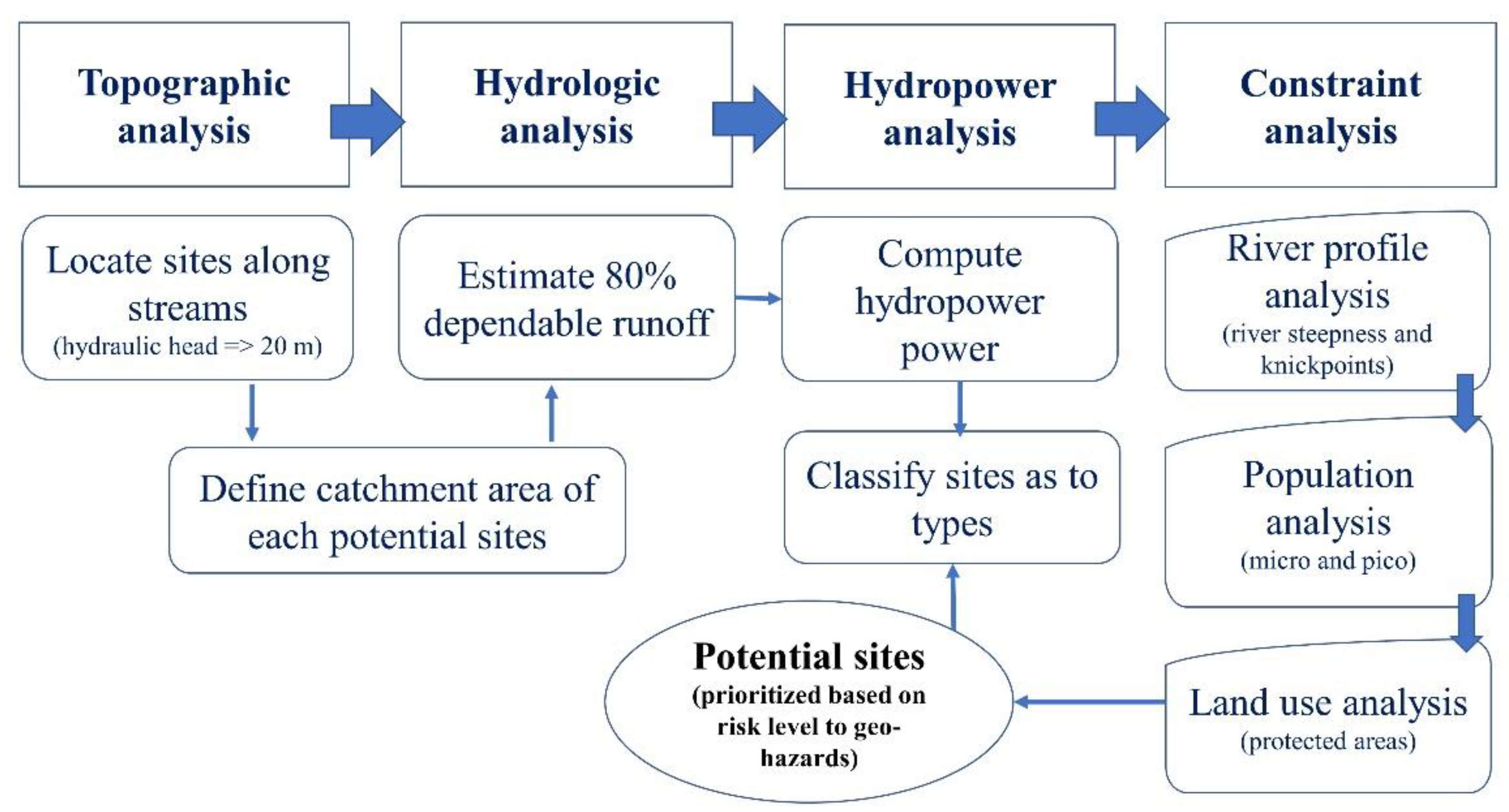
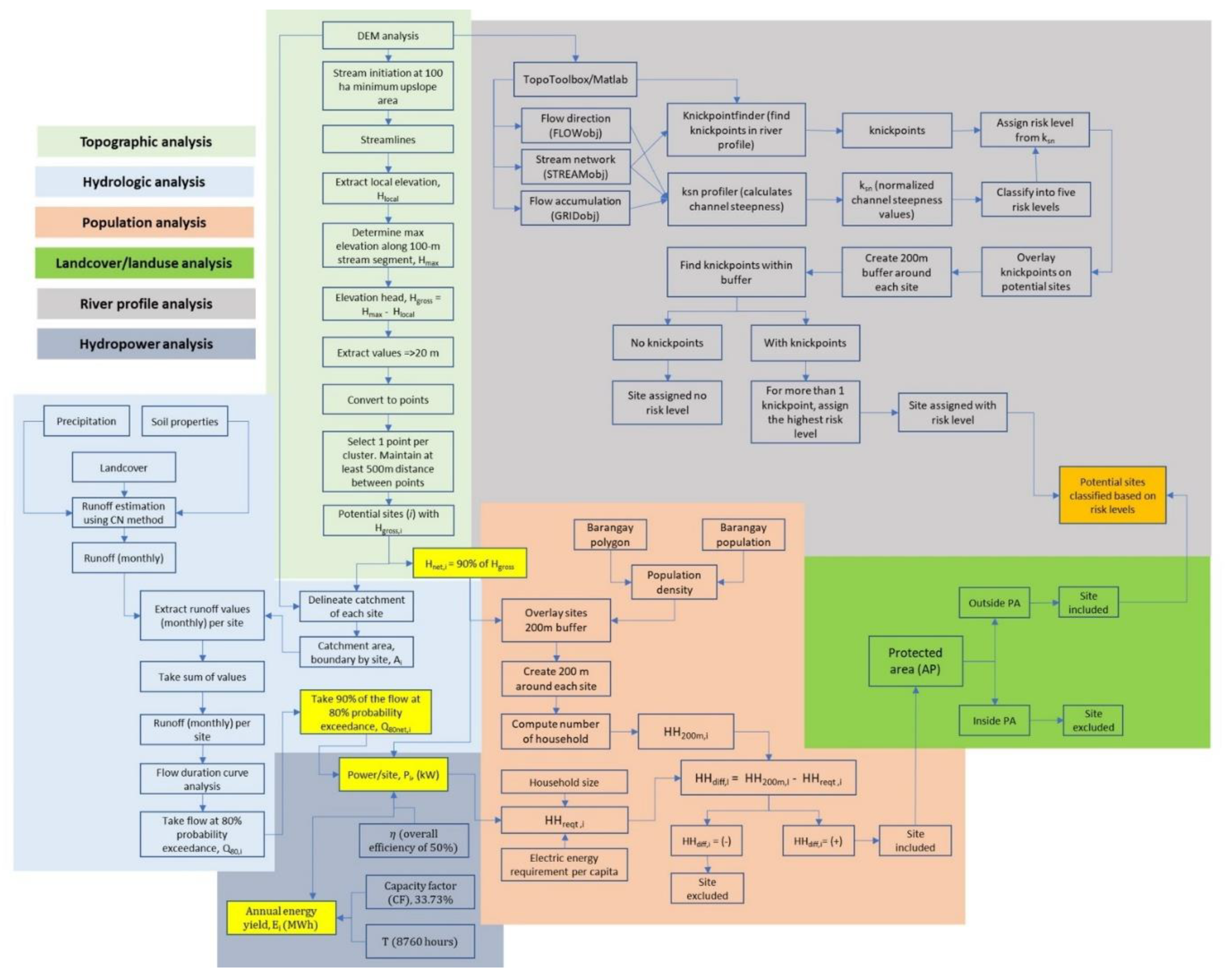
2. Methods
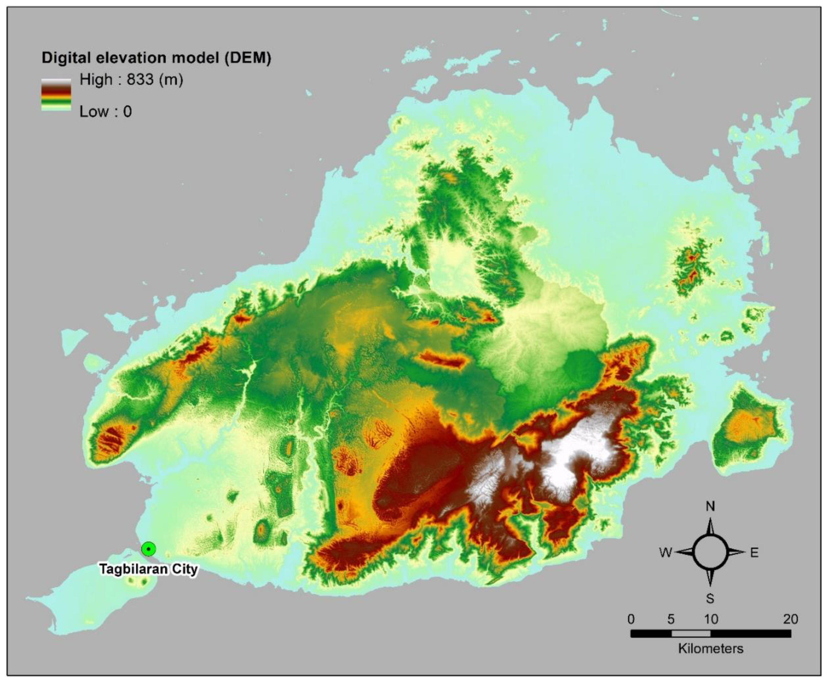
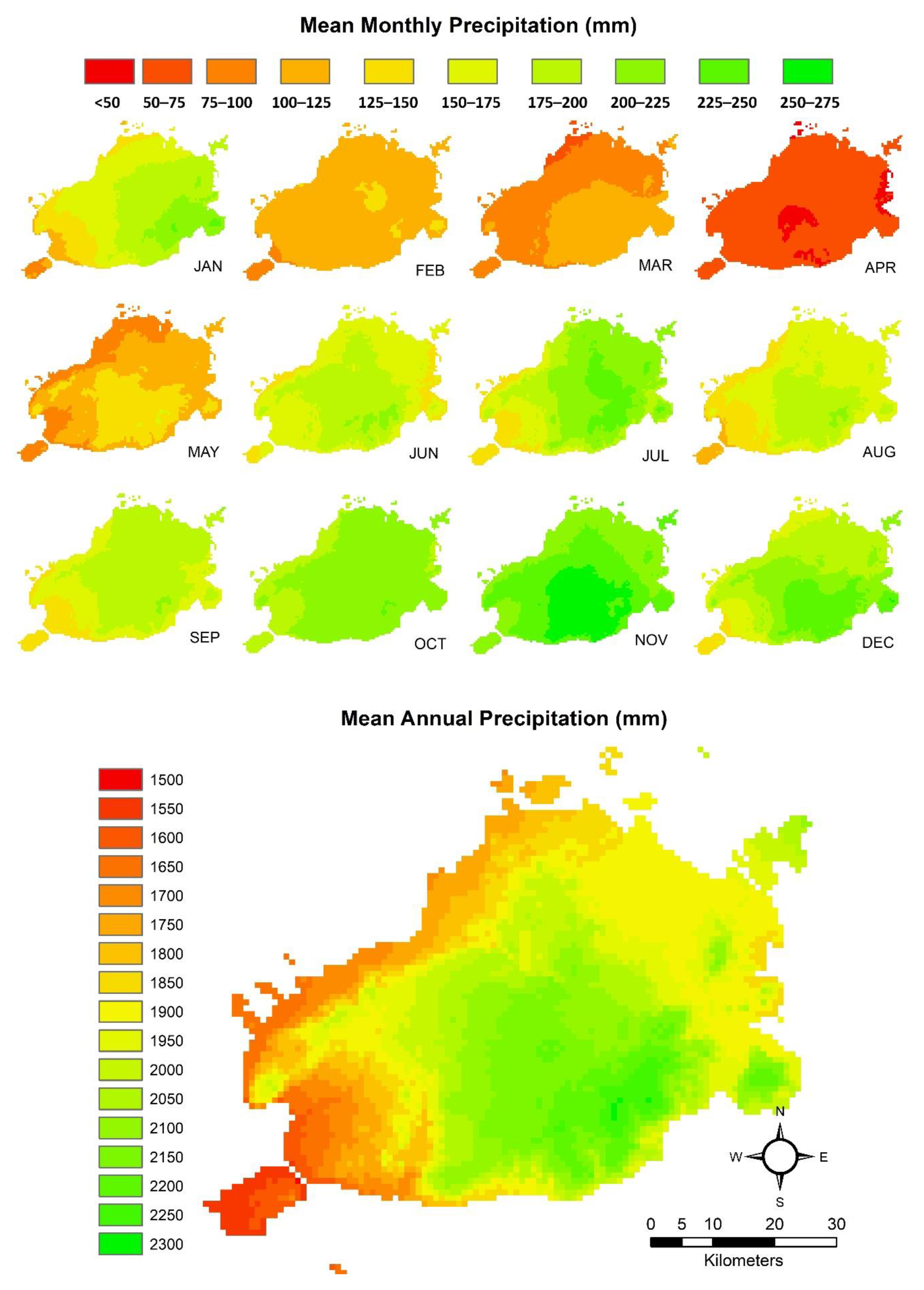
2.1. Datasets
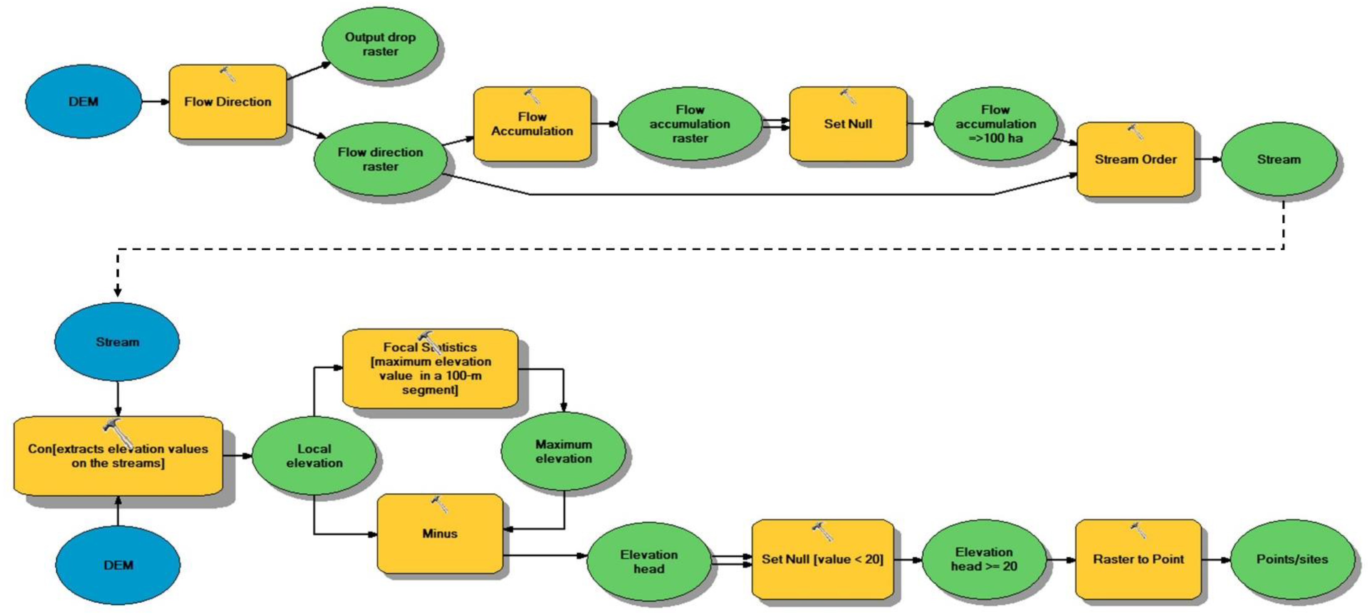
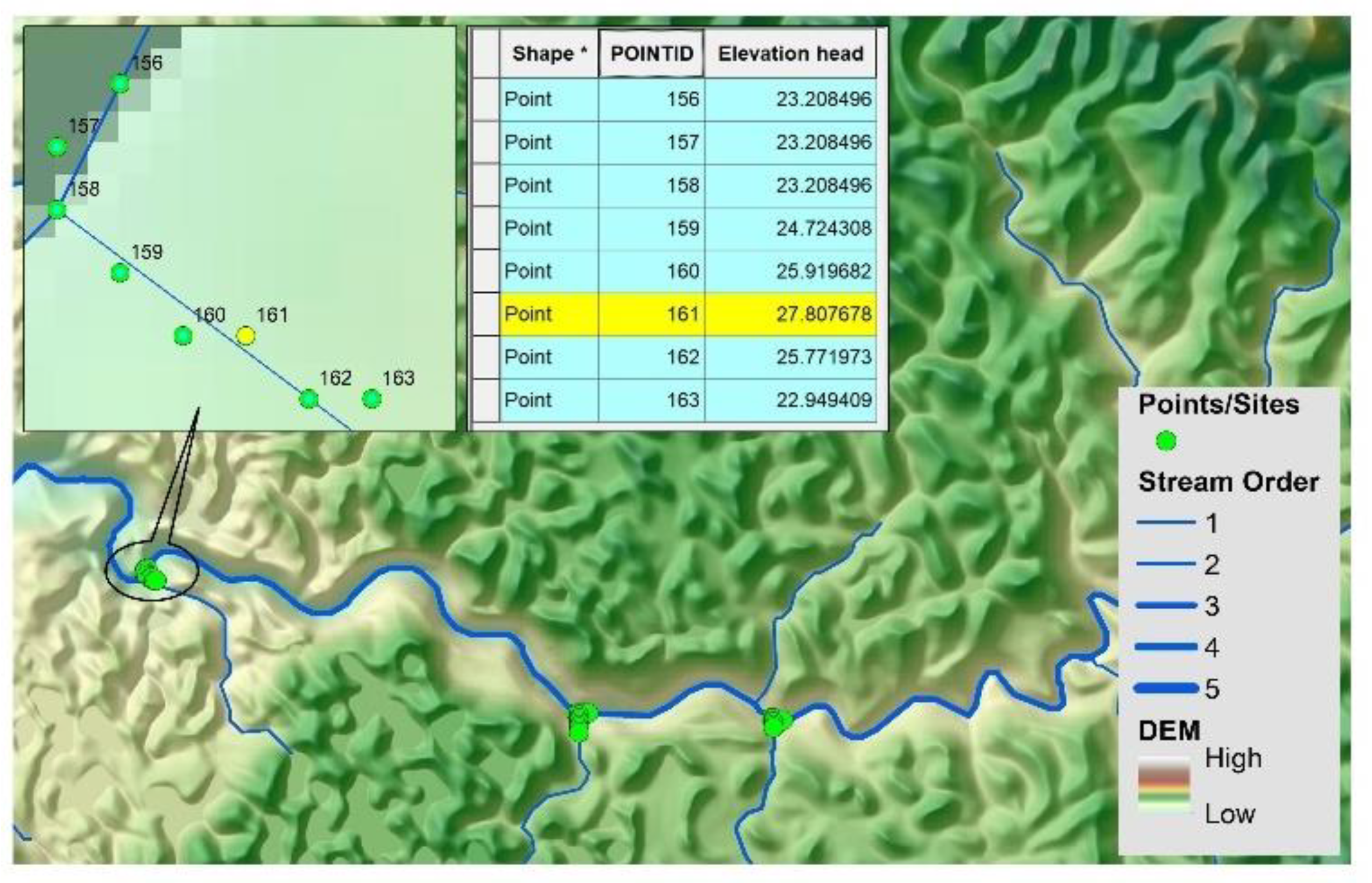
2.2. Topographic Analysis
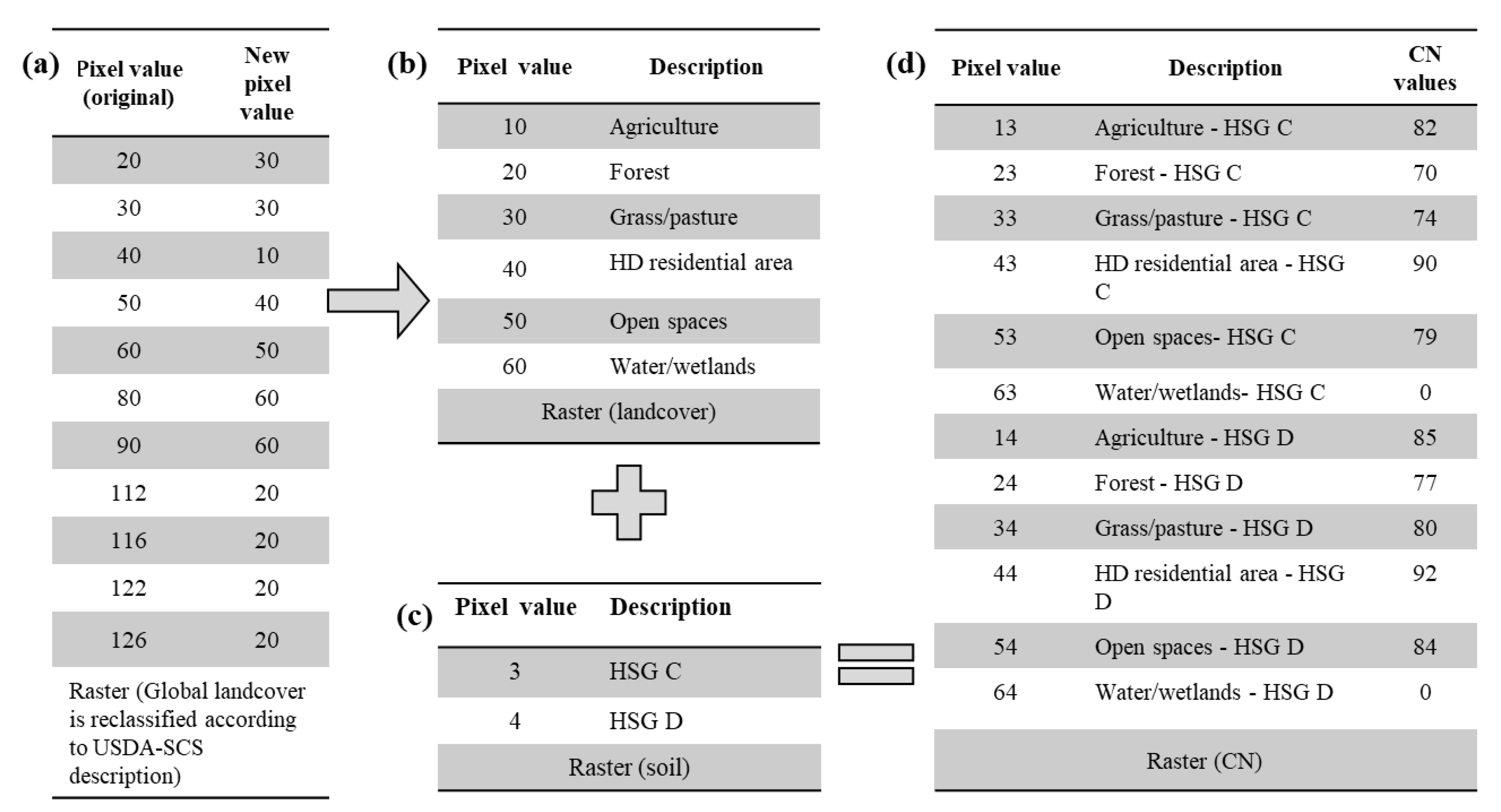
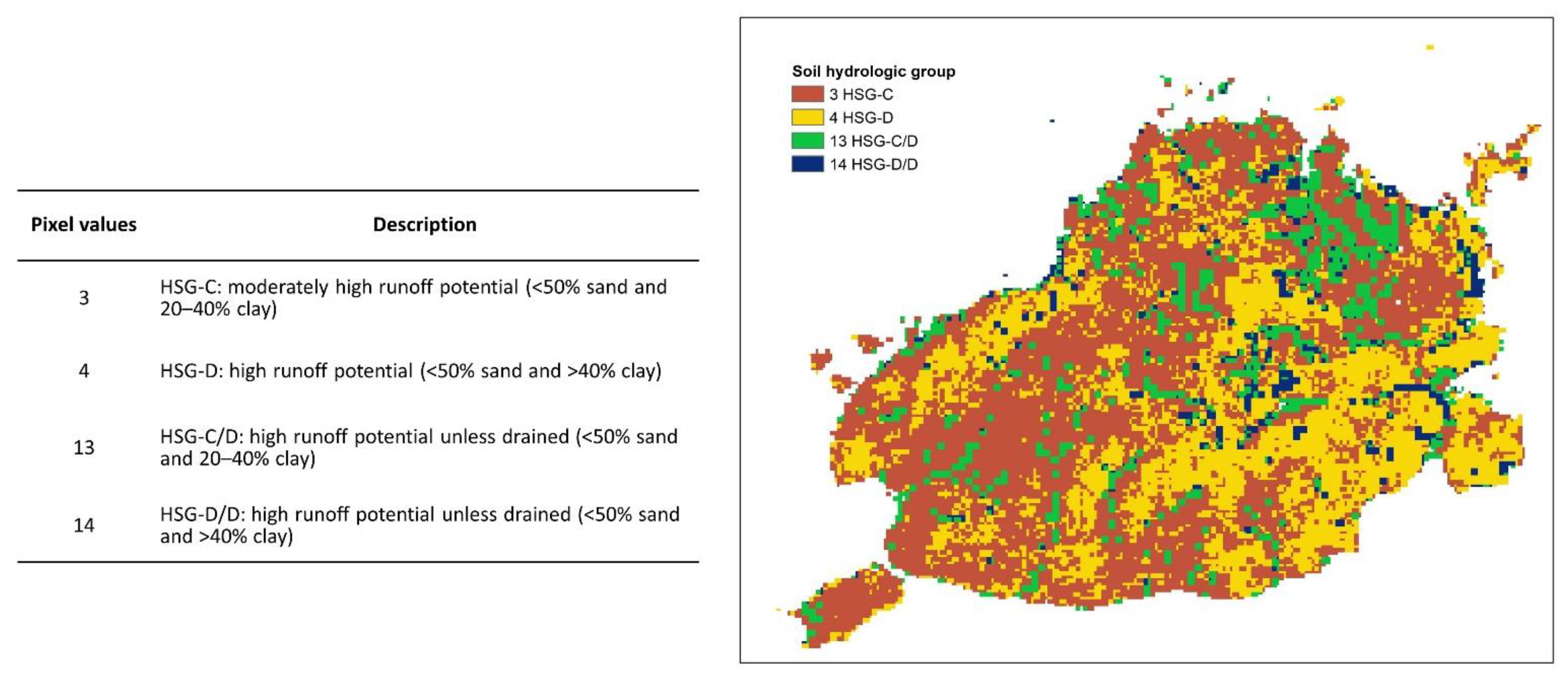
2.3. Runoff Estimation Using CN Method
2.4. Hydropower Capacity and Annual Energy Generation
2.5. River Profile Analysis
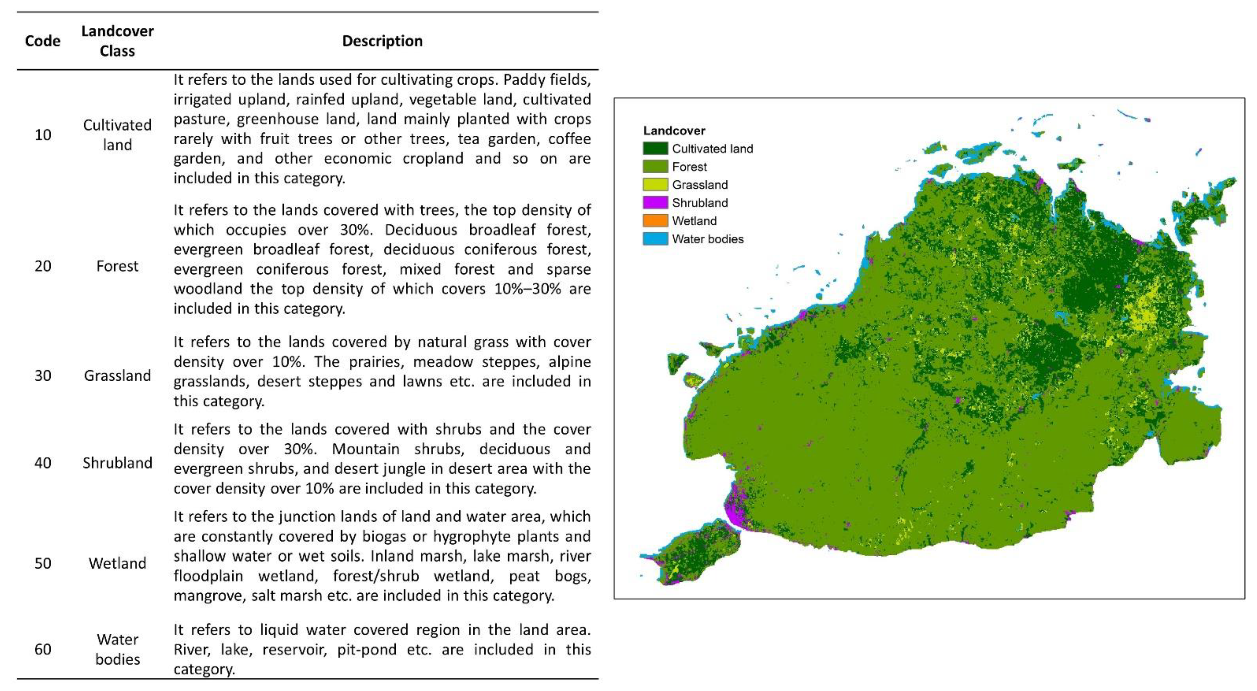
2.6. Land Use and Population Analysis
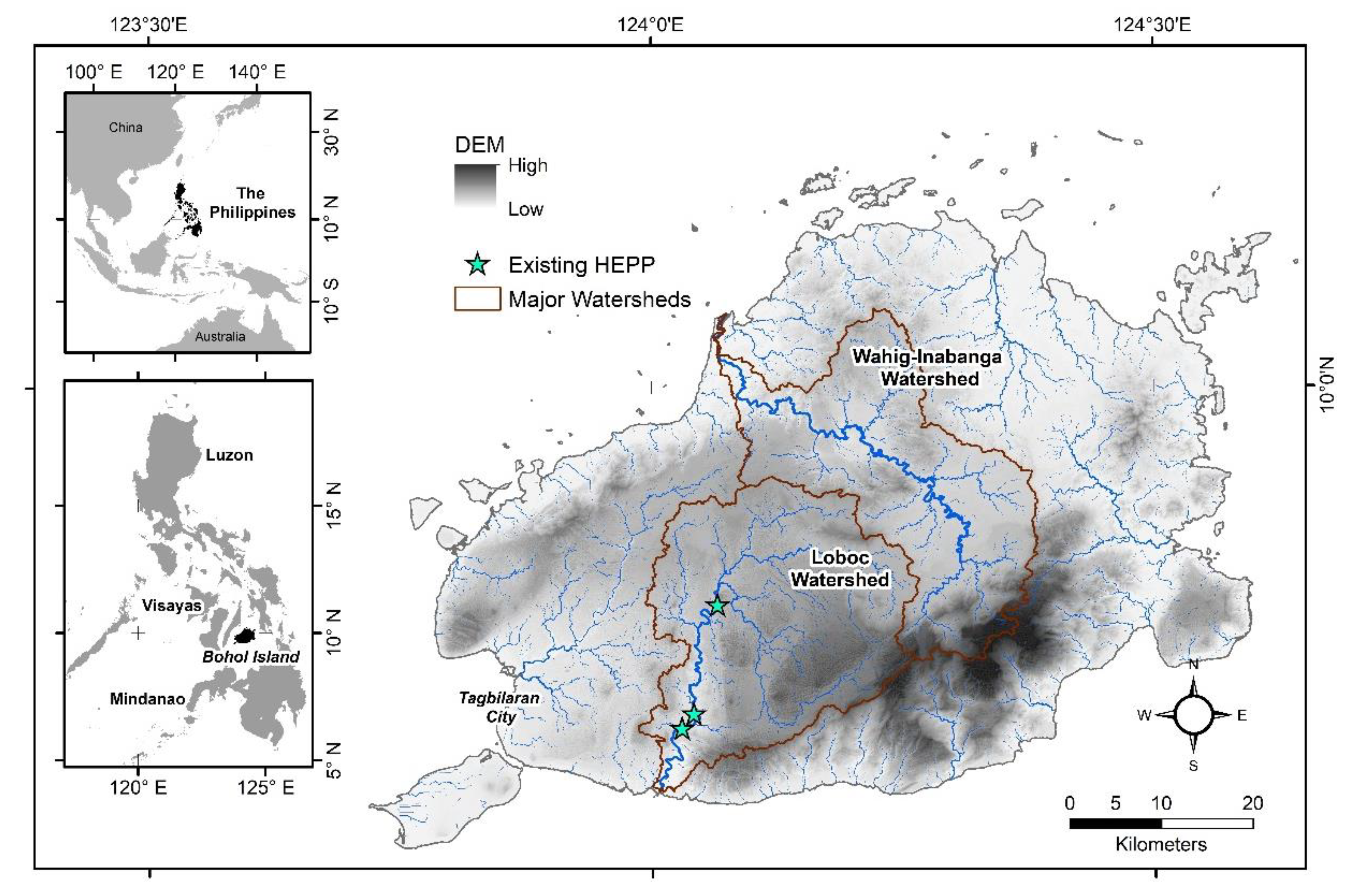
2.7. Case Study Application in Bohol Island, Central Philippines
3. Results
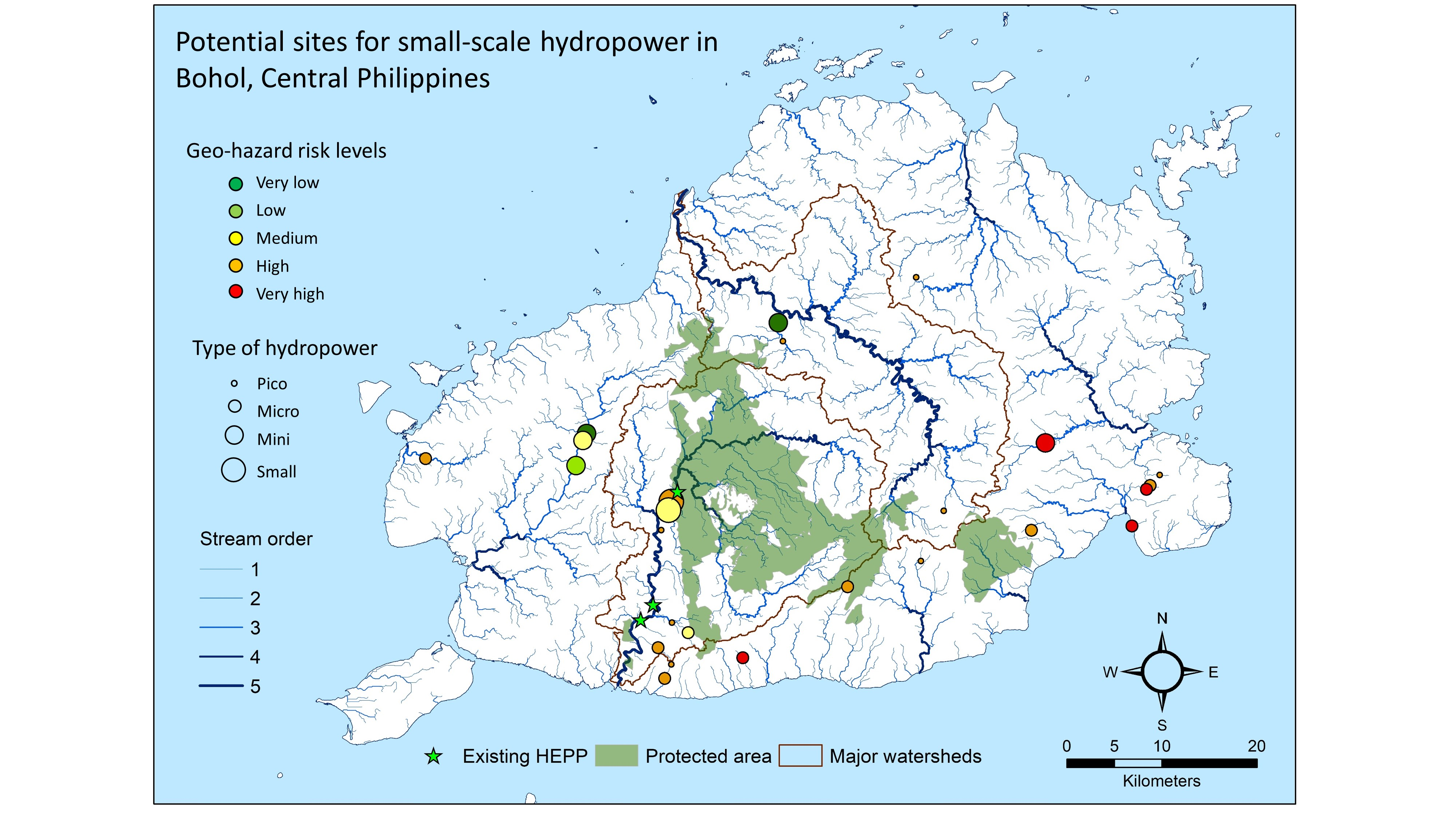
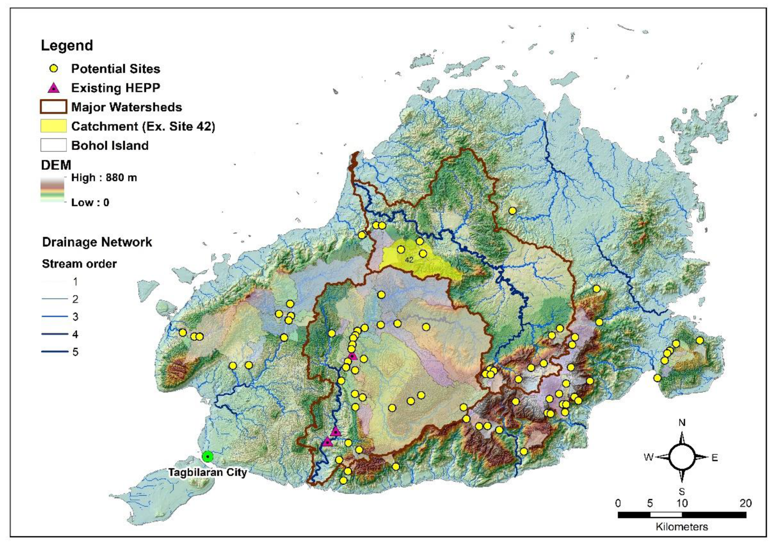
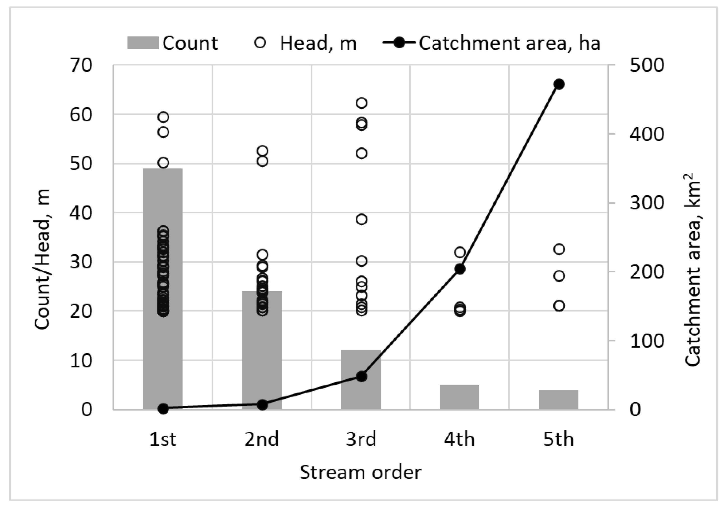
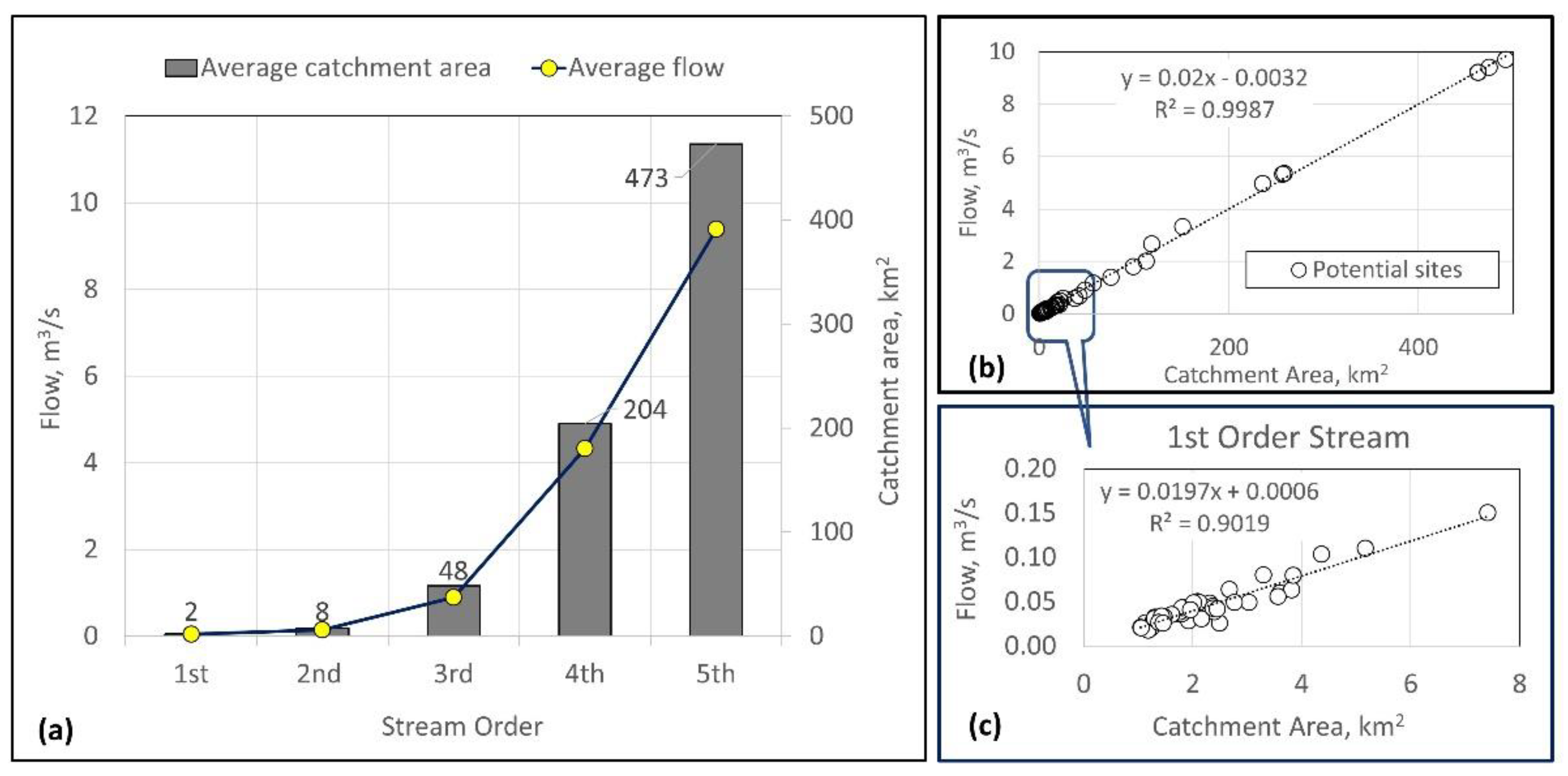
3.1. Landscape-Wide Topographic Analysis and the Potential Sites
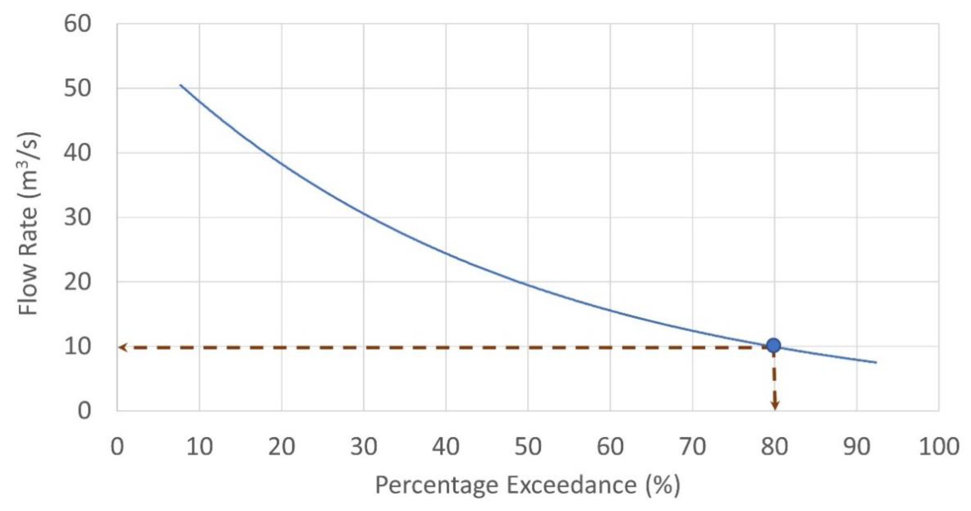
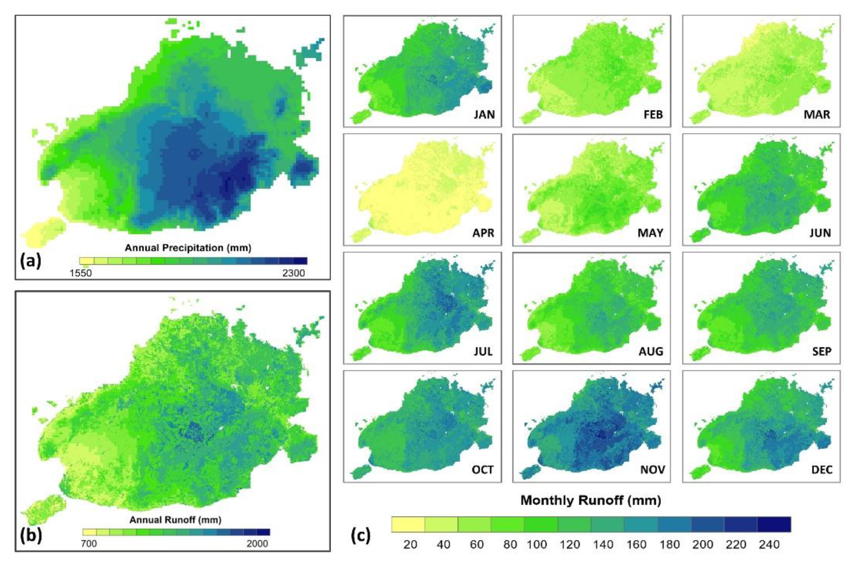
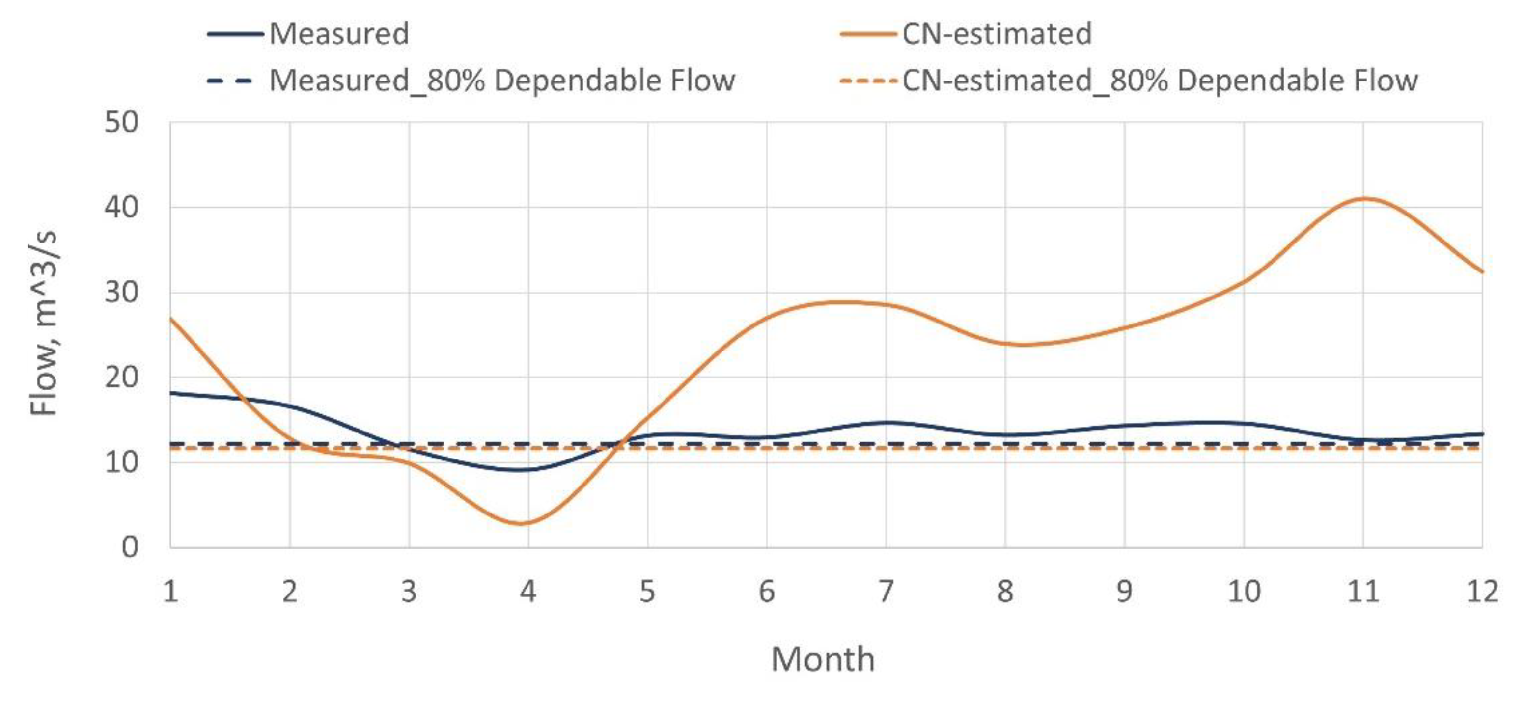
3.2. Runoff Estimates
3.3. Potential Power and Energy Generation
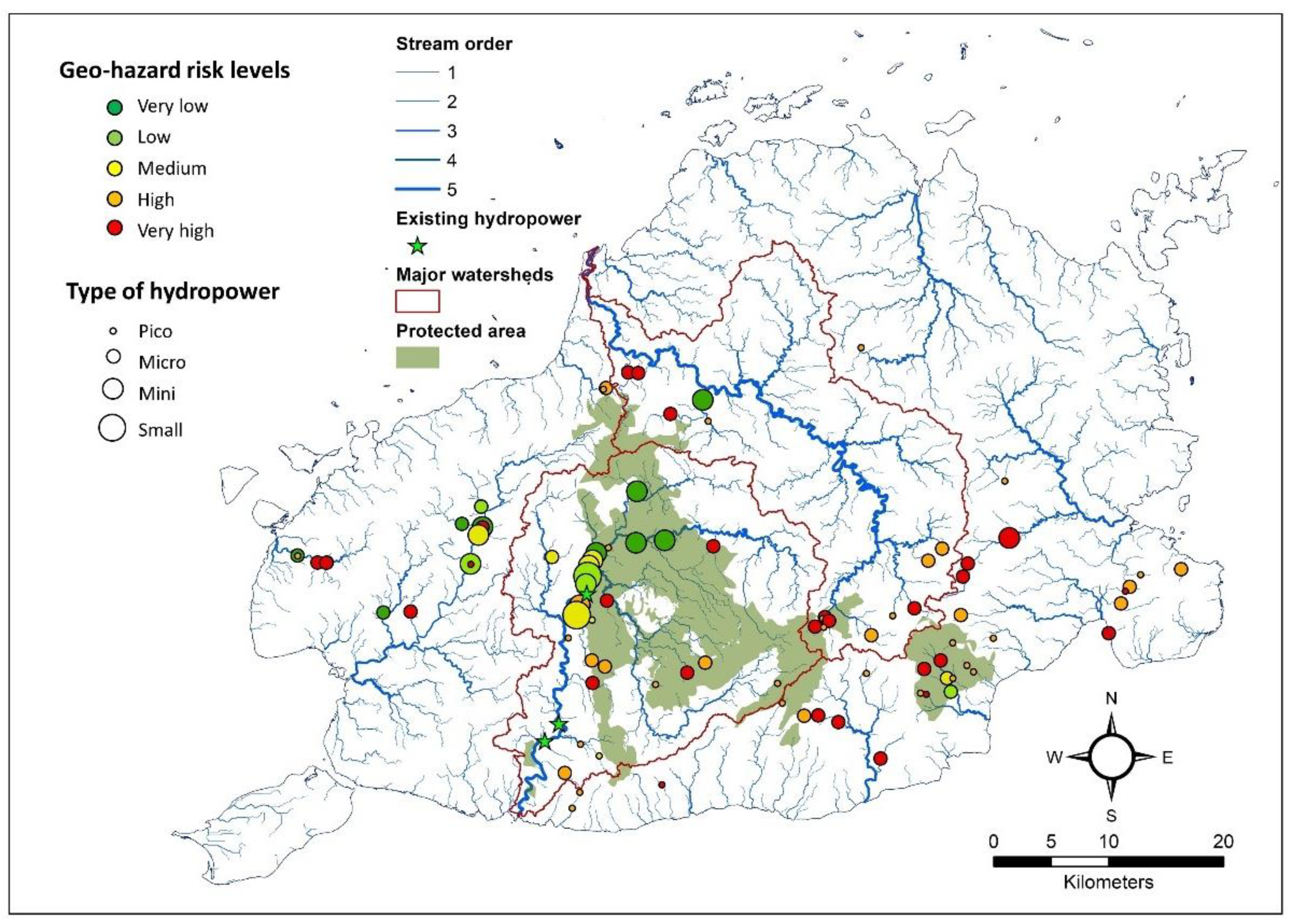
3.4. Geo-Hazard Risks Associated with Each Potential Sites
3.5. Land-Use and Population Constraints
4. Discussion
4.1. Loboc Watershed Hydropower Potential and Environmental Concerns
4.2. Potential Sites Outside of Major Watersheds
4.3. Small-Scale Hydropower Potential in the Island Landscape
4.4. Dataset Limitations
4.5. Geometric Index of Geo-Hazard Risk
4.6. Land-Use Policy and Population Density as Constraints
5. Conclusions
- (a)
- The approach employed in the study reveals potential small-scale hydropower sites inside major and small watersheds. More than half of the identified sites are located outside the major watersheds, with a share of about 21% of the total potential power capacity;
- (b)
- Freely available global datasets are successfully used to estimate runoff using the CN method and found runoff varying spatially and temporally across the landscape and at each potential site;
- (c)
- The hydropower potential in the study area consists of a range of small-scale hydropower systems with different power and energy generation capacities. In terms of number, the micro types dominate in the study area, but four small types provide almost half of the potential hydropower;
- (d)
- Each potential site is found under varying levels of geo-hazard risk innate to the geography and geology of the area. Seventy-four percent (74%) of the sites are under ‘high—very high levels’ of geo-hazard risk, while 52% of the total potential power capacity can be produced from low-risk sites;
- (e)
- The land-use and population analysis found several potential sites inside protected areas and in areas where the number of beneficiaries is still limited. The analysis result reduces the number of sites by 73%, and consequently, power capacity by 60%. Future changes in land-use planning and an increase in population in remote areas are seen to optimize the development of the identified potential sites;
- (f)
- The study produced decision-support maps showing the potential sites’ spatial distribution, the hydropower types and power capacities, and the risk levels associated with each site. The maps are expected to provide crucial information for resource managers and decision-makers.
Author Contributions
Funding
Informed Consent Statement
Data Availability Statement
Acknowledgments
Conflicts of Interest
Appendix A


Appendix B

| Count | Watershed | Catchment ID | Area, ha | Gross Head, m | Flow, m3/s | Power, kW | Annual Energy, kWh | Type | ksn Class | HH200m | HHsite | HHdiff | Protected Area |
|---|---|---|---|---|---|---|---|---|---|---|---|---|---|
| 1 | Other | 1 | 148 | 20.6 | 0.029 | 4 | 11,976 | pico | high | 4.6 | 3.9 | 0.7 | outside |
| 2 | Wahig-Inabanga Watershed | 4 | 1211 | 24.4 | 0.212 | 35 | 103,096 | micro | very high | 2.8 | 33.7 | −30.9 | outside |
| 3 | Wahig-Inabanga Watershed | 13 | 360 | 35.6 | 0.060 | 14 | 42,357 | micro | very high | 8.2 | 13.8 | −5.6 | outside |
| 4 | Other | 19 | 219 | 31.4 | 0.041 | 9 | 25,648 | micro | high | 4.5 | 8.4 | −3.8 | outside |
| 5 | Other | 25 | 250 | 31.0 | 0.026 | 5 | 15,853 | micro | high | 3.8 | 5.2 | −1.3 | outside |
| 6 | Wahig-Inabanga Watershed | 42 | 4867 | 58.4 | 0.902 | 356 | 1,050,624 | mini | very low | 0.0 | 0.0 | 0.0 | outside |
| 7 | Wahig-Inabanga Watershed | 45 | 716 | 26.7 | 0.127 | 23 | 67,614 | micro | very high | 6.3 | 22.1 | −15.8 | outside |
| 8 | Wahig-Inabanga Watershed | 53 | 118 | 32.0 | 0.022 | 5 | 14,033 | pico | high | 6.0 | 4.6 | 1.4 | outside |
| 9 | Other | 60 | 114 | 29.3 | 0.026 | 5 | 15,254 | micro | high | 3.6 | 5.0 | −1.4 | outside |
| 10 | Loboc Watershed | 63 | 748 | 20.8 | 0.135 | 19 | 55,978 | micro | very high | 2.8 | 18.3 | −15.5 | inside |
| 11 | Loboc Watershed | 65 | 5722 | 20.9 | 1.168 | 165 | 488,058 | mini | very low | 0.0 | 0.0 | 0.0 | inside |
| 12 | Other | 68 | 1643 | 24.8 | 0.303 | 51 | 149,926 | micro | very low | 8.6 | 49.0 | −40.4 | outside |
| 13 | Other | 71 | 1759 | 20.2 | 0.322 | 44 | 130,025 | micro | low | 8.6 | 42.5 | −33.9 | outside |
| 14 | Other | 80 | 1303 | 31.6 | 0.232 | 49 | 146,047 | micro | very low | 5.5 | 47.7 | −42.2 | outside |
| 15 | Other | 85 | 7598 | 62.4 | 1.398 | 589 | 1,739,438 | mini | very low | 0.0 | 0.0 | 0.0 | outside |
| 16 | Other | 90 | 382 | 59.6 | 0.063 | 25 | 75,141 | micro | very high | 7.3 | 24.5 | −17.2 | outside |
| 17 | Other | 103 | 356 | 56.5 | 0.056 | 21 | 62,982 | micro | very high | 5.5 | 20.6 | −15.1 | outside |
| 18 | Other | 113 | 9965 | 52.1 | 1.801 | 634 | 1,873,906 | mini | medium | 0.0 | 0.0 | 0.0 | outside |
| 19 | Other | 116 | 2526 | 57.9 | 0.591 | 231 | 682,922 | mini | very high | 0.0 | 0.0 | 0.0 | outside |
| 20 | Loboc Watershed | 125 | 11,876 | 32.1 | 2.661 | 576 | 1,702,843 | mini | very low | 0.0 | 0.0 | 0.0 | inside |
| 21 | Loboc Watershed | 130 | 15,174 | 20.9 | 3.325 | 469 | 1,385,436 | mini | very low | 0.0 | 0.0 | 0.0 | inside |
| 22 | Loboc Watershed | 137 | 994 | 23.8 | 0.203 | 33 | 96,352 | micro | very high | 7.3 | 31.5 | −24.1 | inside |
| 23 | Loboc Watershed | 139 | 124 | 21.0 | 0.021 | 3 | 8644 | pico | high | 3.9 | 2.8 | 1.1 | inside |
| 24 | Wahig-Inabanga Watershed | 141 | 277 | 24.4 | 0.065 | 11 | 31,791 | micro | high | 7.5 | 10.4 | −2.9 | outside |
| 25 | Loboc Watershed | 147 | 1899 | 21.5 | 0.327 | 47 | 140,209 | micro | very high | 4.5 | 45.8 | −41.3 | inside |
| 26 | Loboc Watershed | 150 | 23,594 | 20.4 | 4.967 | 683 | 2,017,384 | mini | very low | 0.0 | 0.0 | 0.0 | inside |
| 27 | Other | 156 | 3787 | 23.2 | 0.587 | 92 | 272,066 | micro | very low | 7.8 | 88.8 | −81.0 | outside |
| 28 | Other | 161 | 192 | 27.8 | 0.028 | 5 | 15,705 | micro | high | 7.8 | 5.1 | 2.7 | outside |
| 29 | Loboc Watershed | 167 | 304 | 29.0 | 0.049 | 10 | 28,505 | micro | medium | 4.3 | 9.3 | −5.0 | outside |
| 30 | Loboc Watershed | 173 | 25,689 | 20.0 | 5.328 | 721 | 2,130,974 | mini | medium | 0.0 | 0.0 | 0.0 | inside |
| 31 | Wahig-Inabanga Watershed | 177 | 209 | 29.1 | 0.050 | 10 | 29,027 | micro | high | 6.3 | 9.5 | −3.2 | outside |
| 32 | Other | 195 | 2147 | 25.0 | 0.344 | 58 | 171,157 | micro | medium | 7.5 | 55.9 | −48.4 | outside |
| 33 | Other | 196 | 240 | 33.0 | 0.039 | 9 | 25,362 | micro | very high | 4.9 | 8.3 | −3.3 | outside |
| 34 | Other | 201 | 841 | 21.9 | 0.124 | 18 | 54,179 | micro | very high | 7.5 | 17.7 | −10.2 | outside |
| 35 | Other | 209 | 767 | 29.3 | 0.179 | 35 | 104,667 | micro | very high | 14.4 | 34.2 | −19.7 | outside |
| 36 | Other | 217 | 11,295 | 30.3 | 2.007 | 411 | 1,214,055 | mini | low | 0.0 | 0.0 | 0.0 | outside |
| 37 | Other | 225 | 216 | 30.3 | 0.031 | 6 | 18,508 | micro | very high | 4.5 | 6.0 | −1.5 | outside |
| 38 | Loboc Watershed | 233 | 25,872 | 20.5 | 5.356 | 740 | 2,186,165 | mini | medium | 0.0 | 0.0 | 0.0 | inside |
| 39 | Other | 234 | 267 | 21.0 | 0.064 | 9 | 26,711 | micro | high | 5.1 | 8.7 | −3.6 | outside |
| 40 | Other | 238 | 175 | 20.0 | 0.036 | 5 | 14,370 | pico | high | 11.1 | 4.7 | 6.4 | outside |
| 41 | Loboc Watershed | 246 | 46,279 | 32.7 | 9.210 | 2031 | 6,001,996 | small | low | 0.0 | 0.0 | 0.0 | inside |
| 42 | Other | 249 | 631 | 21.4 | 0.147 | 21 | 62,926 | micro | very high | 19.3 | 20.5 | −1.3 | outside |
| 43 | Loboc Watershed | 251 | 46,342 | 21.2 | 9.220 | 1322 | 3,905,939 | small | low | 0.0 | 0.0 | 0.0 | inside |
| 44 | Other | 271 | 181 | 32.7 | 0.037 | 8 | 23,857 | micro | high | 9.3 | 7.8 | 1.5 | outside |
| 45 | Other | 284 | 128 | 34.3 | 0.028 | 7 | 19,427 | micro | very high | 11.0 | 6.3 | 4.6 | outside |
| 46 | Loboc Watershed | 300 | 741 | 29.1 | 0.150 | 29 | 87,155 | micro | very high | 3.3 | 28.5 | −25.2 | inside |
| 47 | Other | 315 | 436 | 25.7 | 0.103 | 18 | 52,956 | micro | high | 9.3 | 17.3 | −8.0 | outside |
| 48 | Loboc Watershed | 319 | 47,491 | 21.1 | 9.407 | 1341 | 3,962,478 | small | high | 0.0 | 0.0 | 0.0 | outside |
| 49 | Wahig-Inabanga Watershed | 333 | 394 | 52.7 | 0.091 | 32 | 95,171 | micro | very high | 9.6 | 31.1 | −21.5 | outside |
| 50 | Other | 346 | 718 | 25.2 | 0.090 | 15 | 45,323 | micro | very high | 9.2 | 14.8 | −5.6 | outside |
| 51 | Other | 348 | 4231 | 20.3 | 0.677 | 93 | 273,575 | micro | very low | 9.3 | 89.3 | −80.0 | outside |
| 52 | Loboc Watershed | 357 | 1399 | 50.6 | 0.250 | 86 | 252,673 | micro | very high | 5.6 | 82.5 | −76.9 | outside |
| 53 | Other | 364 | 182 | 27.4 | 0.043 | 8 | 23,702 | micro | high | 7.5 | 7.7 | −0.3 | outside |
| 54 | Loboc Watershed | 365 | 49,226 | 27.3 | 9.709 | 1790 | 5,288,296 | small | medium | 0.0 | 0.0 | 0.0 | outside |
| 55 | Wahig-Inabanga Watershed | 380 | 105 | 27.2 | 0.021 | 4 | 11,416 | pico | high | 4.7 | 3.7 | 1.0 | outside |
| 56 | Wahig-Inabanga Watershed | 403 | 517 | 36.4 | 0.110 | 27 | 79,789 | micro | very high | 7.0 | 26.1 | −19.0 | inside |
| 57 | Wahig-Inabanga Watershed | 409 | 177 | 20.3 | 0.039 | 5 | 15,693 | micro | high | 6.2 | 5.1 | 1.0 | inside |
| 58 | Loboc Watershed | 418 | 214 | 22.3 | 0.039 | 6 | 17,460 | micro | medium | 2.6 | 5.7 | −3.1 | inside |
| 59 | Wahig-Inabanga Watershed | 430 | 508 | 29.0 | 0.109 | 21 | 63,166 | micro | very high | 5.8 | 20.6 | −14.9 | inside |
| 60 | Wahig-Inabanga Watershed | 446 | 142 | 50.3 | 0.032 | 11 | 31,997 | micro | very high | 3.7 | 10.4 | −6.8 | inside |
| 61 | Wahig-Inabanga Watershed | 457 | 138 | 23.9 | 0.030 | 5 | 14,222 | pico | high | 2.3 | 4.6 | −2.4 | outside |
| 62 | Other | 462 | 231 | 28.2 | 0.049 | 9 | 27,272 | micro | very high | 14.9 | 8.9 | 6.0 | outside |
| 63 | Wahig-Inabanga Watershed | 468 | 384 | 20.1 | 0.080 | 11 | 31,940 | micro | high | 3.5 | 10.4 | −7.0 | outside |
| 64 | Loboc Watershed | 471 | 118 | 25.5 | 0.018 | 3 | 8996 | pico | high | 8.1 | 2.9 | 5.2 | outside |
| 65 | Other | 475 | 180 | 26.0 | 0.043 | 8 | 22,328 | micro | high | 8.6 | 7.3 | 1.3 | outside |
| 66 | Other | 480 | 130 | 22.7 | 0.032 | 5 | 14,689 | pico | high | 9.2 | 4.8 | 4.4 | inside |
| 67 | Loboc Watershed | 482 | 425 | 22.0 | 0.081 | 12 | 35,507 | micro | high | 5.9 | 11.6 | −5.7 | inside |
| 68 | Other | 483 | 330 | 21.2 | 0.080 | 11 | 33,869 | micro | very high | 6.8 | 11.1 | −4.3 | inside |
| 69 | Loboc Watershed | 489 | 237 | 25.7 | 0.045 | 8 | 22,968 | micro | high | 3.3 | 7.5 | −4.2 | inside |
| 70 | Other | 492 | 133 | 21.4 | 0.031 | 5 | 13,332 | pico | high | 13.0 | 4.4 | 8.6 | inside |
| 71 | Loboc Watershed | 493 | 306 | 20.3 | 0.060 | 8 | 24,216 | micro | high | 6.0 | 7.9 | −1.9 | inside |
| 72 | Other | 497 | 161 | 36.3 | 0.035 | 9 | 25,632 | micro | very high | 5.7 | 8.4 | −2.6 | inside |
| 73 | Other | 510 | 212 | 20.1 | 0.049 | 7 | 19,777 | micro | high | 10.9 | 6.5 | 4.5 | inside |
| 74 | Loboc Watershed | 517 | 274 | 26.3 | 0.055 | 10 | 29,070 | micro | very high | 4.1 | 9.5 | −5.4 | inside |
| 75 | Other | 522 | 134 | 20.0 | 0.030 | 4 | 11,794 | pico | high | 5.0 | 3.9 | 1.1 | outside |
| 76 | Other | 527 | 1931 | 38.8 | 0.434 | 114 | 335,958 | mini | medium | 0.0 | 0.0 | 0.0 | inside |
| 77 | Other | 530 | 202 | 21.6 | 0.049 | 7 | 21,022 | micro | high | 9.1 | 6.9 | 2.3 | inside |
| 78 | Loboc Watershed | 536 | 765 | 26.1 | 0.146 | 26 | 76,253 | micro | very high | 4.7 | 24.9 | −20.2 | inside |
| 79 | Loboc Watershed | 546 | 148 | 20.3 | 0.033 | 5 | 13,350 | pico | high | 5.9 | 4.4 | 1.5 | inside |
| 80 | Loboc Watershed | 549 | 141 | 35.2 | 0.030 | 7 | 20,722 | micro | high | 39.6 | 6.8 | 32.9 | inside |
| 81 | Other | 557 | 2201 | 26.2 | 0.494 | 87 | 258,118 | micro | low | 12.8 | 84.3 | −71.4 | inside |
| 82 | Other | 562 | 130 | 27.7 | 0.031 | 6 | 17,264 | micro | high | 7.9 | 5.6 | 2.3 | inside |
| 83 | Other | 567 | 143 | 25.0 | 0.034 | 6 | 16,776 | micro | very high | 8.9 | 5.5 | 3.4 | inside |
| 84 | Other | 576 | 138 | 33.1 | 0.027 | 6 | 17,661 | micro | high | 6.0 | 5.8 | 0.3 | outside |
| 85 | Other | 582 | 502 | 24.2 | 0.097 | 16 | 46,588 | micro | very high | 4.7 | 15.2 | −10.5 | outside |
| 86 | Other | 588 | 293 | 21.9 | 0.055 | 8 | 24,201 | micro | high | 5.8 | 7.9 | −2.1 | outside |
| 87 | Other | 589 | 958 | 20.9 | 0.186 | 26 | 77,659 | micro | very high | 4.2 | 25.4 | −21.2 | outside |
| 88 | Loboc Watershed | 592 | 146 | 21.9 | 0.026 | 4 | 11,349 | pico | high | 7.9 | 3.7 | 4.2 | outside |
| 89 | Loboc Watershed | 595 | 196 | 22.2 | 0.041 | 6 | 18,114 | micro | medium | 6.6 | 5.9 | 0.7 | outside |
| 90 | Other | 598 | 555 | 23.8 | 0.128 | 21 | 60,815 | micro | very high | 8.8 | 19.9 | −11.1 | outside |
| 91 | Loboc Watershed | 602 | 237 | 33.5 | 0.043 | 10 | 28,374 | micro | high | 25.8 | 9.3 | 16.5 | outside |
| 92 | Other | 608 | 245 | 23.5 | 0.042 | 7 | 19,643 | micro | very high | 7.8 | 6.4 | 1.4 | outside |
| 93 | Other | 616 | 106 | 22.3 | 0.020 | 3 | 9042 | pico | high | 13.2 | 3.0 | 10.3 | outside |
| 94 | Other | 618 | 277 | 20.3 | 0.049 | 7 | 19,875 | micro | high | 17.8 | 6.5 | 11.3 | outside |
References
- Avtar, R.; Sahu, N.; Aggarwal, A.K.; Chakraborty, S.; Kharrazi, A.; Yunus, A.P.; Dou, J.; Kurniawan, T.A. Exploring Renewable Energy Resources Using Remote Sensing and GIS—A Review. Resources 2019, 8, 149. [Google Scholar] [CrossRef]
- Hoes, O.A.C.; Meijer, L.J.J.; van der Ent, R.J.; van De, N.C. Systematic high-resolution assessment of global hydropower potential. PLoS ONE 2017, 12, e0171844. [Google Scholar] [CrossRef]
- JICA. Guideline and Manual for Hydropower Development Vol 2 Small Scale Hydropower. 2011. Available online: https://openjicareport.jica.go.jp/pdf/12024899.pdf (accessed on 3 July 2020).
- Province of Bohol. Bohol Island Power Development Plan (BIPDP). 2017. Available online: http://www.ppdobohol.lgu.ph/plan-reports/development-plans/bohol-island-power-development-plan-bipdp/ (accessed on 21 May 2020).
- Yi, C.S.; Lee, J.H.; Shim, M.P. Site location analysis for small hydropower using geo-spatial information system. Renew. Energy 2010, 35, 852–861. [Google Scholar] [CrossRef]
- Zhang, J.; Xu, L.; Li, X. Review on the externalities of hydropower: A comparison between large and small hydropower projects in Tibet based on the CO2 equivalent. Renew. Sustain. Energy Rev. 2015, 50, 176–185. [Google Scholar] [CrossRef]
- IRENA. Renewables Readiness Assessment: The Philippines. Int. Renew. Energy Agency 2017, 10, 79–89. Available online: https://www.irena.org/publications/2017/Mar/Renewables-Readiness-Assessment-The-Philippines (accessed on 20 June 2021).
- Faruqui, N.I. Small hydro for rural development. Can. Water Resour. J. 1994, 19, 227–235. [Google Scholar] [CrossRef][Green Version]
- Mayor, B.; Rodríguez-Muñoz, I.; Villarroya, F.; Montero, E.; López-Gunn, E. The role of large and small scale hydropower for energy and water security in the Spanish Duero basin. Sustainability 2017, 9, 1807. [Google Scholar] [CrossRef]
- Asian Development Bank. The Philippines: Energy Sector Assessment, Strategy, and Road Map. 2016. Available online: https://www.adb.org/sites/default/files/institutional-document/218286/mya-energy-sector-assessment.pdf (accessed on 5 May 2020).
- Philippine Department of Energy. Renewable Energy Decade Report 2008–2018. 2019. Available online: https://www.doe.gov.ph/renewable-energy/empowered-renewable-energy-decade-report-2008-2018?ckattempt=1 (accessed on 12 January 2021).
- Fasipe, O.A.; Izinyon, O.C.; Ehiorobo, J.O. Hydropower potential assessment using spatial technology and hydrological modelling in Nigeria river basin. Renew. Energy 2021, 178, 960–976. [Google Scholar] [CrossRef]
- Moiz, A.; Kawasaki, A.; Koike, T.; Shrestha, M. A systematic decision support tool for robust hydropower site selection in poorly gauged basins. Appl. Energy 2018, 224, 309–321. [Google Scholar] [CrossRef]
- Thin, K.K.; Zin, W.W.; San, Z.M.L.T.; Kawasaki, A.; Moiz, A.; Bhagabati, S.S. Estimation of run-of-river hydropower potential in the myitnge river basin. J. Disaster Res. 2020, 15, 267–276. [Google Scholar] [CrossRef]
- Bayazıt, Y.; Bakış, R.; Koç, C. An investigation of small scale hydropower plants using the geographic information system. Renew. Sustain. Energy Rev. 2017, 67, 289–294. [Google Scholar] [CrossRef]
- Sammartano, V.; Liuzzo, L.; Freni, G. Identification of potential locations for run-of-river hydropower plants using a GIS-based procedure. Energies 2019, 12, 3446. [Google Scholar] [CrossRef]
- Tarife, R.P.; Tahud, A.P.; Gulben, E.J.G.; Macalisang, H.A.R.C.P.; Ignacio, M.T.T. Application of geographic information system (GIS) in hydropower resource assessment: A case study in Misamis Occidental, Philippines. Int. J. Environ. Sci. Dev. 2017, 8, 507–511. [Google Scholar] [CrossRef]
- Guiamel, I.A.; Lee, H.S. Potential hydropower estimation for the Mindanao River Basin in the Philippines based on watershed modelling using the soil and water assessment tool. Energy Rep. 2020, 6, 1010–1028. [Google Scholar] [CrossRef]
- Jafari, M.; Fazloula, R.; Effati, M.; Jamali, A. Providing a GIS-based framework for Run-Of-River hydropower site selection: A model based on sustainable development energy approach. Civ. Eng. Environ. Syst. 2021, 38, 102–126. [Google Scholar] [CrossRef]
- Tamm, O.; Tamm, T. Verification of a robust method for sizing and siting the small hydropower run-of-river plant potential by using GIS. Renew. Energy 2020, 155, 153–159. [Google Scholar] [CrossRef]
- Marston, R.A.; Butler, W.D.; Patch, N.L. Geomorphic Hazards. In International Encyclopedia of Geography: People, the Earth, Environment and Technology; John Wiley & Sons, Inc.: Hoboken, NJ, USA, 2017. [Google Scholar]
- Schwanghart, W.; Ryan, M.; Korup, O. Topographic and seismic constraints on the vulnerability of Himalayan hydropower. Geophys. Res. Lett. 2018, 45, 8985–8992. [Google Scholar] [CrossRef]
- Geach, M.R.; Stokes, M.; Hart, A. The application of geomorphic indices in terrain analysis for ground engineering practice. Eng. Geol. 2017, 217, 122–140. [Google Scholar] [CrossRef]
- Mudd, S.M.; Clubb, F.J.; Gailleton, B.; Hurst, M.D. How concave are river channels? Earth Surf. Dyn. 2018, 6, 505–523. [Google Scholar] [CrossRef]
- Whipple, K.X.; Tucker, G.E. Dynamics of the stream-power river incision model: Implications for height limits of mountain ranges, landscape response timescales, and research needs. J. Geophys. Res. 1999, 104, 661–674. [Google Scholar] [CrossRef]
- Boulton, S.J. Geomorphic response to differential uplift: River long profiles and knickpoints from Guadalcanal and Makira (Solomon Islands). Front. Earth Sci. 2020, 8, 1–23. [Google Scholar] [CrossRef]
- Castillo, M.; Muñoz-Salinas, E.; Ferrari, L. Response of a landscape to tectonics using channel steepness indices (ksn) and OSL: A case of study from the Jalisco Block, Western Mexico. Geomorphology 2014, 221, 204–214. [Google Scholar] [CrossRef]
- Schwanghart, W.; Scherler, D. Short Communication: TopoToolbox 2-MATLAB-based software for topographic analysis and modeling in Earth surface sciences. Earth Surf. Dyn. 2014, 2, 1–7. [Google Scholar] [CrossRef]
- Chen, Y.W.; Shyu, J.B.H.; Chang, C.P. Neotectonic characteristics along the eastern flank of the Central Range in the active Taiwan orogen inferred from fluvial channel morphology. Tectonics 2015, 34, 2249–2270. [Google Scholar] [CrossRef]
- Ross, C.W.; Prihodko, J.Y.L.; Anchang, S.S.K.; Ji, W.; Hanan, N.P. Global Hydrologic Soil Groups (HYSOGs250m) for Curve Number-Based Runoff Modeling. Sci. Data 2018, 5, 180091. [Google Scholar] [CrossRef] [PubMed]
- Buchhorn, M.; Smets, B.; Bertels, L.; De Roo, B.; Lesiv, M.; Tsendbazar, N.E.; Li, L.; Tarko, A.J. Copernicus Global Land Service: Land Cover 100m: Version 3 Globe 2015–2019: Product User Manual; Zenodo: Geneve, Switzerland, September 2020; pp. 1–93. [Google Scholar] [CrossRef]
- Fick, S.E.; Hijmans, R.J. WorldClim 2: New 1-km spatial resolution climate surfaces for global land areas. Int. J. Climatol. 2017, 37, 4302–4315. [Google Scholar] [CrossRef]
- Pojadas, D.J.; Abundo, M.L.S. Spatio-temporal assessment and economic analysis of a grid-connected island province toward a 35% or greater domestic renewable energy portfolio: A case in Bohol, Philippines. Int. J. Energy Environ. Eng. 2021, 12, 251–280. [Google Scholar] [CrossRef]
- Bergström, D.; Malmros, C. Finding Potential Sites for Small-Scale Hydro Power in Uganda: A Step to Assist the Rural Electrification by the Use of GIS. Geobiosphere Science Centre, Department 2005, 95. Available online: http://www.natgeo.lu.se/ex-jobb/exj_121.pdf (accessed on 14 April 2020).
- Arthur, E.; Anyemedu, F.O.K.; Gyamfi, C.; Tannor, P.A.; Adjei, K.A.; Anornu, G.K.; Odai, S.N. Potential for small hydropower development in the Lower Pra River Basin, Ghana. J. Hydrol. Reg. Stud. 2020, 32, 100757. [Google Scholar] [CrossRef]
- Sekac, T.; Jana, S.K.; Pal, D.K. Identifying potential sites for hydropower plant development in Busu catchment: Papua New Guinea. Spat. Inf. Res. 2017, 25, 791–800. [Google Scholar] [CrossRef]
- Tian, Y.; Zhang, F.; Yuan, Z.; Che, Z.; Zafetti, N. Assessment power generation potential of small hydropower plants using GIS software. Energy Rep. 2020, 6, 1393–1404. [Google Scholar] [CrossRef]
- Hashim, H.Q.; Sayl, K.N. Detection of suitable sites for rainwater harvesting planning in an arid region using geographic information system. Appl. Geomat. 2020, 13, 235–248. [Google Scholar] [CrossRef]
- USDA-NRCS. Part 630 Hydrology National Engineering Handbook Chapter 7 Hydrologic Soil Groups. In National Engineering Handbook; Natural Resources Conservation Services—United States Department of Agriculture: Washington DC, USA, 2009. [Google Scholar]
- NWRB-DENR. Resolution No. 03 0613. Revised Policy on Granting Water Rights over Surface Water or Hydropwer Projects. 2013. Available online: http://www.nwrb.gov.ph/images/Board_Resolution/Res_03-0613.pdf (accessed on 14 May 2021).
- Singh, D. Micro Hydro Power Resource Assessment Handbook; Asian and Pacific Centre for Transfer of Technology of the United Nations—Economic and Social Commission for Asia and the Pacific (ESCAP): New Delhi, India, 2009; p. 69. [Google Scholar]
- Mdee, O.J.; Kimambo, C.Z.; Nielsen, T.K.; Kihedu, J. Measurement methods for hydropower resources: A review. Water Util. J. 2018, 18, 21–38. [Google Scholar]
- Wobus, C.; Whipple, K.X.; Kirby, E.; Snyder, N.; Johnson, J.; Spyropolou, K.; Crosby, B.; Sheehan, D. Tectonics from topography: Procedures, promise, and pitfalls. Tecton. Clim. Landsc. E 2006, 398, 55–74. [Google Scholar] [CrossRef]
- Kothyari, G.C.; Kotlia, B.S.; Talukdar, R.; Pant, C.C.; Joshi, M. Evidences of neotectonic activity along Goriganga River, Higher Central Kumaun Himalaya, India. Geol. J. 2020, 55, 6123–6146. [Google Scholar] [CrossRef]
- Lague, D. The stream power river incision model: Evidence, theory and beyond. Earth Surf. Process. Landf. 2014, 39, 38–61. [Google Scholar] [CrossRef]
- Willett, S.D.; McCoy, S.W.; Perron, J.T.; Goren, L.; Chen, C.Y. Dynamic reorganization of River Basins. Science 2014, 343, 1–19. [Google Scholar] [CrossRef]
- Harel, M.A.; Mudd, S.M.; Attal, M. Global analysis of the stream power law parameters based on worldwide 10Be denudation rates. Geomorphology 2016, 268, 184–196. [Google Scholar] [CrossRef]
- Kirby, E.; Whipple, K.X. Expression of active tectonics in erosional landscapes. J. Struct. Geol. 2012, 44, 54–75. [Google Scholar] [CrossRef]
- UNEP-WCMC. User Manual for the World Database on Protected Areas and World Database on Other Effective Area-Based Conservation Measures: 1.6; NEP-WCMC: Cambridge, UK, 2019; Available online: http://wcmc.io/WDPA_manual (accessed on 4 April 2020).
- RA No. 11038. Expanded National Integrated Protected Areas Sytem (NIPAS) Act of 2018; Congress of the Philippines: Manila, Philippines, 2018.
- Philippine Statistics Authority. Highlights on Household Population, Number of Households, and Average Household Size of the Philippines (2015 Census of Population). 2016. Available online: https://psa.gov.ph/content/highlights-household-population-number-households-and-average-household-size-philippines#:~:text=Thecountry’saveragehouseholdsize,to4.4personsin2015 (accessed on 8 June 2021).
- Philippine Department of Energy. List of Existing Power Plants (Grid-Connected) As of June 2019 Department of Energy List of Existing Power Plants (Grid-Connected) As of June 2019; Philippine Department of Energy: Manila, Philippines, 2019.
- Carrasco, J.L.; Pain, A.; Spuhler, D. Hydropower (Small-Scale). Sustainable Sanitation and Water Management Toolbox-SSWM.info. 2019. Available online: https://sswm.info/water-nutrient-cycle/water-distribution/hardwares/water-network-distribution/hydropower-%28small-scale%29 (accessed on 2 June 2020).
- Tucker, G.E.; Hancock, G.R. Modelling landscape evolution. Earth Surf. Process. Landf. 2010, 35, 28–50. [Google Scholar] [CrossRef]
- Ugwu, C.O.; Ozor, P.A.; Mbohwa, C. Small hydropower as a source of clean and local energy in Nigeria: Prospects and challenges. Fuel Commun. 2022, 10, 100046. [Google Scholar] [CrossRef]
- Garegnani, G.; Sacchelli, S.; Balest, J.; Zambelli, P. GIS-based approach for assessing the energy potential and the financial feasibility of run-off-river hydro-power in Alpine valleys. Appl. Energy 2018, 216, 709–723. [Google Scholar] [CrossRef]
- Magaju, D.; Cattapan, A.; Franca, M. Identification of run-of-river hydropower investments in data scarce regions using global data. Energy Sustain. Dev. 2020, 58, 30–41. [Google Scholar] [CrossRef]
- Cai, X.; Ye, F.; Gholinia, F. Application of artificial neural network and Soil and Water Assessment Tools in evaluating power generation of small hydropower stations. Energy Rep. 2020, 6, 2106–2118. [Google Scholar] [CrossRef]
- Department of Environment and Natural Resources. Implementing Rules and Regulations of Republic Act 7586 or the National Integrated Protected Areas System (NIPAS) Act of 1992, as Amended by Republic Act 11038 or the Expanded National Protected Areas System (ENIPAS) Act of 2018; DENR: Quezon City, Philippines, 2019. Available online: https://www.officialgazette.gov.ph/downloads (accessed on 21 October 2021).
- Manzano-Agugliaro, F.; Taher, M.; Zapata-Sierra, A.; Juaidi, A.; Montoya, F.G. An overview of research and energy evolution for small hydropower in Europe. Renew. Sustain. Energy Rev. 2017, 75, 476–489. [Google Scholar] [CrossRef]


| Data | Source | Data Format | Derived Layer | Type |
|---|---|---|---|---|
| 5-m IfSAR DEM | DA-BAR project 1 | TIFF | Stream Elevation head | Raster |
| Hydrologic Soil Group (HSG) Data | ORNL DAAC 2 | TIFF | Curve number | Raster |
| Precipitation | WorldClim 3 | TIFF | Average monthly precipitation | Raster |
| Protected area | WDPA 4 DENR 7 5 | Shapefile | Vector | |
| Local flow and rainfall data | Loboc Hydroelectric Plant (LHEP) | Spreadsheet | ||
| 2015 CENSUS (barangay population) | PSA 6 | Spreadsheet | Population density | Vector/Raster |
| Annual global land cover change maps | Copernicus 7 | TIFF | Land cover/land use | Raster |
| Barangay boundary | PhilGIS 8 | Shapefile | Population density map | Raster |
| Land Use (USDA-SCS) | Cover Description | Curve Number for Hydrologic Soil Group | ||||
|---|---|---|---|---|---|---|
| Cover Type and Hydrologic Condition | % Impervious Areas | A | B | C | D | |
| Agricultural | Row-crops-straight rows + crop residue cover good condition (1) | 64 | 75 | 82 | 85 | |
| Commercial | Urban Districts: Commercial and Business | 85 | 89 | 92 | 94 | 95 |
| Forest | Woods (2)—Good Condition | 30 | 55 | 70 | 77 | |
| Grass/pasture | Pasture, Grassland, or Range (3)—Good Condition | 39 | 61 | 74 | 80 | |
| High density residential | Residential districts by average lot size: 1/8 acre or less | 65 | 77 | 85 | 90 | 92 |
| Industrial | Urban district: Industrial | 72 | 81 | 88 | 91 | 93 |
| Low density residential | Residential districts by average lot size: ½-acre lot | 25 | 54 | 70 | 80 | 85 |
| Open spaces | Open Space (lawns, parks, golf courses, cemeteries, etc.) (4) Fair Condition (grass cover 50% to 70%) | 49 | 69 | 79 | 84 | |
| Parking and paved areas | Impervious areas: Paved parking lots, roofs, driveways, etc. (excluding right-of-way) | 100 | 98 | 98 | 98 | 98 |
| Water/wetlands | 0 | 0 | 0 | 0 | 0 | |
| Pixel Values | Description |
|---|---|
| 1 | HSG-A: low runoff potential (>90% sand and <10% clay) |
| 2 | HSG-B: moderately low runoff potential (50–90% sand and 10–20% clay) |
| 3 | HSG-C: moderately high runoff potential (<50% sand and 20–40% clay) |
| 4 | HSG-D: high runoff potential (<50% sand and >40% clay) |
| 11 | HSG-A/D: high runoff potential unless drained (>90% sand and <10% clay) |
| 12 | HSG-B/D: high runoff potential unless drained (50–90% sand and 10–20% clay) |
| 13 | HSG-C/D: high runoff potential unless drained (<50% sand and 20–40% clay) |
| 14 | HSG-D/D: high runoff potential unless drained (<50% sand and >40% clay) |
| Type | Power Output 1,2 | Applicability 1 |
|---|---|---|
| Small | 1–10 MW | Small communities with a possibility to supply electricity to a regional grid |
| Mini | 100 kW–1 MW | Small factory or isolated communities |
| Micro | 5–100 kW | Small, isolated communities |
| Pico | <5 kW | 1–2 houses |
| Watershed | Type | Power, kW | Count | Energy, MWh |
|---|---|---|---|---|
| Loboc Watershed | 10,169 | 29 | 30,045 | |
| Small | 6484 | 4 | 19,159 | |
| Mini | 3354 | 6 | 9911 | |
| Micro | 316 | 15 | 934 | |
| Pico | 14 | 4 | 42 | |
| Wahig–Inabanga Watershed | 569 | 15 | 1682 | |
| Mini | 356 | 1 | 1051 | |
| Micro | 200 | 11 | 592 | |
| Pico | 13 | 3 | 40 | |
| Other Watersheds | 2857 | 50 | 8441 | |
| Mini | 1979 | 5 | 5846 | |
| Micro | 853 | 39 | 2520 | |
| Pico | 25 | 6 | 75 |
| Geo-Hazard Risk Level | Type | Number of Sites | Hydropower | ||
|---|---|---|---|---|---|
| Count | Total | Power, kW | Total | ||
| Very high | Mini | 1 | 32 | 676 | 907 |
| Micro | 31 | 231 | |||
| High | Small | 1 | 38 | 1341 | 1591 |
| Micro | 24 | 197 | |||
| Pico | 13 | 53 | |||
| Medium | Small | 1 | 9 | 1790 | 4078 |
| Mini | 4 | 2209 | |||
| Micro | 4 | 80 | |||
| Low | Small | 2 | 5 | 3353 | 3895 |
| Mini | 1 | 411 | |||
| Micro | 2 | 131 | |||
| Very low | Mini | 6 | 10 | 2837 | 3122 |
| Micro | 4 | 285 | |||
| Total | 94 | 13,595 | |||
Publisher’s Note: MDPI stays neutral with regard to jurisdictional claims in published maps and institutional affiliations. |
© 2022 by the authors. Licensee MDPI, Basel, Switzerland. This article is an open access article distributed under the terms and conditions of the Creative Commons Attribution (CC BY) license (https://creativecommons.org/licenses/by/4.0/).
Share and Cite
Torrefranca, I.; Otadoy, R.E.; Tongco, A. Incorporating Landscape Dynamics in Small-Scale Hydropower Site Location Using a GIS and Spatial Analysis Tool: The Case of Bohol, Central Philippines. Energies 2022, 15, 1130. https://doi.org/10.3390/en15031130
Torrefranca I, Otadoy RE, Tongco A. Incorporating Landscape Dynamics in Small-Scale Hydropower Site Location Using a GIS and Spatial Analysis Tool: The Case of Bohol, Central Philippines. Energies. 2022; 15(3):1130. https://doi.org/10.3390/en15031130
Chicago/Turabian StyleTorrefranca, Imelida, Roland Emerito Otadoy, and Alejandro Tongco. 2022. "Incorporating Landscape Dynamics in Small-Scale Hydropower Site Location Using a GIS and Spatial Analysis Tool: The Case of Bohol, Central Philippines" Energies 15, no. 3: 1130. https://doi.org/10.3390/en15031130
APA StyleTorrefranca, I., Otadoy, R. E., & Tongco, A. (2022). Incorporating Landscape Dynamics in Small-Scale Hydropower Site Location Using a GIS and Spatial Analysis Tool: The Case of Bohol, Central Philippines. Energies, 15(3), 1130. https://doi.org/10.3390/en15031130