Article

Data-Based Flow Rate Prediction Models for Independent Metering Hydraulic Valve

1
State Key Laboratory for Manufacturing System Engineering, School of Mechanical Engineering, Xi’an Jiaotong University, Xi’an 710000, China
2
Jiangsu Advanced Construction Machinery Innovation Center Ltd., Xuzhou 221000, China
*
Author to whom correspondence should be addressed.
Energies 2022, 15(20), 7699; https://doi.org/10.3390/en15207699
Submission received: 10 August 2022 / Revised: 10 October 2022 / Accepted: 17 October 2022 / Published: 18 October 2022
(This article belongs to the Special Issue New Challenges in Electrohydraulic Control System and Energy Saving)

Abstract

:
Accurate valve flow rate prediction is essential for the flow control process of independent metering (IM) hydraulic valve. Traditional estimation methods are difficult to meet the high-precision requirements under the restricted space of the valve. Thus data-based flow rate prediction method for IM valve has been proposed in this study. We took the four-spool IM valve as the research object, and carried out the IM valve experiments to generate labeled data. Picking up the post-valve pressure and valve opening as input, we developed and compared eight different data-based estimation models, including machine learning and deep learning. The results indicated that the SVR and DNN with three hidden layers performed better than others on the whole dataset in the trade-off of overfitting and precision. And MAPE of these two models was close to 4%. This study provides further guidelines on high-precision flow rate prediction of hydraulic valves, and has definite application value for development of digital and intelligent hydraulic systems in construction machinery.

1. Introduction

At the present time, the multi-way valves for the linkage of the inlet and outlet are mostly used in the hydraulic system of construction machinery for flow rate control [1,2,3,4]. Different from the traditional multi-way valve, the IM valve with two or more spools can make decoupling between the inlet and outlet throttling areas, which increases the control freedom of the system and makes it possible to further improve the control performance of the valve [5,6]. Hence the application prospect of this valve is greatly broad.
In order to guarantee the flow rate control quality of the IM valves, accurate flow rate estimation and prediction are essential. There are three traditional methods of estimating the flow rate in valves, which are directly measured by flowmeter, mechanism modeling and numerical simulation. Turbine flowmeters have been widely used in hydraulic system for the estimation of flow rate with a defined precision, but they are not suitable for compact space due to their large volume [7,8]. Mechanism modeling builds flow rate estimation model through the mechanism formulas to realize the estimation of the valve flow rate, but it’s difficult to guarantee the accuracy of the model because of the high nonlinearity and multi-physics of the flow field inside the valve [9]. The flow field model in valve also can be established by numerical simulation based on CFD, but the results are significantly affected by the mesh quality and boundary conditions [10,11]. New method needs to be proposed for accurate prediction of the in-valve flow rate.
Data-based machine learning (ML) and deep learning methods which can improve the models’ accuracy have been introduced into various fields [12,13,14]. The methods consist of supervised and unsupervised learning. Unsupervised learning is mainly used for clustering or grouping with unknown patterns [15,16]. However, supervised learning utilizes a set of labeled data for regression or classification [17,18]. The above algorithms have been implemented in the hydraulic field. Jia et al. [19] employed the support vector machine (SVM) to estimate the comprehensive characteristics of the hydraulic valve with the geometric factors as the input, and reduced the repair and rejection rate of the hydraulic valve. Zhao et al. [20] used the machine learning model for the fault diagnosis of the aero hydraulic pump, and the experimental results showed that the method has high accuracy. Guo et al. [21] made use of machine learning and deep learning models to calculate the leakage of hydraulic cylinders, and completed the comparison of the prediction effects of BP neural network (BPNN), convolution neural network (CNN), support vector regression (SVR) and radial basis function network (RBF). However, the reports on the development and application of data-based machine learning and deep learning methods in flow rate prediction of hydraulic valve are limited.
Therefore, this study took the four-spool IM valve as the research object, and proposed a data-based method to calculate the flow rate of the valve. The labeled data was generated through the experiments. Different ML models were developed with post-valve pressure and valve opening as input variables.

2. Data Collection

2.1. The Tested Valve

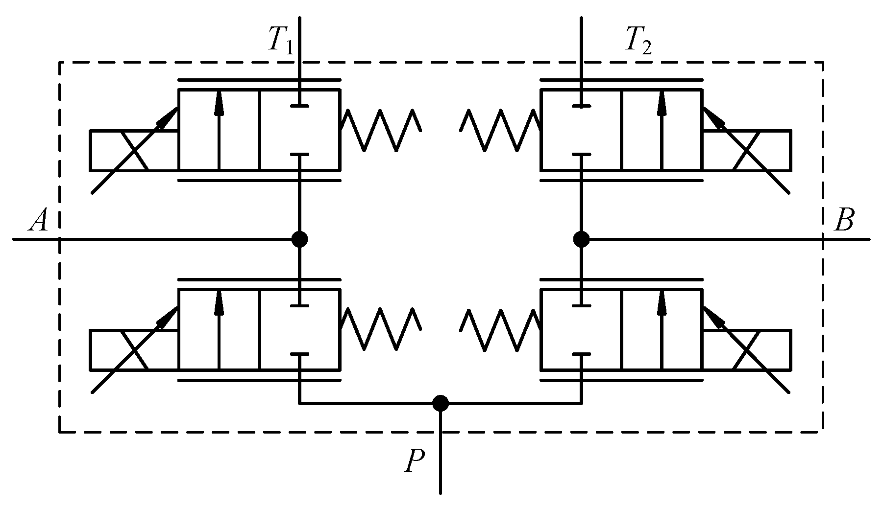
The research objective of this study is the four-spool IM valve manufactured by Jiangsu Advanced Construction Machinery Innovation Center Ltd. The diameter of the valve is 32 mm. Figure 1 and Figure 2 are the tested valve and its hydraulic principle respectively. In Figure 2, port P is the oil inlet connected to the pump, port T1 and T2 are the oil outlet connected to the tank, port A and B are the oil ports connected to the load. The valve can be simplified into four 2/2 spool valves. Negative coverage of each spool valve is 2.5 mm, and the maximum stroke of the spool is 14.5 mm. There are primarily two working modes in the valve, one case is the oil flow through the PB and the AT1, another case is the oil flow through the PA and the BT2. The two oil loops are symmetrical except for machining errors. Therefore, only one case needs to be taken into account in our study.

2.2. Data Generation by Experiments

A dataset is needed in the development of data-based method. In our study, we generated the dataset by experiments of the tested valve. First, we need to determine the variables that need to be collected. The flow rate through the hydraulic valve is calculated by Equation (1), as follows:
Q = C d A 2 ( p 1 p 2 ) ρ
where Q is the flow rate, Cd is the discharge coefficient, A is the flow area, p1 is the pre-valve pressure, p2 is the post-valve pressure, and ρ is the density of oil.
It can be seen that the flow rate in the valve is affected by the variables contained in the Equation (1). Except for the pressure p1 and p2, other parameters cannot be measured directly. But the Cd, A and ρ are related to the valve opening and oil temperature which can be measured easily. Therefore, the oil temperature, oil pressure, valve opening and flow rate were determined as the collected variables.
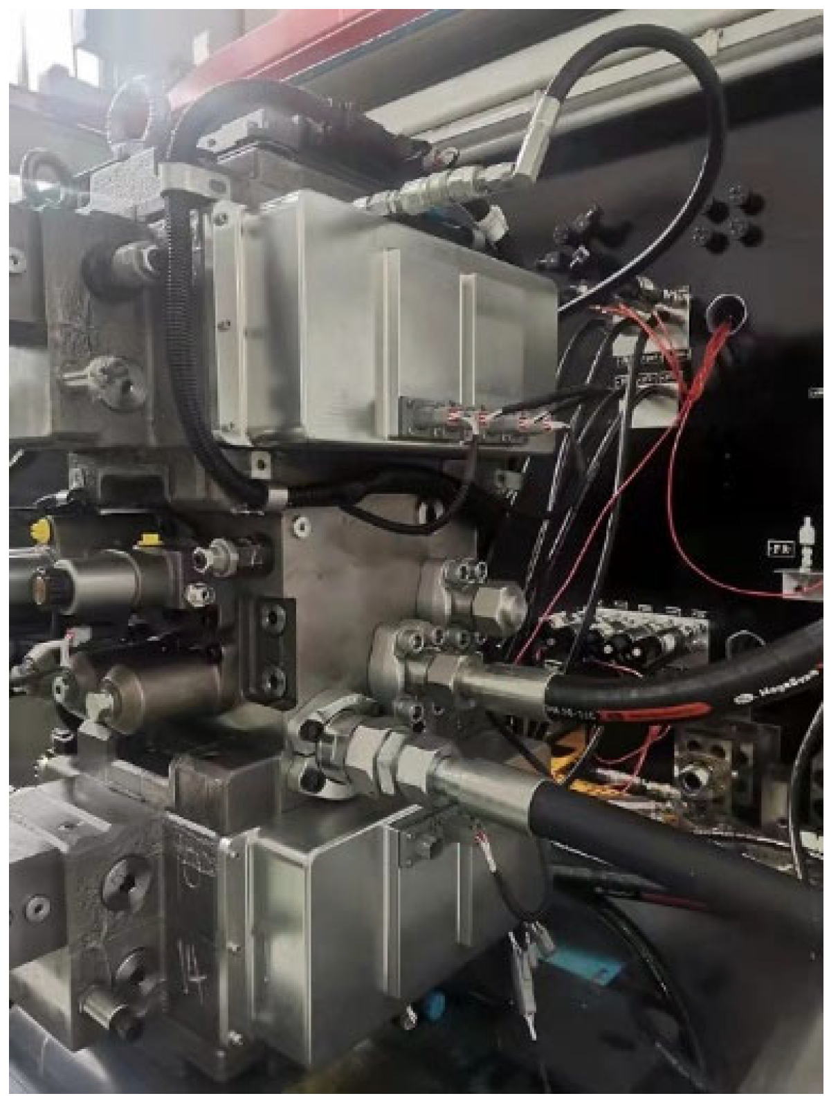
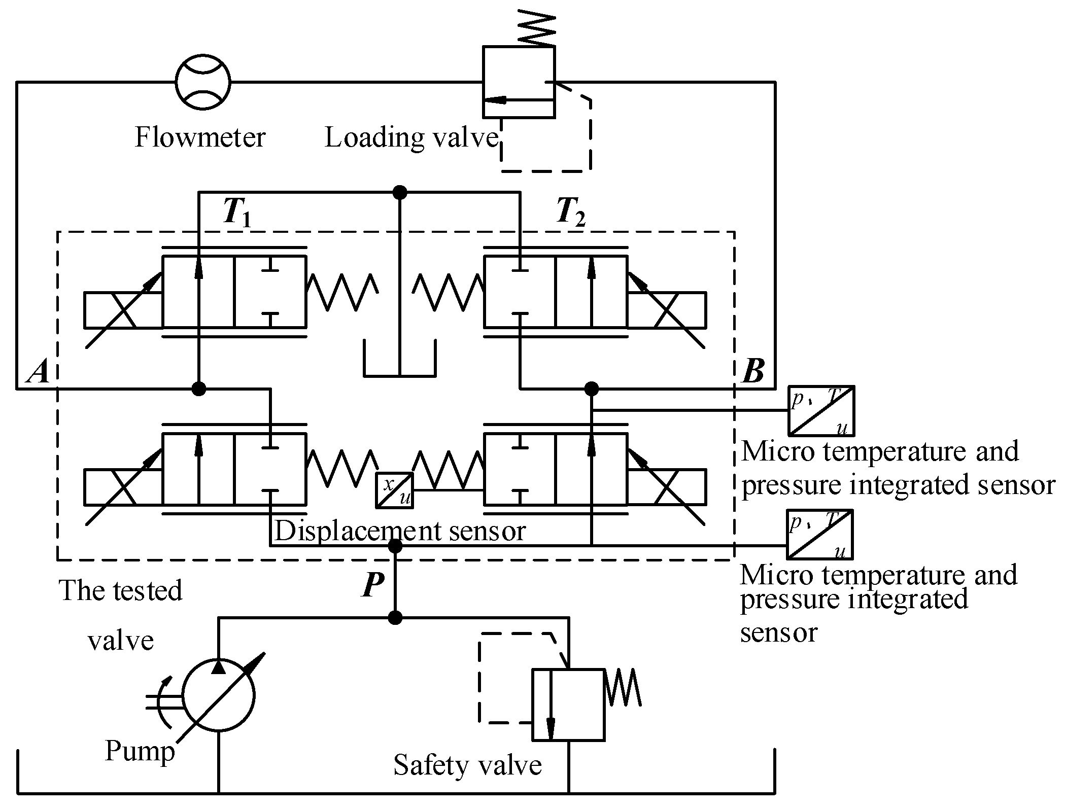
Then we took the multi-channel valve test platform of Jiangsu Advanced Construction Machinery Innovation Center Ltd which is shown in Figure 3 as the foundation, and built the test system whose experimental principle is shown in Figure 4.
In the experiments, the oil provided by the pump went through the PB and the AT1 circuit of the tested valve and then returned to the tank. The temperature, pressure, flow rate of oil and valve opening in the PB valve cavity have been obtained accurately by the flowmeter, the micro temperature and pressure integrated sensors and the displacement sensor connected to the valve stem when the experiments operated.
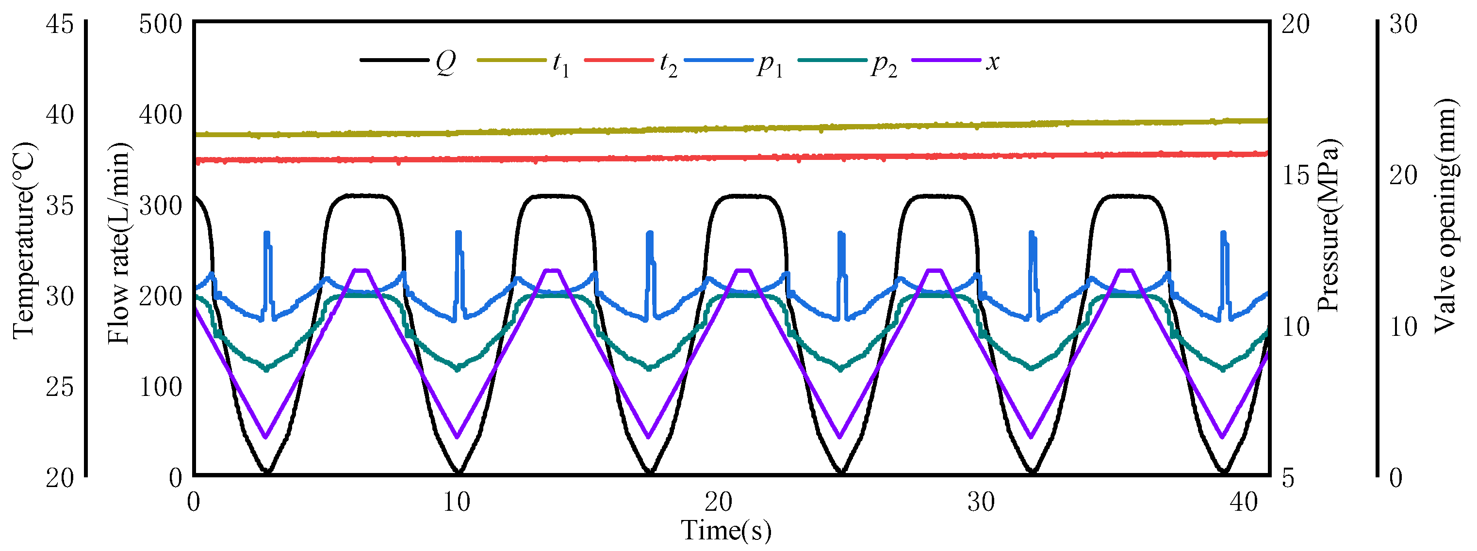
The dataset generated by the experiments is shown in Figure 5. The dataset contains six features, namely P port temperature, B port temperature, P port pressure, B port pressure, valve opening, and valve flow rate, with a total of 8244 sets of data. The above six features are described as t1, t2, p1, p2, x and Q respectively for the convenience. The first 70% of the experimental dataset were used to train the model, and the remaining 30% of the dataset were utilized for test and evaluation in our study.

3. Dataset Analysis and Input Selection

3.1. Dataset Analysis

The dataset collected from the test valve experiments contains 6 features. Table 1 displays the descriptive statistics of different features. MIN, MAX and AVG represent the minimum, maximum and average values for each feature respectively. CV is the coefficient of variation, equal to the standard deviation divided by the mean value, which is utilized to compare the volatility of different dimensional data. The ranges of features are: t1 (38.591–39.602 °C), t2 (37.142–38.841 °C), p1 (10.090–13.042 MPa), p2 (8.462–10.964 MPa), x (2.503–13.543 mm), Q (1.453–307.942 L/min). The throttling effect of the valve port would cause the oil temperature to rise. But the increase of t1 and t2 is significantly slight owing to the short sampling time. The pressure pulsations and losses would been generated as a result of the turbulence in the valve. Hence the CV of p2 is larger than that of p1, but the minimum, maximum and average values of p2 are lower than those of p1.

3.2. Input Selection

Selecting features with the strongest prediction power in dataset is a crucial step before performing ML method. In our study, the Pearson Correlation was utilized as the metric of prediction power for input selection. The Pearson Correlation Coefficient is calculated by Equation (2), as follows:
r = i = 1 n ( x i x ¯ ) ( y i y ) ¯ i = 1 n ( x i x ¯ ) 2 i = 1 n ( y i y ¯ ) 2
where r is the Pearson Correlation Coefficient, n is the number of samples, xi and yi are the points in different samples, x ¯ and y ¯ are the mean of individual samples.
The output of the coefficient ranges from −1 to +1, with larger absolute values indicating stronger correlations. A change in scale of the two variables has no effect on the coefficient.
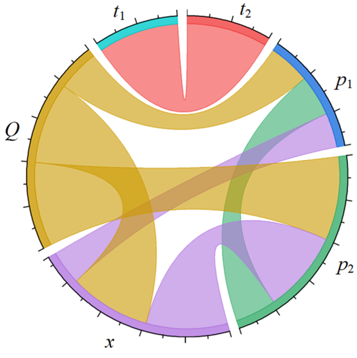
Pearson correlation coefficients between different features were calculated according to Equation (2), and the chord diagram is given in Figure 6. The r values between x, p2 and Q are 0.970 and 1 respectively, showing relatively high correlation. Hence, x and p2 have greater ability to calculate the flow rate in the valve. Thus x and p2 were selected as the input variables of the regression model in this study. In addition, there is a high correlation between x and p2, with the r reaching 0.974, indicating the multicollinearity among the selected input possibly.

4. Regression Models and Hyperparameters Optimization

4.1. Machine Learning Techniques

Since the data collected are labeled previously, supervised regression models are suitable for our research.

4.1.1. Linear Regression

Linear Regression (LR) employs a linear regression equation to fit the regularity of variables [22,23]. The LR assumption function and the cost function based on the ordinary least square method are calculated by Equations (3) and (4) respectively, as follows:
h ( x ) = β 0 + β 1 x 1 + β 2 x 2 + β 3 x 3 + + β n x n
J ( β ) = 1 2 m i = 1 m ( h θ ( x ( i ) ) y ( i ) ) 2
where x is the independent variables, β is the coefficient vector, m is the number of samples, and y is the target value.
The near-linear relationships among the independent variables called multicollinearity affect the results of LR seriously. Ridge adds a penalty to the ordinary least square to reduce the incidence of multicollinearity. The cost function of Ridge is calculated by Equation (5), as follows:
J ( β ) = 1 2 m i = 1 m ( h θ ( x ( i ) ) y ( i ) ) 2 + α j = 1 p β j 2
where α is the regularization parameter, and p is the number of independent variables.

4.1.2. K-Nearest Neighbor

K-nearest Neighbor (KNN) is an instance-based learning method. The model finds the k nearest neighbors in a given sample space, and takes the average or weighted average of the neighbors as the calculated values. The Euclidean distance is invoked as a metric of weight in the model. The distance is calculated by Equation (6), as follows:
E u c l i d e a n     d i s t a n c e = i = 1 n ( x i y i ) 2
where x and y are two points with n number of feature i.

4.1.3. Decision Tree

Decision Tree (DT) is good at expressing the association between data. The Classification and Regression Tree (CART) algorithm was first proposed by Breiman in 1984 [24]. CART is suitable for consecutive and multi-feature variables with binary segmentation. Meanwhile, this algorithm has simple extraction rules, high accuracy and strong interpretability [25]. Hence, the CART was utilized in DT prediction model of our study.

4.1.4. Random Forest

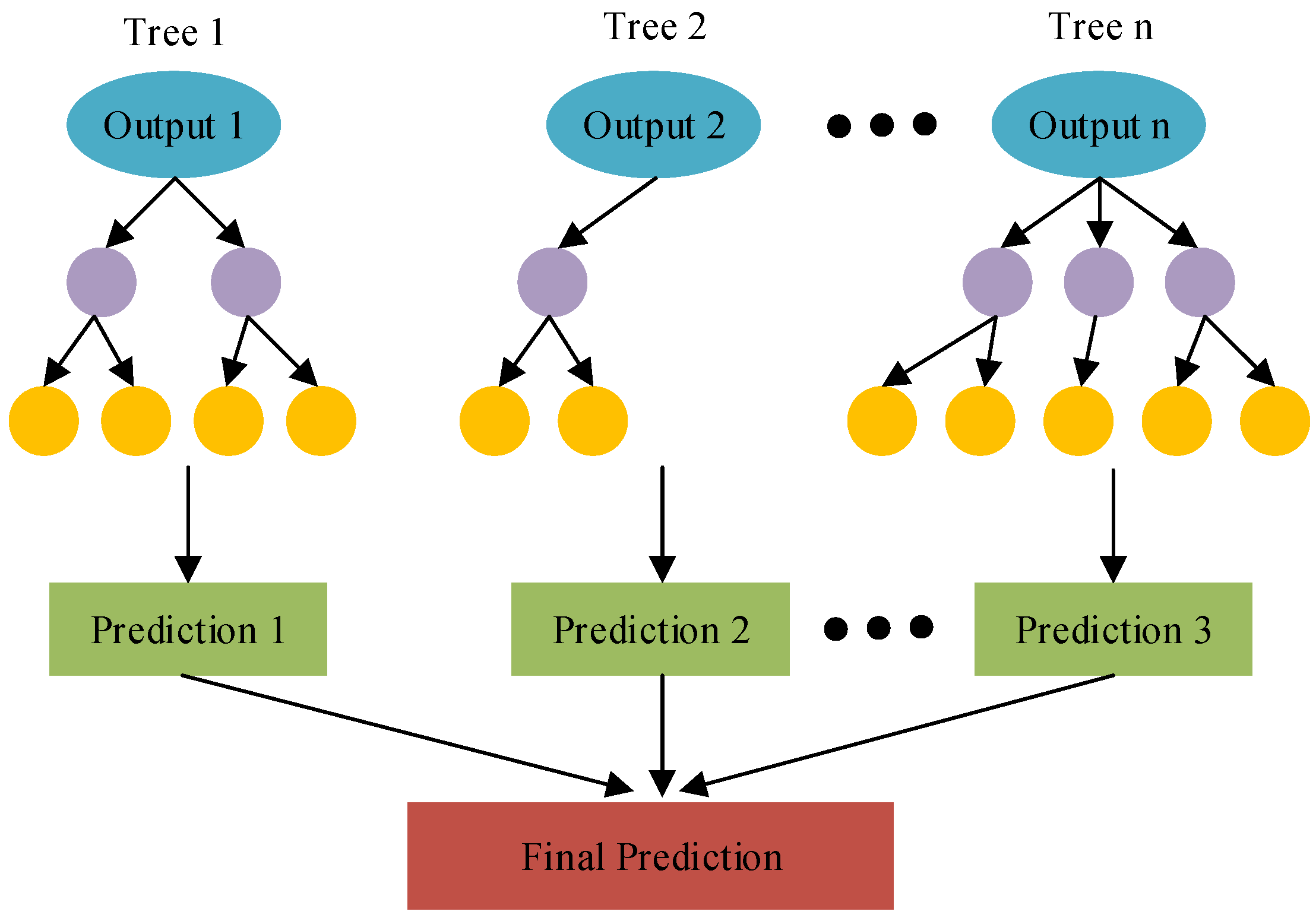
Random Forest (RF) uses multiple trees for ensemble integrated learning. RF could avoid the shortcoming of overfitting in DT effectively [26]. RF calculates and compares multiple decision trees, and picks up the average of the outputs of all trees as the calculated values. The performance of RF produces better with the number of decision trees increases, but the calculation time will become longer. Figure 7 displays the calculation process of RF.

4.1.5. Support Vector Regression

For a given dataset of the independent variable x, Support Vector Regression (SVR) determines a linear function with dependent variable y within a given tolerance [27]. The function is calculated by Equation (7), as follows:
y = w x + b
where w is the slope, and b is the intercept.
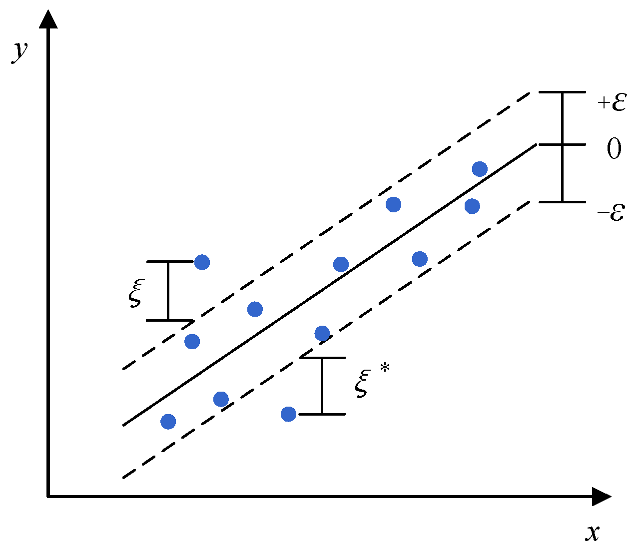
In order to ensure the flatness of line represented by Equation (7), it is necessary to find a minimum w. When the accuracy is ε and the relaxation factors are ξ and ξ*, the problem of the estimation in Equation (7) is calculated by Equations (8) and (9), as follows:
minimize 1 2 w 2 + C i = 1 N ( ξ i + ξ i * )
y i w x i b ε + ξ i w x i + b y i ε + ξ i * ξ i , ξ i * > 0
where C is the trade-off between the w and the deviation of ξ, ξ*.
Figure 8 shows the principle that SVR finds the linear function in terms of Equations (7)–(9).
For a nonlinear dataset, the kernel function is used to transform the dataset into a linear form. The kernel function is calculated by Equation (10), as follows:
y = i = 1 n ( α i α i * ) · K ( x i , x ) + b
where αi and α i * are Lagrange multipliers, K(xi, x) is the kernel.
The radial basis function (RBF) is commonly used as kernel function which is calculated by Equation (11), as follows:
K ( x , x ) = exp ( γ x x 2 )
where γ is a free parameter.
The hyper parameters of SVR (RBF) are C and γ, which should be hunted carefully.

4.1.6. Artificial and Deep Neural Network

Artificial Neural Network (ANN) is a forward network with one hidden layer, which approximates the nonlinear mapping of multi-variate functions through multiple composites of unary functions [28]. The difference between ANN and Deep Neural Network (DNN) is the number of hidden layers. Figure 9 displays the basic structure of ANN and DNN.

4.2. Hyperparameters Optimization

Grid search and random search are two widely used hyperparameters optimization methods. The grid search can traverse all parameters combinations, so the computational cost is high when the number of parameters is large [29]. The random search randomly searches for possible parameters combinations within the specified parameter range, which can significantly reduce the computational cost. In our study, both methods are used for hyper parameter optimization. Depending on the number of hyper parameters, the grid search was used for Ridge, KNN, DT, RF, SVR, and the random search was utilized for ANN and DNN.
In Ridge, alpha (α) was searched from 10−10 to 10. In KNN, k was searched in the range of 1–50. In DT, the maximum depth and the minimum leaf nodes are used to control the size and complexity of the tree to avoid overfitting. So in our DT model, the maximum depth ranged from 10 to 100, and the minimum leaf nodes ranged from 1 to 5. In RF, besides the maximum depth and the minimum leaf nodes, the number of trees needs to be considered to avoid overfitting. The number of trees was searched in the range of 10–100, the maximum depth ranged from 10 to 100, the minimum leaf nodes ranged from 1 to 5. In SVR, the value of C will affect the generalization ability of the model. We searched C from 2−5 to 25, and the range of gamma was 2−5–25. In ANN and DNN, the number of neurons in each hidden layer was searched in the range of 1–2 times the number of neurons in the previous layer, the activation function was searched in logistic, tanh and relu, the solver was adam, the batch size was ranged from 100 to 1000, the range of learning rate was 10−5–10−1, the maximum iterations were 20,000. When the accuracy rate was no longer improved, the training was stopped early to avoid overfitting.
K-fold cross-validation was utilized to find the hyperparameters with the best generalization performance of our models. At each iteration, a different subset was selected for testing and the remaining K-1 subsets were used for training. In this study, the K value was 10. Table 2 displays the hyper parameters searched for the models.

5. Results and Discussion

5.1. Performance Evaluation Criteria of Models

In the study, four statistical measures were adopted for the performance evaluation of our models, as follows:
(i)
Coefficient of determination, R2. High R2 value indicates a good performance of the model.
R 2 = 1 1 n ( y i y ^ i ) 2 1 n ( y i y ¯ i ) 2
where yi and ŷi are the observation and calculation values in the i-th step.
(ii)
Mean absolute error, MAE. The mean absolute error is used to measure the accuracy of continuous variables.
MAE = 1 n i = 1 n y i y ^ i
(iii)
Root mean square error, RMSE. The root mean square error is determined by the square root of the sum of the differences between observation and prediction values. The situation that the root mean square error on the training set is lower the error on the test set indicates overfitting possibly.
RMSE = 1 n i = 1 n ( y i y ^ i ) 2
(iv)
Mean absolute percentage error, MAPE. The mean absolute percentage error can avoid positive and negative errors canceling each other out.
MAPE = 100 % n i = 1 n y ^ i y i y i

5.2. Comparison of Regression Models

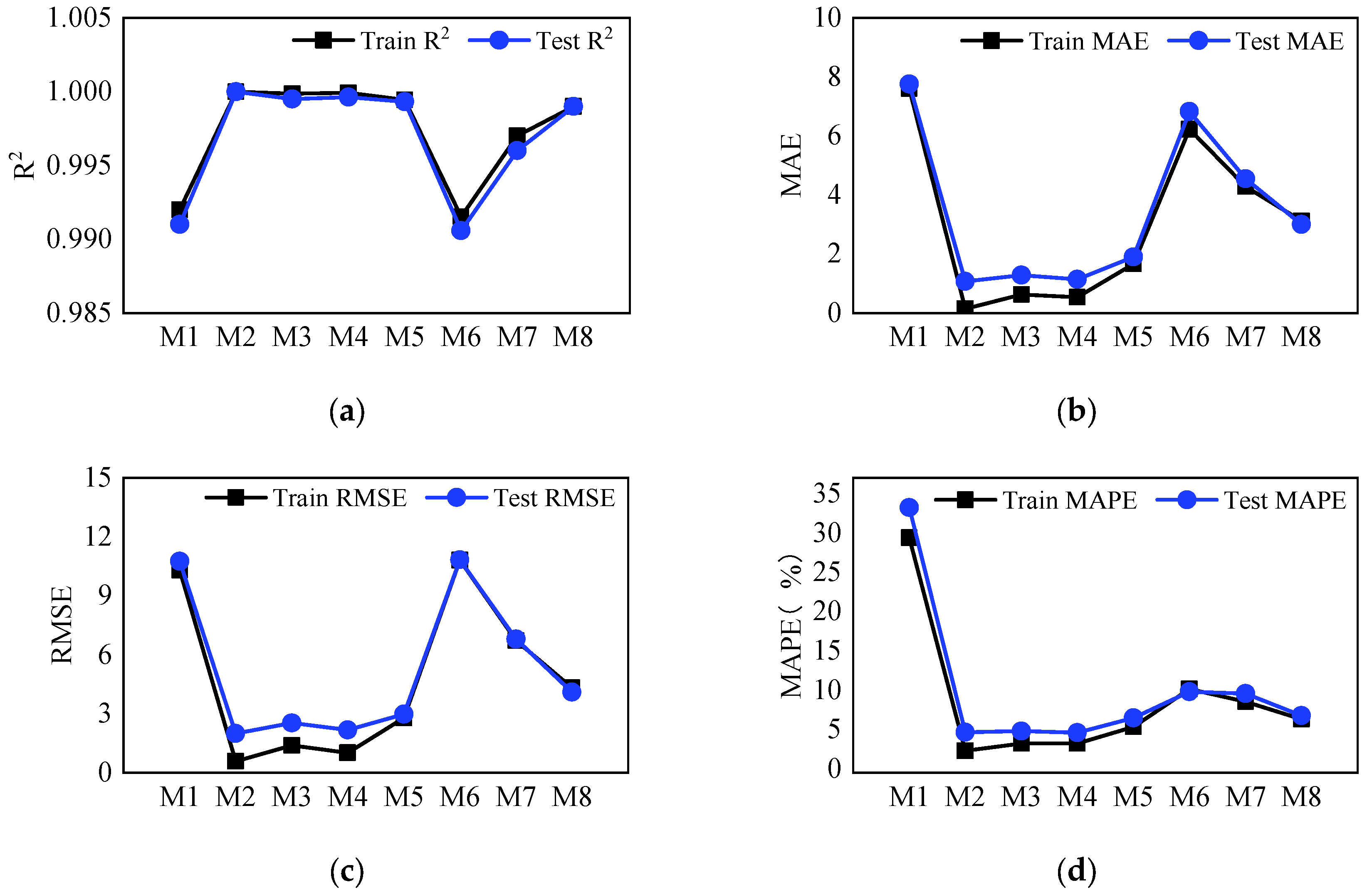
In the previous section, we obtained the optimal hyperparameters of each model. The models were trained and tested in this section. Figure 10 shows the performance evaluation criteria of each model on the training set and test set. M1–8 represent Ridge, KNN, DT, RF, SVR, ANN and DNN with two and three hidden layers respectively.
In the training set, KNN, DT and RF had the highest R2, which was 1. The R2 of SVR and DNN with three hidden layers was next. The R2 of ANN and DNN with two hidden layers were less than others. The LR model’s R2 was just 0.992, which may be caused by collinearity between p2 and x. Compared with other models, KNN DT and RF had smallest MAE, RMSE and MAPE at the same time. SVR and DNN with three hidden layers was the second. The performance of Ridge, ANN and DNN with two hidden layers measured by MAE, RMSE and MAPE was worst.
In the test set, KNN also had highest R2. The next models were DT, RF, SVR and DNN with 3 hidden layers. The R2 of Ridge, ANN and DNN with 2 hidden layers was lower than other models. The MAE, RMSE and MAPE of KNN DT and RF were lower than others. SVR and DNN with three hidden layers were next. Ridge, ANN and DNN with two hidden layers were the poorest models.
In the whole dataset, KNN, DT and RF had the highest R2 and lowest MAE, RMSE, MAPE than other models. But the RMSE of them in the training set was greatly less than in the test set, which indicated serious overfitting. Almost no overfitting occurred in the LR, ANN and DNN with two hidden layers, but the accuracy of them was much lower than other models. Only SVR and DNN with three hidden layers had high accuracy and little overfitting simultaneously.
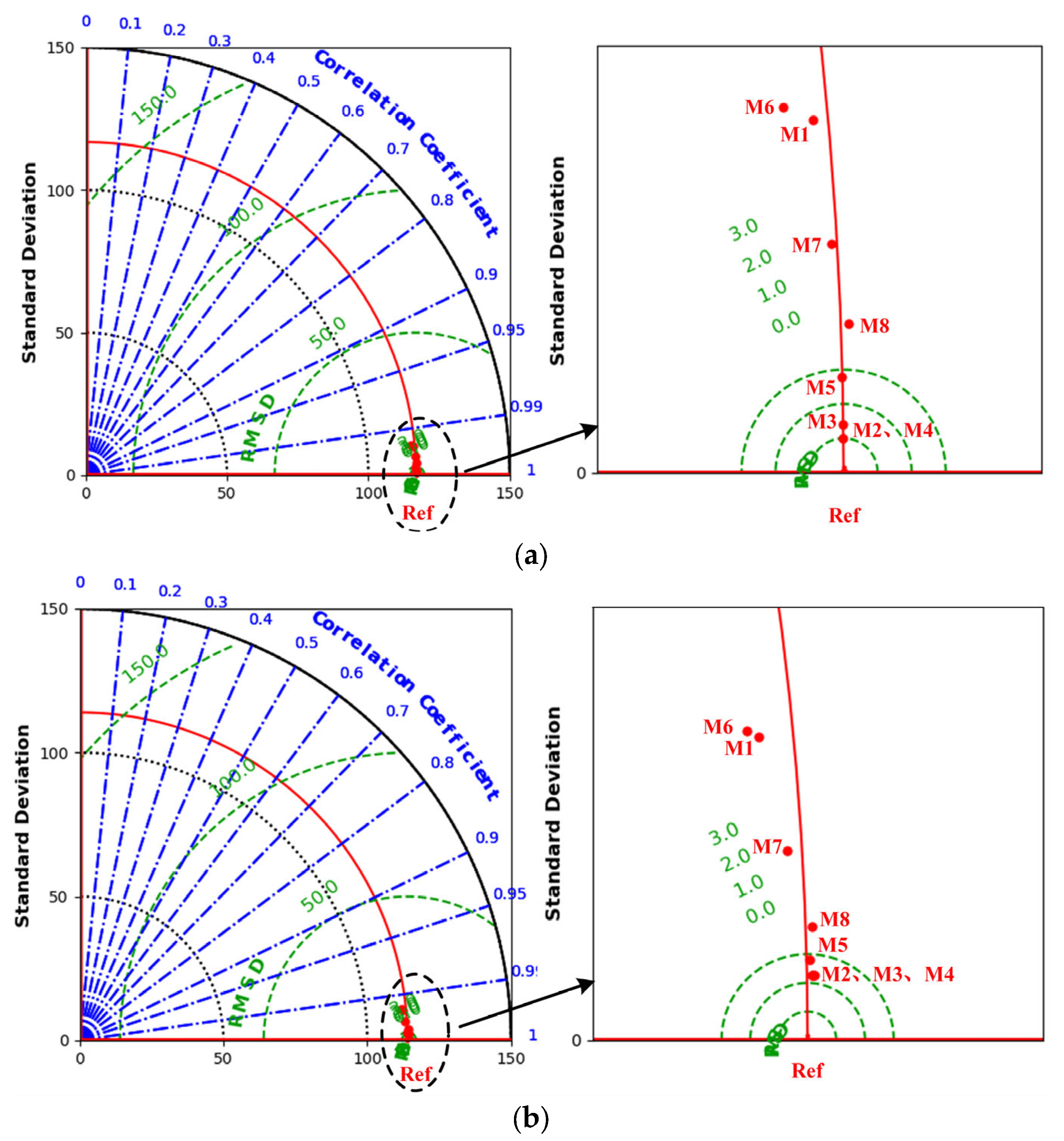
Taylor diagram summarizes how well the outcome of models match observations graphically [30]. The similarity of the models to the reference is displayed according to the correlation, the central root mean square error (CRMSE) and the standard deviation, where the correlation is calculated in the same way as Equation (2). Figure 11 is the Taylor diagram of M1–M8 on the training set and test set respectively. Compared with other models, the KNN, DT and RF had higher correlation coefficient, smaller CRMSE and standard deviation compared with the actual referenced flow rate in the valve on the entire dataset. The SVR and DNN with three hidden layers had moderate correlation coefficient and CRMSE. In addition, the standard deviation values of these two models were close to zero in training set and test set respectively, indicating that the models results were consistent with actual values on the whole dataset.
Overall, SVR and DNN with three hidden layers performed best in the trade-off of accuracy and overfitting. The models accuracy represented by the MAPE on the entire dataset was 3.926% and 4.535% respectively.

6. Conclusions

In view of the difficulty of accurate estimation of the in-valve flow rate under space constraints at present, this study took the four-spool IM valve as the research object and proposed a data-based flow rate prediction method. IM valve experiments have been carried out to generate labeled data. Then the pre-valve pressure, post-valve pressure and valve opening were chosen as input variables according to the prediction power. Different data-based models including machine learning and deep learning were developed and compared. The results indicate that SVR and DNN with three hidden layers performed best in the trade-off of accuracy and overfitting. The models’ MAPE on the entire dataset was 3.926% and 4.535% respectively.
Our study also have some limitations. The sample size will affect the accuracy of ML method. It’s significantly essential to train the ML models based on more samples in the future. However, this study provides the possibility for high-precision flow rate prediction of multi-way valve under limited installation space, and has definite reference value for promoting digitalization, networking and smartness of the hydraulic system of construction machinery.

Author Contributions

Conceptualization, W.R.; methodology, W.R.; software, W.R.; validation, W.R.; formal analysis, W.R.; investigation, W.R.; resources, W.S., H.S., C.L., X.L., Y.H. and H.J.; data curation, W.R.; writing—original draft preparation, W.R.; writing—review and editing, W.R., W.S. and H.W.; visualization, W.R.; supervision, W.S.; project administration, W.S.; funding acquisition, W.S. All authors have read and agreed to the published version of the manuscript.

Funding

This research was funded by National Key R&D Program of China, grant number 2020YFB2009802.

Data Availability Statement

Not applicable.

Conflicts of Interest

The authors declare no conflict of interest.

References

  1. Lin, T.L.; Chen, Q.; Ren, H.L.; Huang, W.P.; Chen, Q.H.; Fu, S.J. Review of boom potential energy regeneration technology for hydraulic construction machinery. Renew. Sust. Energ. Rev. 2017, 79, 358–371. [Google Scholar] [CrossRef]
  2. Do, T.C.; Dang, T.D.; Dinh, T.Q.; Ahn, K.K. Developments in energy regeneration technologies for hydraulic excavators: A review. Renew. Sust. Energ. Rev. 2021, 145, 111076. [Google Scholar] [CrossRef]
  3. Xu, B.; Cheng, M. Motion control of multi-actuator hydraulic systems for mobile machineries: Recent advancements and future trends. Front. Mech. Eng. 2018, 13, 151–166. [Google Scholar] [CrossRef]
  4. Quan, L.; Xia, L.; Zhao, B.; Ge, L. Innovation Progress in Research on Gravitational Potential Energy Recovery and Utilization of Hydraulic Driven Mechanical Arm. J. Mech. Eng. 2018, 54, 4–13. [Google Scholar] [CrossRef]
  5. Kailei, L.; Shaopeng, K.; Rongsheng, L. Optimal Metering Mode for Improving Transform Efficiency of Independent Metering System. In Proceedings of the 2019 IEEE 8th International Conference on Fluid Power and Mechatronics (FPM), Wuhan, China, 10–13 April 2019; pp. 1035–1041. [Google Scholar]
  6. Zhang, X.G.; Qiao, S.F.; Quan, L.; Ge, L. Velocity and Position Hybrid Control for Excavator Boom Based on Independent Metering System. IEEE Access 2019, 7, 71999–72011. [Google Scholar] [CrossRef]
  7. Zatopa, A.; Walker, S.; Menguc, Y. Fully Soft 3D-Printed Electroactive Fluidic Valve for Soft Hydraulic Robots. Soft Robot. 2018, 5, 258–271. [Google Scholar] [CrossRef]
  8. Pan, M.; Plummer, A.; El Agha, A. Theoretical and Experimental Studies of a Switched Inertance Hydraulic System in a Four-Port High-Speed Switching Valve Configuration. Energies 2017, 10, 780. [Google Scholar] [CrossRef] [Green Version]
  9. Kong, L.X.; Wei, W.; Yan, Q.D. Application of flow field decomposition and reconstruction in studying and modeling the characteristics of a cartridge valve. Eng. Appl. Comp. Fluid Mech. 2018, 12, 385–396. [Google Scholar] [CrossRef]
  10. Dempster, W.; Elmayyah, W. Two phase discharge flow prediction in safety valves. Int. J. Pressure Vessels Pip. 2013, 110, 61–65. [Google Scholar] [CrossRef] [Green Version]
  11. Sekar, V.; Jiang, Q.H.; Shu, C.; Khoo, B.C. Fast flow field prediction over airfoils using deep learning approach. Phys. Fluids 2019, 31, 057103. [Google Scholar] [CrossRef]
  12. Choi, D.; An, Y.; Lee, N.; Park, J.; Lee, J. Comparative Study of Physics-Based Modeling and Neural Network Approach to Predict Cooling in Vehicle Integrated Thermal Management System. Energies 2020, 13, 5301. [Google Scholar] [CrossRef]
  13. Sun, Y.B.; Sun, Q.K.; Qin, K. Physics-Based Deep Learning for Flow Problems. Energies 2021, 14, 7760. [Google Scholar] [CrossRef]
  14. Rao, M.M.; Wang, L.; Chen, C.T.; Xiong, K.; Li, M.F.; Chen, Z.P.; Dong, J.B.; Xu, J.L.; Li, X. Data-Driven State Prediction and Analysis of SOFC System Based on Deep Learning Method. Energies 2022, 15, 3099. [Google Scholar] [CrossRef]
  15. Croitoru, I.; Bogolin, S.V.; Leordeanu, M. Unsupervised Learning of Foreground Object Segmentation. Int. J. Comput. Vis. 2019, 127, 1279–1302. [Google Scholar] [CrossRef] [Green Version]
  16. Zhang, Y.; He, X.F.; Chen, Z.Q.; Bai, Q.; Nolan, A.M.; Roberts, C.A.; Banerjee, D.; Matsunaga, T.; Mo, Y.F.; Ling, C. Unsupervised discovery of solid-state lithium ion conductors. Nat. Commun. 2019, 10, 5260. [Google Scholar] [CrossRef] [Green Version]
  17. Li, Y.F.; Guo, L.Z.; Zhou, Z.H. Towards Safe Weakly Supervised Learning. IEEE Trans. Pattern Anal. Mach. Intell. 2021, 43, 334–346. [Google Scholar] [CrossRef] [PubMed] [Green Version]
  18. Ohri, K.; Kumar, M. Review on self-supervised image recognition using deep neural networks. Knowl. Based Syst. 2021, 224, 107090. [Google Scholar] [CrossRef]
  19. Jia, Z.Y.; Ma, J.W.; Wang, F.J.; Liu, W. Hybrid of simulated annealing and SVM for hydraulic valve characteristics prediction. Expert Syst. Appl. 2011, 38, 8030–8036. [Google Scholar] [CrossRef]
  20. Zhao, S.; Wang, S.; Shang, Y. Fault diagnosis for piston head looseness of aero hydraulic pump. J. Beijing Univ. Aeronaut. Astronaut. 2010, 36, 261–264. [Google Scholar]
  21. Guo, Y.; Zeng, Y.C.; Fu, L.D.; Chen, X.Y. Modeling and Experimental Study for Online Measurement of Hydraulic Cylinder Micro Leakage Based on Convolutional Neural Network. Sensors 2019, 19, 2159. [Google Scholar] [CrossRef] [Green Version]
  22. Jumin, E.; Zaini, N.; Ahmed, A.N.; Abdullah, S.; Ismail, M.; Sherif, M.; Sefelnasr, A.; Ei-Shafie, A. Machine learning versus linear regression modelling approach for accurate ozone concentrations prediction. Eng. Appl. Comp. Fluid Mech. 2020, 14, 713–725. [Google Scholar] [CrossRef]
  23. Korkmaz, M. A study over the general formula of regression sum of squares in multiple linear regression. Numer. Meth. Part Differ. Equ. 2021, 37, 406–421. [Google Scholar] [CrossRef]
  24. Speybroeck, N. Classification and regression trees. Int. J. Public Health 2012, 57, 243–246. [Google Scholar] [CrossRef] [PubMed]
  25. Yang, S.; Guo, J.Z.; Jin, J.W. An improved improved Id3 algorithm for medical data classification. Comput. Electr. Eng. 2018, 65, 474–487. [Google Scholar] [CrossRef]
  26. Breiman, L. Random forests. Mach. Learn. 2001, 45, 5–32. [Google Scholar] [CrossRef] [Green Version]
  27. Ozbas, E.E.; Aksu, D.; Ongen, A.; Aydin, M.A.; Ozcan, H.K. Hydrogen production via biomass gasification, and modeling by supervised machine learning algorithms. Int. J. Hydrogen Energy 2019, 44, 17260–17268. [Google Scholar] [CrossRef]
  28. Valencia, F.; Arcos, H.; Quilumba, F. Prediction of Stress in Power Transformer Winding Conductors Using Artificial Neural Networks: Hyperparameter Analysis. Energies 2021, 14, 4242. [Google Scholar] [CrossRef]
  29. Li, B.; Yao, Q.-Z.; Luo, Z.-M.; Tian, Y.; Wang, W. Gird-pattern method for model selection of support vector machines. Comput. Eng. Applic. 2008, 44, 136–138. [Google Scholar]
  30. Taylor, K.E. Summarizing multiple aspects of model performance in a single diagram. J. Geophys. Res. Atmos. 2001, 106, 7183–7192. [Google Scholar] [CrossRef]
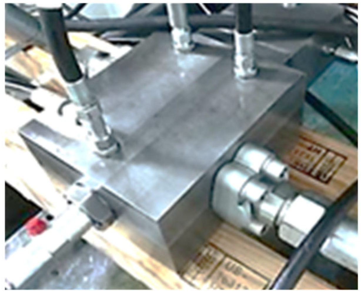
Figure 1. The tested valve.
Energies 15 07699 g001
Figure 2. Hydraulic schematic diagram of the tested valve.
Energies 15 07699 g002
Figure 3. The multi-channel valve test platform.
Energies 15 07699 g003
Figure 4. Diagram of experimental principle.
Energies 15 07699 g004
Figure 5. The dataset generated by the experiments.
Energies 15 07699 g005
Figure 6. Chord diagram representing correlation among features.
Energies 15 07699 g006
Figure 7. The calculation process of RF.
Energies 15 07699 g007
Figure 8. Approximated linear function of SVR with tolerance.
Energies 15 07699 g008
Figure 9. Structure of artificial and deep neural network. (a) Structure of artificial neural network. (b) Structure of deep neural network.
Energies 15 07699 g009
Figure 10. Comparison of models on training set and test set. (a) Comparison of R2. (b) Comparison of MAE. (c) Comparison of RMSE. (d) Comparison of MAPE.
Energies 15 07699 g010
Figure 11. Taylor diagram of different regression models. (a) Performance of M1–M8 on the training set. (b) Performance of M1–M8 on the test set.
Energies 15 07699 g011
Table 1. The descriptive statistics of different features.
Descriptive StatisticsMINMAXAVGCV
t1 (°C)38.59139.60239.0810.010
t2 (°C)37.14238.84137.4900
p1 (MPa)10.09013.04210.9220.050
p2 (MPa)8.46210.9649.8210.091
X (mm)2.50313.5438.0400.410
Q (L/min)1.453307.942167.7940.692
Table 2. Hyper parameters of models.
RidgeKNNDTRFSVRANNDNN (H = 2)DNN (H = 3)
Hyper-parametersA = 10−4K = 8max_depth = 20
min_leaf_nodes = 4
max_depth = 10
min_leaf_nodes = 1
trees = 40
C = 32
Γ = 2
h1 = 5
activation = tanh
batch_size = 400
learning_rate = 0.01
h1 = 4
h2 = 7
activation = tanh
batch_size = 100
learning_rate = 0.01
h1 = 6
h2 = 11
h3 = 1
activation = tanh
batch_size = 200
learning_rate = 0.01
Publisher’s Note: MDPI stays neutral with regard to jurisdictional claims in published maps and institutional affiliations.