
Physics-Informed Neural Network Solution of Point Kinetics Equations for a Nuclear Reactor Digital Twin


Abstract

1. Introduction
1.1. Digital Twin for Nuclear Reactor Monitoring
1.2. Review of Prior Work on PINNs
2. Theory of Physics-Informed Neural Network (PINN)
2.1. Surrogate Network Implementation with Fully Connected Neural Networks (FNNs)
2.2. Automatic Differentiation for Residual Network
2.3. Enforcement of Initial and Boundary Conditions
2.4. Loss Function and Metrics for Evaluation
2.5. Activation Function
2.6. Optimization
2.7. Initialization
3. Point Kinetics Equations (PKEs)
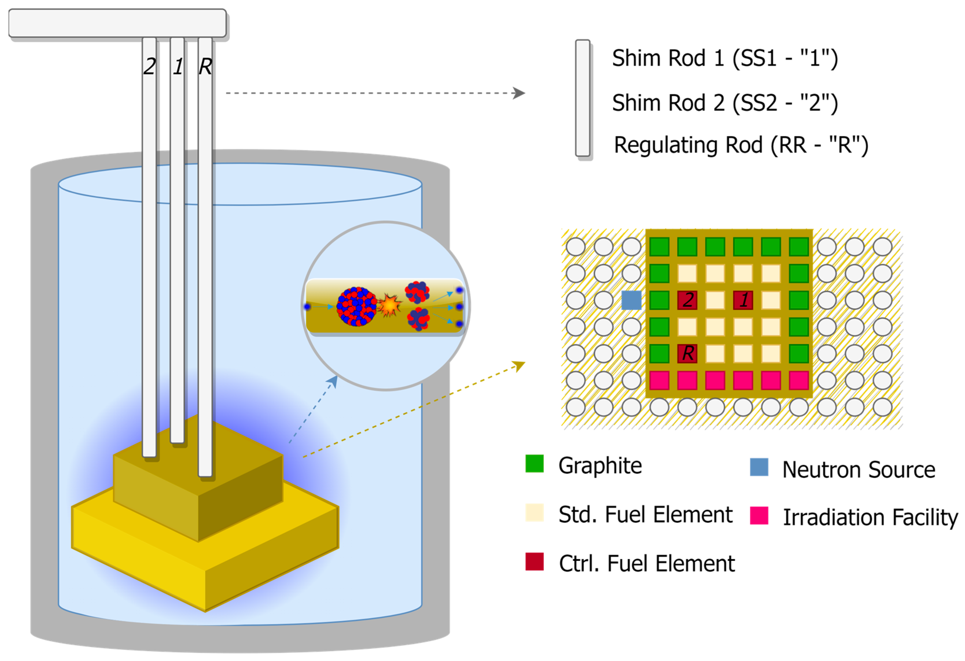
4. Purdue University Reactor Number One (PUR-1)
5. PINN Solution of the PKE Model of PUR-1
5.1. PINN Model Development and Training
5.2. PINN Solution of PKEs
6. Conclusions
Author Contributions
Funding
Data Availability Statement
Acknowledgments
Conflicts of Interest
References
- Kochunas, B.; Huan, X. Digital Twin Concepts with Uncertainty for Nuclear Power Applications. Energies 2021, 14, 4235. [Google Scholar] [CrossRef]
- Kim, C.; Dinh, M.-C.; Sung, H.-J.; Kim, K.-H.; Choi, J.-H.; Graber, L.; Yu, I.-K.; Park, M. Design, Implementation, and Evaluation of an Output Prediction Model of the 10 MW Floating Offshore Wind Turbine for a Digital Twin. Energies 2022, 15, 6329. [Google Scholar] [CrossRef]
- Li, Y.; Yang, J. Meta-Learning Baselines and Database for Few-Shot Classification in Agriculture. Comput. Electron. Agric. 2021, 182, 106055. [Google Scholar] [CrossRef]
- Pylianidis, C.; Snow, V.; Overweg, H.; Osinga, S.; Kean, J.; Athanasiadis, I.N. Simulation-Assisted Machine Learning for Operational Digital Twins. Environ. Model. Softw. 2022, 148, 105274. [Google Scholar] [CrossRef]
- Lagaris, I.E.; Likas, A.; Fotiadis, D.I. Artificial Neural Networks for Solving Ordinary and Partial Differential Equations. IEEE Trans. Neural Netw. 1998, 9, 987–1000. [Google Scholar] [CrossRef] [PubMed]
- Raissi, M.; Perdikaris, P.; Karniadakis, G.E. Physics Informed Deep Learning (Part I): Data-driven Solutions of Nonlinear Partial Differential Equations. arXiv 2017, arXiv:1711.10561. [Google Scholar]
- Raissi, M.; Perdikaris, P.; Karniadakis, G.E. Physics Informed Deep Learning (Part II): Data-driven Discovery of Nonlinear Partial Differential Equations. arXiv 2017, arXiv:1711.10566. [Google Scholar]
- Karniadakis, G.E.; Kevrekidis, I.G.; Lu, L.; Perdikaris, P.; Wang, S.; Yang, L. Physics-Informed Machine Learning. Nat. Rev. Phys. 2021, 3, 422–440. [Google Scholar] [CrossRef]
- Cai, S.; Wang, Z.; Wang, S.; Perdikaris, P.; Karniadakis, G.E. Physics-Informed Neural Networks for Heat Transfer Problems. J. Heat Transf. 2021, 143, 060801. [Google Scholar] [CrossRef]
- Cai, S.; Mao, Z.; Wang, Z.; Yin, M.; Karniadakis, G.E. Physics-Informed Neural Networks (PINNs) for Fluid Mechanics: A Review. Acta Mech. Sin. 2021, 37, 1727–1738. [Google Scholar] [CrossRef]
- Haghighat, E.; Raissi, M.; Moure, A.; Gomez, H.; Juanes, R. A Physics-Informed Deep Learning Framework for Inversion and Surrogate Modeling in Solid Mechanics. Comput. Methods Appl. Mech. Eng. 2021, 379, 113741. [Google Scholar] [CrossRef]
- Prantikos, K.; Tsoukalas, L.H.; Heifetz, A. Physics-Informed Neural Network Solution of Point Kinetics Equations for Development of Small Modular Reactor Digital Twin. In Proceedings of the 2022 American Nuclear Society Annual Meeting, Anaheim, CA, USA, 12–16 June 2022. [Google Scholar] [CrossRef]
- Lu, L.; Meng, X.; Mao, Z.; Karniadakis, G.E. DeepXDE: A Deep Learning Library for Solving Differential Equations. SIAM Rev. 2021, 63, 208–228. [Google Scholar] [CrossRef]
- Sirignano, J.; Spiliopoulos, K. DGM: A Deep Learning Algorithm for Solving Partial Differential Equations. J. Comput. Phys. 2018, 375, 1339–1364. [Google Scholar] [CrossRef]
- Koryagin, A.; Khudorozkov, R.; Tsimfer, S. PyDEns: A python framework for solving differential equations with neural networks. arXiv 2019, arXiv:1909.11544. [Google Scholar]
- Chen, F.; Sondak, D.; Protopapas, P.; Mattheakis, M.; Liu, S.; Agarwal, D.; Di Giovanni, M. NeuroDiffEq: A Python Package for Solving Differential Equations with Neural Networks. JOSS 2020, 5, 1931. [Google Scholar] [CrossRef]
- Zubov, K.; McCarthy, Z.; Ma, Y.; Calisto, F.; Pagliarino, V.; Azeglio, S.; Bottero, L.; Luján, E.; Sulzer, V.; Bharambe, A.; et al. NeuralPDE: Automating Physics-Informed Neural Networks (PINNs) with Error Approximations. arXiv 2021, arXiv:2107.09443. [Google Scholar]
- Xu, K.; Darve, E. ADCME: Learning Spatially-Varying Physical Fields Using Deep Neural Networks. arXiv 2020, arXiv:2011.11955. [Google Scholar]
- Rudy, S.; Alla, A.; Brunton, S.L.; Kutz, J.N. Data-Driven Identification of Parametric Partial Differential Equations. SIAM J. Appl. Dyn. Syst. 2019, 18, 643–660. [Google Scholar] [CrossRef]
- Raissi, M.; Perdikaris, P.; Karniadakis, G.E. Physics-Informed Neural Networks: A Deep Learning Framework for Solving Forward and Inverse Problems Involving Nonlinear Partial Differential Equations. J. Comput. Phys. 2019, 378, 686–707. [Google Scholar] [CrossRef]
- Han, J.; Jentzen, A.; Weinan, E. Solving High-Dimensional Partial Differential Equations Using Deep Learning. Proc. Natl. Acad. Sci. USA 2018, 115, 8505–8510. [Google Scholar] [CrossRef]
- Wiering, M.; van Otterlo, M. (Eds.) Reinforcement Learning. In Adaptation, Learning, and Optimization; Springer: Berlin/Heidelberg, Germany, 2012; Volume 12, ISBN 9783642276446. [Google Scholar]
- Ji, W.; Qiu, W.; Shi, Z.; Pan, S.; Deng, S. Stiff-PINN: Physics-Informed Neural Network for Stiff Chemical Kinetics. J. Phys. Chem. A 2021, 125, 8098–8106. [Google Scholar] [CrossRef] [PubMed]
- Schiassi, E.; De Florio, M.; Ganapol, B.D.; Picca, P.; Furfaro, R. Physics-Informed Neural Networks for the Point Kinetics Equations for Nuclear Reactor Dynamics. Ann. Nucl. Energy 2022, 167, 108833. [Google Scholar] [CrossRef]
- Akins, A.; Wu, X. Using Physics-Informed Neural Networks to solve a System of Coupled Nonlinear ODEs for a Reactivity Insertion Accident. In Proceedings of the 2022 Physics of Reactors, Pittsburgh, PA, USA, 15–20 May 2022. [Google Scholar]
- Markidis, S. The Old and the New: Can Physics-Informed Deep-Learning Replace Traditional Linear Solvers? Front. Big Data 2021, 4, 669097. [Google Scholar] [CrossRef]
- Heifetz, A.; Ritter, L.R.; Olmstead, W.E.; Volpert, V.A. A numerical analysis of initiation of polymerization waves. Math. Comput. Model. 2005, 41, 271–285. [Google Scholar] [CrossRef]
- Baydin, A.G.; Pearlmutter, B.A.; Radul, A.A.; Siskind, J.M. Automatic Differentiation in Machine Learning: A Survey. arXiv 2015, arXiv:1502.05767. [Google Scholar]
- Lagari, P.L.; Tsoukalas, L.H.; Safarkhani, S.; Lagaris, I.E. Systematic Construction of Neural Forms for Solving Partial Differential Equations Inside Rectangular Domains, Subject to Initial, Boundary and Interface Conditions. Int. J. Artif. Intell. Tools 2020, 29, 2050009. [Google Scholar] [CrossRef]
- Wang, S.; Teng, Y.; Perdikaris, P. Understanding and Mitigating Gradient Flow Pathologies in Physics-Informed Neural Networks. SIAM J. Sci. Comput. 2021, 43, A3055–A3081. [Google Scholar] [CrossRef]
- Margossian, C.C. A Review of Automatic Differentiation and Its Efficient Implementation. WIREs Data Min. Knowl. Discov. 2019, 9, e1305. [Google Scholar] [CrossRef]
- Eckle, K.; Schmidt-Hieber, J. A Comparison of Deep Networks with ReLU Activation Function and Linear Spline-Type Methods. Neural Netw. 2019, 110, 232–242. [Google Scholar] [CrossRef]
- Kingma, D.P.; Ba, J. Adam: A Method for Stochastic Optimization. arXiv 2017, arXiv:1412.6980. [Google Scholar]
- Blum, A.; Hopcroft, J.E.; Kannan, R. Foundations of Data Science, 1st ed.; Cambridge University Press: New York, NY, USA, 2020; ISBN 9781108755528. [Google Scholar]
- Tsoukalas, L.H.; Uhrig, R.E. Fuzzy and Neural Approaches in Engineering. In Adaptive and Learning Systems for Signal Processing, Communications, and Control; Wiley: New York, NY, USA, 1997; ISBN 9780471160038. [Google Scholar]
- Lewis, E.E. Fundamentals of Nuclear Reactor Physics; Academic Press: Amsterdam, The Netherlands; Boston, MA, USA, 2008; ISBN 9780123706317. [Google Scholar]
- Townsend, C.H. License Power Capacity of the PUR-1 Research Reactor. Master’s Thesis, Purdue University, West Lafayette, IN, USA, 2018. [Google Scholar]
- Pantopoulou, S. Cybersecurity in the PUR-1 Nuclear Reactor. Master’s Thesis, Purdue University, West Lafayette, IN, USA, 2021. [Google Scholar]
- Baudron, A.-M.; Lautard, J.-J.; Maday, Y.; Riahi, M.K.; Salomon, J. Parareal in Time 3D Numerical Solver for the LWR Benchmark Neutron Diffusion Transient Model. J. Comput. Phys. 2014, 279, 67–79. [Google Scholar] [CrossRef][Green Version]
- He, K.; Zhang, X.; Ren, S.; Sun, J. Delving Deep into Rectifiers: Surpassing Human-Level Performance on ImageNet Classification. In Proceedings of the 2015 IEEE International Conference on Computer Vision (ICCV), Washington, DC, USA, 7–13 December 2015; pp. 1026–1034. [Google Scholar]


| Variable | Value (s) | |||||
|---|---|---|---|---|---|---|
| Term | 1 | 2 | 3 | 4 | 5 | 6 |
| 0.000213 | 0.001413 | 0.001264 | 0.002548 | 0.000742 | 0.000271 | |
| 0.01244 | 0.0305 | 0.1114 | 0.3013 | 1.1361 | 3.013 | |
| SS2 (cm) | Reactivity (pcm) | Uncertainty (pcm) |
|---|---|---|
| 0 | −1168.496 | 97 |
| 10 | −983.580 | 74 |
| 20 | −870.513 | 80 |
| 30 | −431.857 | 78 |
| 40 | −31.009 | 90 |
| Step # | Procedure |
|---|---|
| Step 1 | Specify the computational domain using the geometry module. |
| Step 2 | Specify the system of ODEs using the grammar of Tensorflow. |
| Step 3 | Specify the initial conditions using the IC module. |
| Step 4 | Combine the geometry, system of ODEs, and initial conditions together into data.PDE. Specify the training data and the training distribution, and set the number of points to be sampled. |
| Step 5 | Construct a feed-forward neural network using the maps module. |
| Step 6 | Define a Model by combining the system of ODEs problem in Step 4 and the neural network in Step 5. |
| Step 7 | Call Model.compile to set the optimization hyperparameters, such as optimizer and learning rate. The weights in Equation (4) can be set here by loss_weights. |
| Step 8 | Call Model.train to train the network from random initialization. The training behavior can be monitored and modified using callbacks. |
| Step 9 | Call Model.predict to predict the PDE solution at different locations. |
| Variable | Value (%) | ||||
|---|---|---|---|---|---|
| Test Point | 1 | 2 | 3 | 4 | 5 |
| 1.237 | 1.382 | 1.468 | 1.488 | 1.434 | |
| 0.237 | 0.109 | 0.037 | 0.196 | 0.365 | |
| 0.144 | 0.443 | 0.748 | 1.056 | 1.360 | |
| 1.378 | 1.633 | 1.871 | 2.082 | 2.260 | |
| 1.067 | 1.173 | 1.243 | 1.268 | 1.241 | |
| 1.410 | 1.490 | 1.513 | 1.481 | 1.383 | |
| 1.559 | 1.868 | 2.118 | 2.298 | 2.404 | |
| Variable | Value (%) | ||||
| Test Point | 1 | 2 | 3 | 4 | 5 |
| 2.564 | 1.434 | 1.954 | 2.277 | 2.361 | |
| 1.190 | 0.032 | 0.478 | 0.994 | 1.565 | |
| 1.181 | 0.167 | 1.045 | 1.955 | 2.877 | |
| 2.500 | 1.503 | 2.456 | 3.345 | 4.138 | |
| 2.755 | 1.654 | 2.386 | 2.986 | 3.416 | |
| 2.433 | 1.197 | 1.675 | 1.980 | 2.072 | |
| 2.560 | 1.280 | 1.683 | 1.904 | 1.902 | |
| Variable | Value (%) | ||||
|---|---|---|---|---|---|
| Test Point | 1 | 2 | 3 | 4 | 5 |
| 1.841 | 2.630 | 3.971 | 5.424 | 6.747 | |
| 0.787 | 0.551 | 0.436 | 1.779 | 3.276 | |
| 0.256 | 0.915 | 2.397 | 4.249 | 6.248 | |
| 1.665 | 2.473 | 4.083 | 5.996 | 7.963 | |
| 1.761 | 2.413 | 3.824 | 5.476 | 7.107 | |
| 1.645 | 2.205 | 3.457 | 4.891 | 6.257 | |
| 2.076 | 3.014 | 4.469 | 6.022 | 7.452 | |
Publisher’s Note: MDPI stays neutral with regard to jurisdictional claims in published maps and institutional affiliations. |
© 2022 by the authors. Licensee MDPI, Basel, Switzerland. This article is an open access article distributed under the terms and conditions of the Creative Commons Attribution (CC BY) license (https://creativecommons.org/licenses/by/4.0/).
Share and Cite
Prantikos, K.; Tsoukalas, L.H.; Heifetz, A. Physics-Informed Neural Network Solution of Point Kinetics Equations for a Nuclear Reactor Digital Twin. Energies 2022, 15, 7697. https://doi.org/10.3390/en15207697
Prantikos K, Tsoukalas LH, Heifetz A. Physics-Informed Neural Network Solution of Point Kinetics Equations for a Nuclear Reactor Digital Twin. Energies. 2022; 15(20):7697. https://doi.org/10.3390/en15207697
Chicago/Turabian StylePrantikos, Konstantinos, Lefteri H. Tsoukalas, and Alexander Heifetz. 2022. "Physics-Informed Neural Network Solution of Point Kinetics Equations for a Nuclear Reactor Digital Twin" Energies 15, no. 20: 7697. https://doi.org/10.3390/en15207697
APA StylePrantikos, K., Tsoukalas, L. H., & Heifetz, A. (2022). Physics-Informed Neural Network Solution of Point Kinetics Equations for a Nuclear Reactor Digital Twin. Energies, 15(20), 7697. https://doi.org/10.3390/en15207697