1. Introduction
Increasing the proportion of energy from renewable sources is a key element in reducing greenhouse gas emissions and keeping the average global temperature increase below 2 °C compared to pre-industrial levels. In fact, reducing the use of fossil fuels by replacing them with renewable resources contributes to the decarbonization of the energy system.
Energy communities are collective organizations that will help the transition to clean energy. They aim to use energy in the same place where it is produced, sharing it among several citizens and managing storage systems in a smart way. They make it possible to create energy-independent areas, with benefits for citizens and the health of the planet. In this context, photovoltaic (PV) fields play an important role. Predicting their electrical productivity is useful for managing their interconnection within a smart grid [
1]. In order to optimize the operation of energy communities, it is very useful to be able to predict the energy demand of users, the electrical supplies of the generators and the charge levels of the electrical accumulators installed in the area [
2,
3,
4]. Being able to simulate the thermal and electrical behavior of generation systems as a function of atmospheric conditions becomes important, especially if the primary source has variable availability, as in the case of solar source [
5].
The estimation of producibility helps to understand whether the system solution is appropriate for the location or whether other types of installation are preferable [
6], even to obtain only small advantages. Photovoltaic production can be increased in several ways, such as using panels that can rotate around an axis [
7], using double-sided panels [
8], or through cooling methods [
9]. Photovoltaic cells are the elements that convert solar radiation into electrical energy. The conversion efficiency is adversely affected by the temperature rise of the PV cells. This increase is associated with part of the absorbed solar radiation, which is converted into heat. The temperature reached by the cells is therefore an important factor to monitor. The need therefore arises to develop a mathematical model that is able to estimate the temperature field within a panel in a simple way.
Several authors proposed different methods for modelling PV modules as electrical circuits [
10,
11,
12,
13,
14,
15], many of them focusing on the PV cell model parameter estimation problem [
11,
12,
13,
14,
15]. Saadaoui et al. [
15] proposed a genetic algorithm to identify the parameters of photovoltaic panels. Abbassi et al. [
16], used the Newton–Raphson method to determine the parameters of the PV panel. The model, then, was improved using a genetic algorithm. These studies aim to model the systems from an electrical point of view without assessing the thermal behavior of the panel.
The determination of the temperature of the photovoltaic cells is a different and very interesting problem, since the conversion efficiency of solar radiation into electrical energy depends on it. Sohani et al. [
17] solved the thermal and electrical problem by focusing on the importance of the variation of thermophysical properties with temperature. They obtain interesting results, but the model is not quickly applicable as the temperatures are not known; therefore, a recursive method is required. Mavromatakis et al. [
18] compared greatly simplified models that could be applied with a single equation. The results, however, have an excessive RMSE. They stated that a more complex method is needed to obtain more accurate results. Therefore, it can be useful to find the right compromise between implementation difficulty and accuracy.
Faiman D. [
19] proposed a modified form of the Hottel–Whillier–Bliss equation, usually used for solar thermal collectors, in order to predict PV temperatures. Mattei M. et al. [
20] proposed different simple models to estimate the PV temperature. The first uses the definition of NOCT and the others use the energy balance equation considering different correlations for the heat convective coefficient. They obtained a root-mean-square error (RMSE) of about 2.24 °C. Other simple methods to estimate the PV temperature were collected by Jakhrani et al. [
21]. They observed that most models show quite distinct values when compared among each other. The best models are those based on the energy balance equations. However, all these methods have turned out to be simple and with low accuracy.
Ceylan et al. [
22] used an artificial neural network to predict module temperature. Their experimental study concerned the training of ANN according to solar radiation and air temperature detected in Turkey. For this investigation, ambient temperature was kept constant at values of 10, 20, 30 and 40 °C and the network cannot provide accurate results under conditions other than those used for training, including panel inclination and wind speed. Aly et al. [
23] and Bevilacqua et al. [
24] proposed a finite difference method to estimate the temperature profile. They managed to obtain very accurate results, but the method used is complex to implement because it divides the panel into numerous nodes. In the present study, a simpler finite difference approach will be used, using only the strictly necessary nodes, one for each layer. In this way, the model will be easily replicable, while maintaining good accuracy in the results.
Moreover, none of the previous studies considered the cloudiness of the sky to estimate the equivalent temperature of the celestial vault. This is an important parameter influencing radiative heat exchange that is often not measured and therefore cannot be used as input. The present work provides a method for estimating cloud cover using solar irradiance already considered as input.
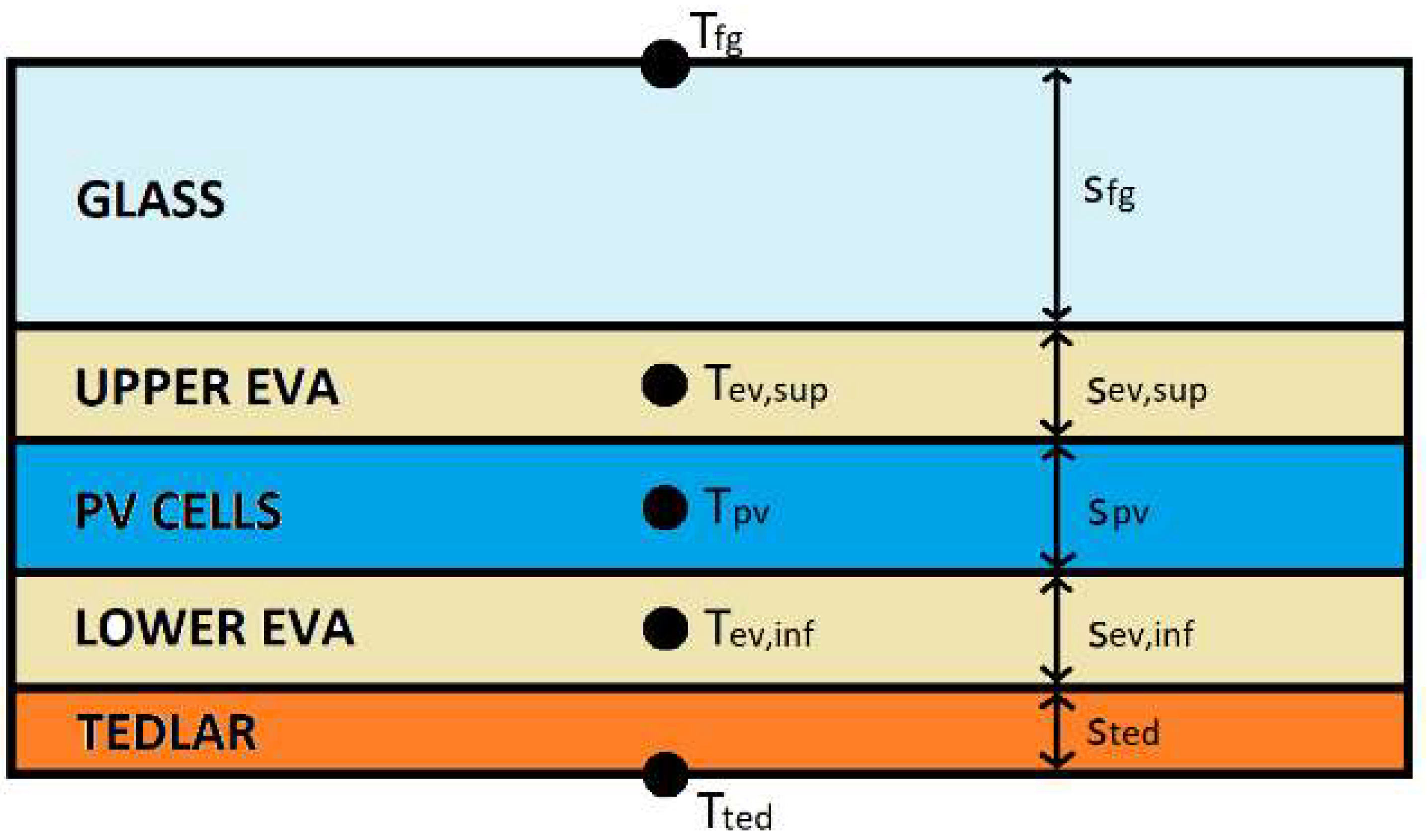
The aim of this study is to develop a simple calculation method to determine the temperature profile inside the PV panel and to provide information on heat dissipation. The code will be experimentally validated with data acquired at the laboratory of the University of Calabria. The model implements the energy balance equations of the layers also considering the capacitive terms. Developing a non-stationary model allows good results to be obtained even when atmospheric conditions change suddenly, for example, when a cloud passes. Furthermore, it allows the energy balance equations to be solved in a non-recursive manner, evaluating temperatures at the next moment. The model will later be used to derive information about the role played by each layer in heat dispersion. This aspect is important because it helps to choose the best strategy in case a cooling system is to be implemented.
The rest of the paper proceeds as follows; in
Section 2, the methodology to estimate the temperature profile is shown and the method to estimate the cloud cover is proposed. After providing information on the experimental setup, the model is validated in
Section 3. Useful results for understanding the heat loss in the panel will then be shown. Finally, in
Section 4, the results obtained are discussed.
3. Results
3.1. Validation of Sky Temperature Model
The equations are solved by determining the temperatures progressively at the next instant of time. The time interval considered for time discretization is 1 min in analogy with the acquisition of experimental data. The equations are structured in such a way that the system is solved in the “implicit mode” and the time interval does not generate problems of instability of the solution. The model used to determine the sky temperature has a considerable influence on the results. In order to determine the best model for estimating the sky temperature, the formulations usually used in the literature and the one proposed by this study were considered.
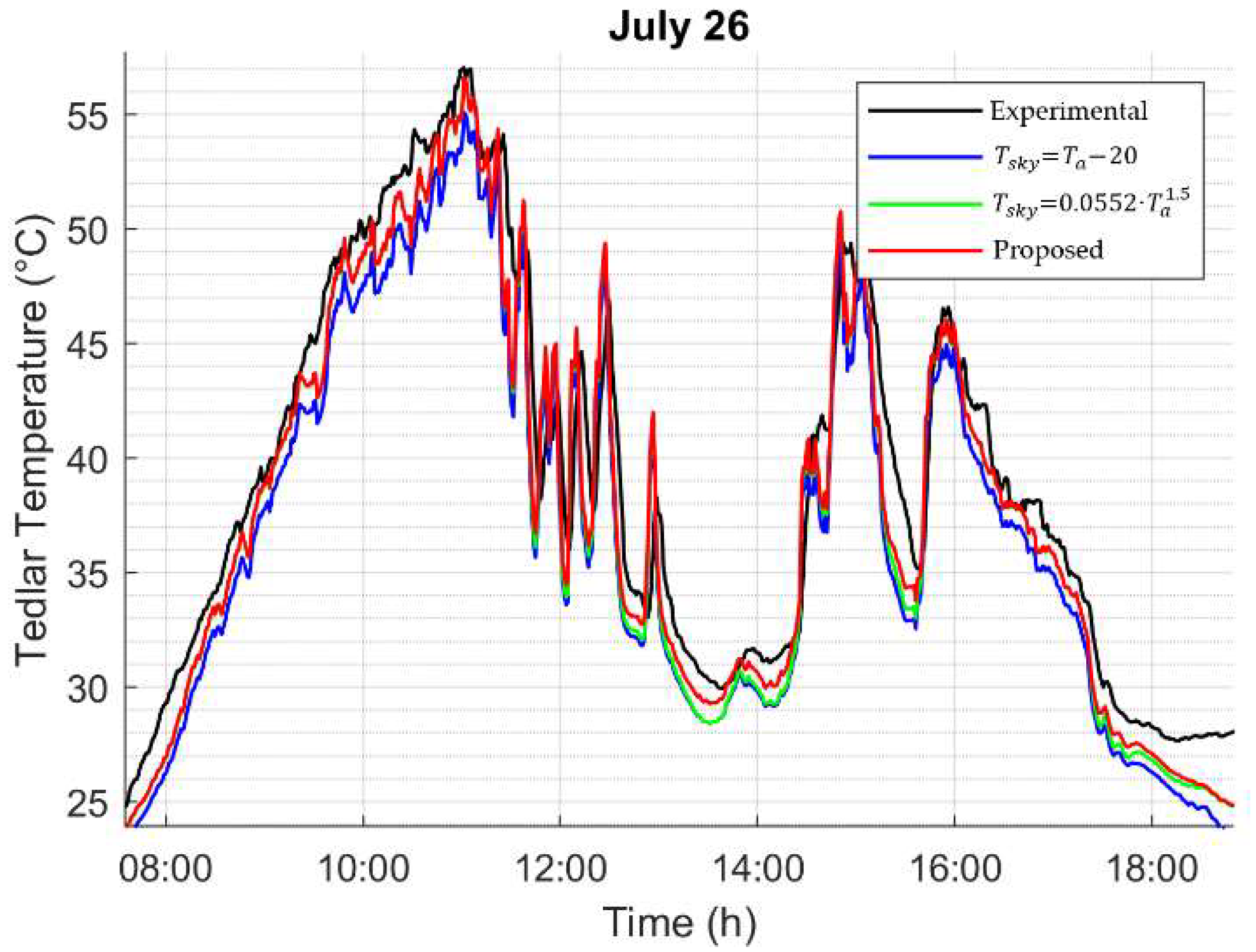
Figure 3 shows, as an example for 26 July, the comparison between the temperature values obtained for tedlar and the experimental values measured. The first model is based only on a reduction of 20 °C in the ambient temperature and approximates the results worse than the others. The day in question was cloudy at certain times in the afternoon. The Swinbank model and the proposed model show identical solutions in the morning hours, i.e., with clear skies. In the afternoon, due to the cloudiness of the sky, the panel temperature decreases. The proposed model, under these circumstances, provides a more accurate solution than the simplified model. It is able to recognize the cloudiness and a higher temperature is assigned to the sky, which reduces the radiative heat exchange with the PV panel.
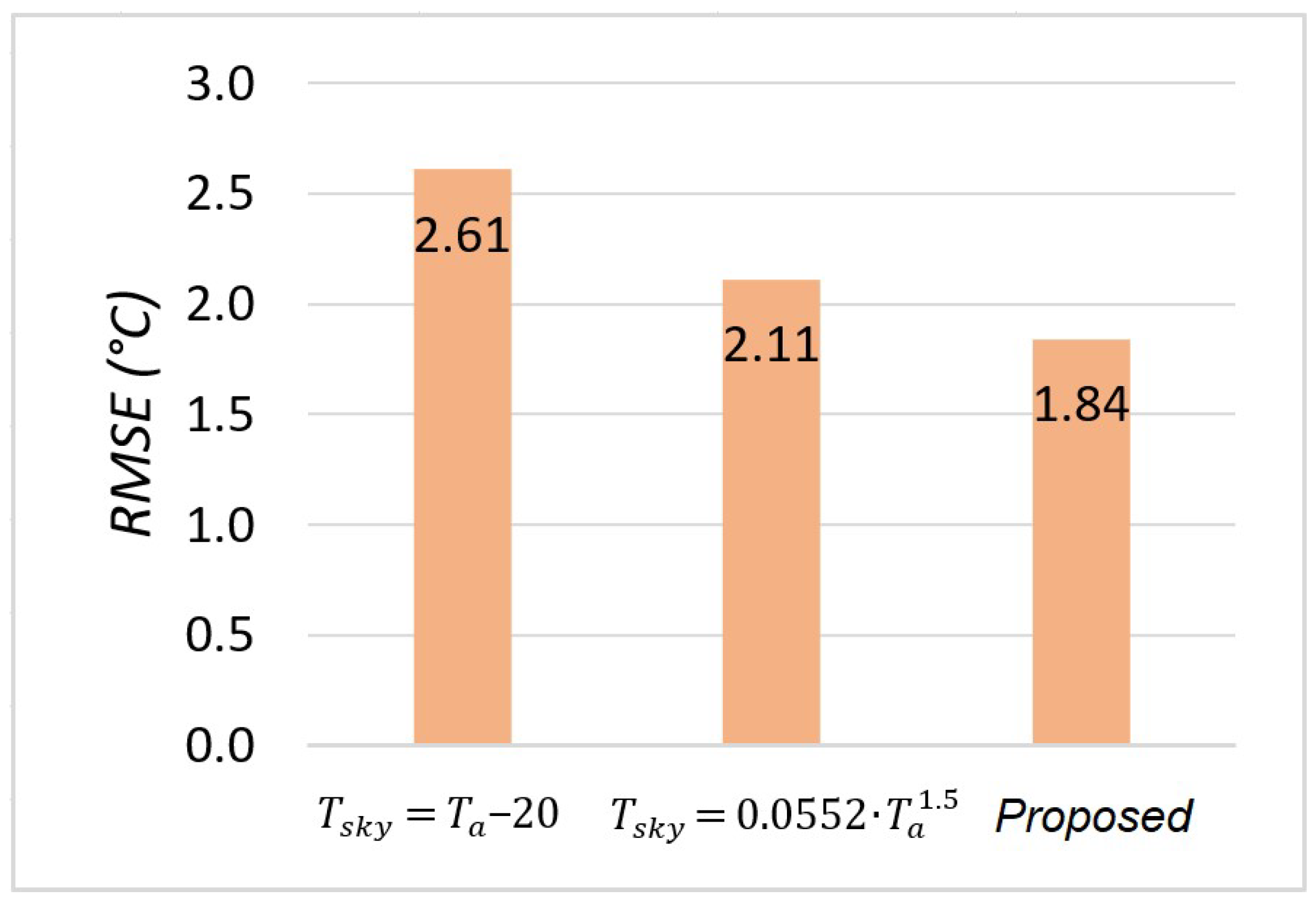
Figure 4 shows the root-mean-square error on the temperature obtained with reference to the measurements for the entire months of January and July. The proposed model allows the error to be reduced compared to the other methods usually used in the literature, obtaining an RMSE of 1.84 °C.
The model that will now be used to estimate the sky temperature will be the one proposed. Validation of the model will be conducted via winter and summer operation, with reference to both clear and cloudy days, with weak and strong winds.
3.2. Validation in Winter Conditions
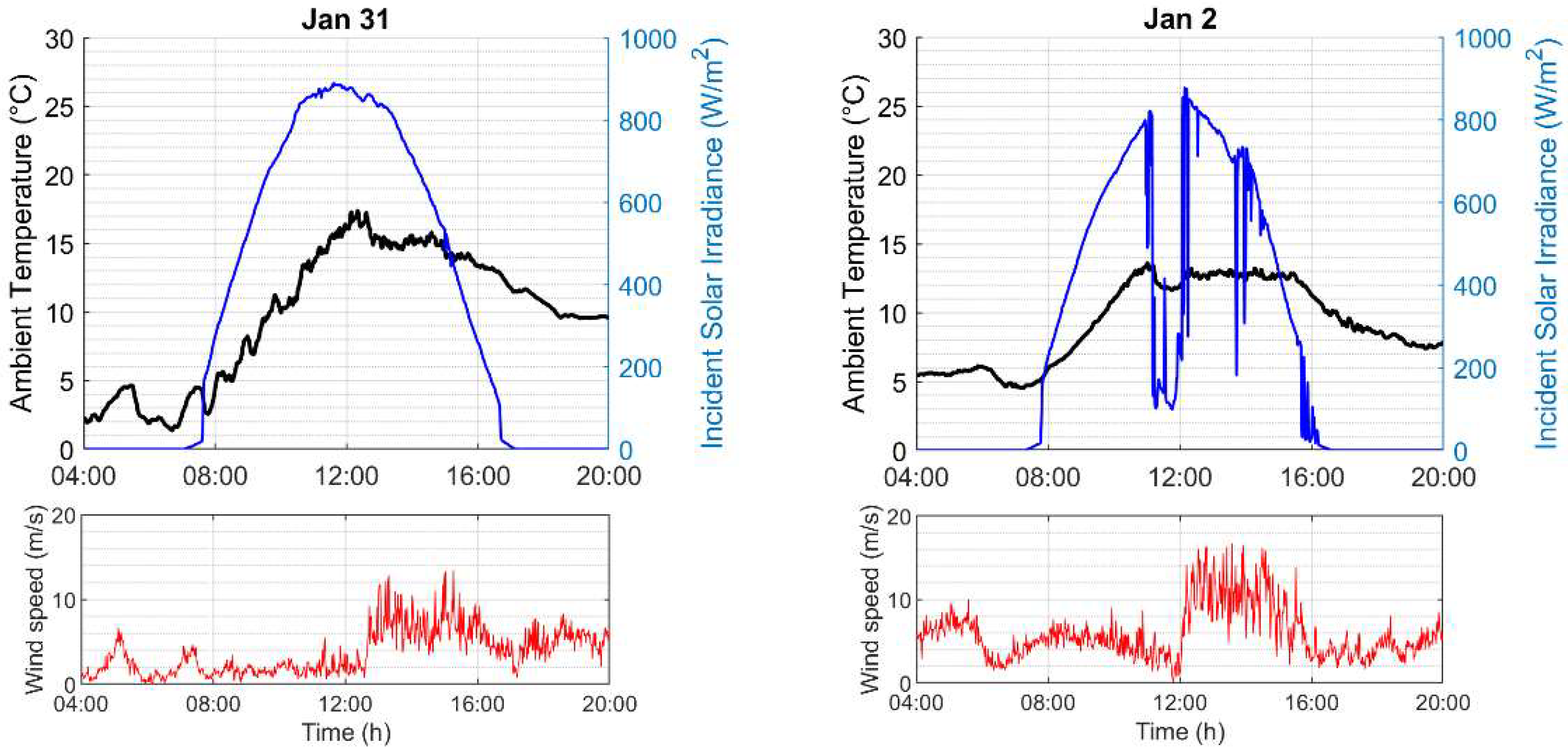
The results obtained for a clear winter day (31 January) and an overcast winter day (2 January) are analyzed to validate the model. The climatic conditions are shown in
Figure 5. The figure shows, on the left, the data for 31 January, which was a clear day, as can be seen from the solar radiation curve. On the right, the figure shows the climate data for 2 January, which was cloudy in the middle of the day and at certain times in the afternoon. During 31 January, the thermal variation was greatest; on 2 January the air temperature fluctuated between 5 and 14 °C and there was a reduction between 11:00 and 12:00, when the sky was cloudy. At the bottom, the figure shows the trends of wind speed, which was low in the morning for both days and then rose in the afternoon. These two days have been chosen because the wind was very variable and, therefore, it is possible to monitor the results with reference to flow conditions that can be laminar or turbulent.
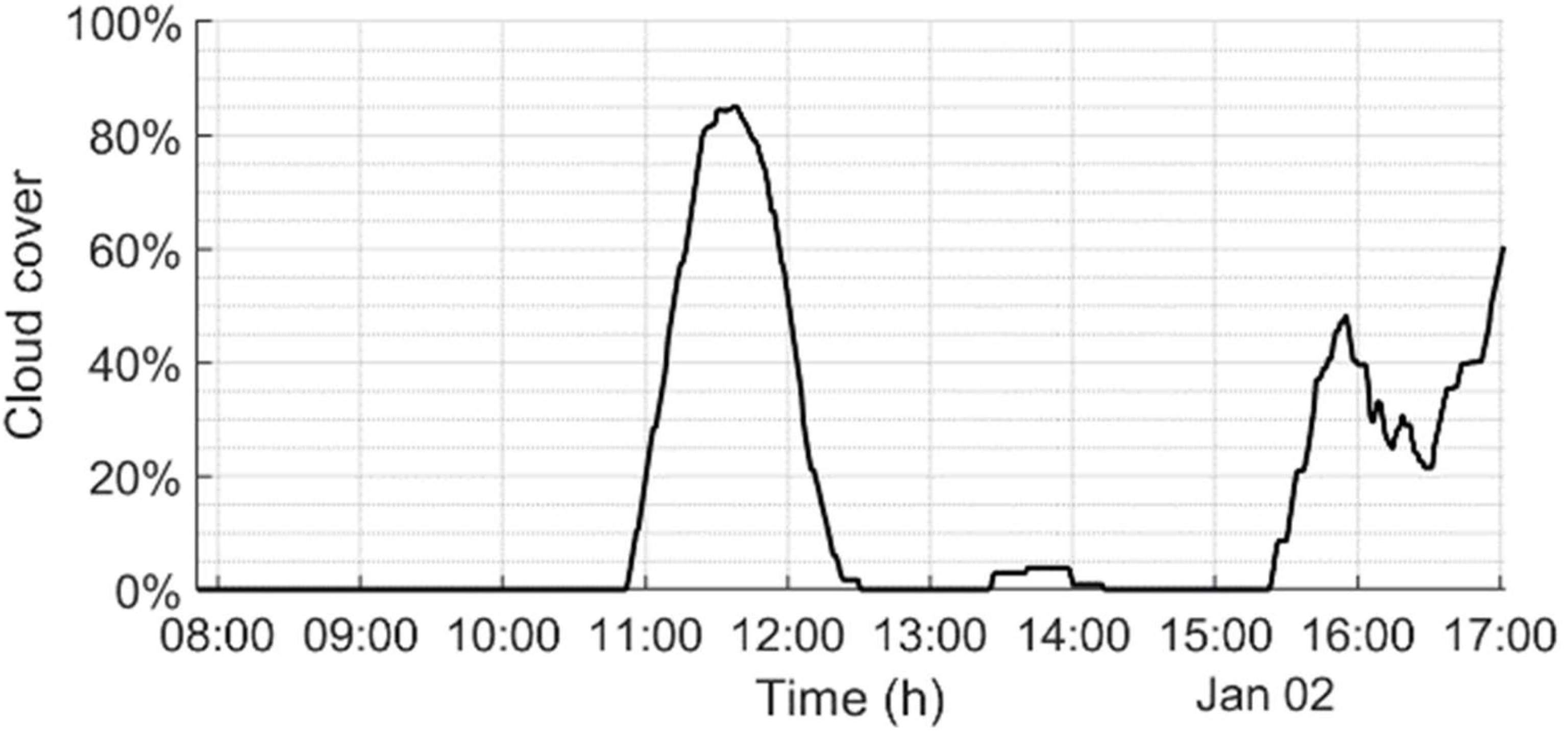
Therefore, the sky was cloudy between 11:00 and 12:00 on 2 January. We do not know if a small cloud covered only the solar disk or if the whole sky was cloudy. To avoid minor transient phenomena, the cloud cover is estimated by averaging it over one hour.
Figure 6 shows the percentage of cloud cover estimated with the proposed model. It can be noted that high cloud cover is observed in the central hours of the day, while at 14:00, the percentage of cloud cover is shown to be very low. In fact, the sky was probably not half-covered as it would appear from the reduction in solar irradiance, but a passing cloud may have covered only the solar disk. Thanks to the temporal averages, the cloud cover is about 85% in this first case, and it is less than 5% at 14:00. Before sunrise and after sunset, when the sun is not in the sky, the values are not of interest to us. However, in these cases, cloud cover is less accurately estimated based on the relative humidity value.
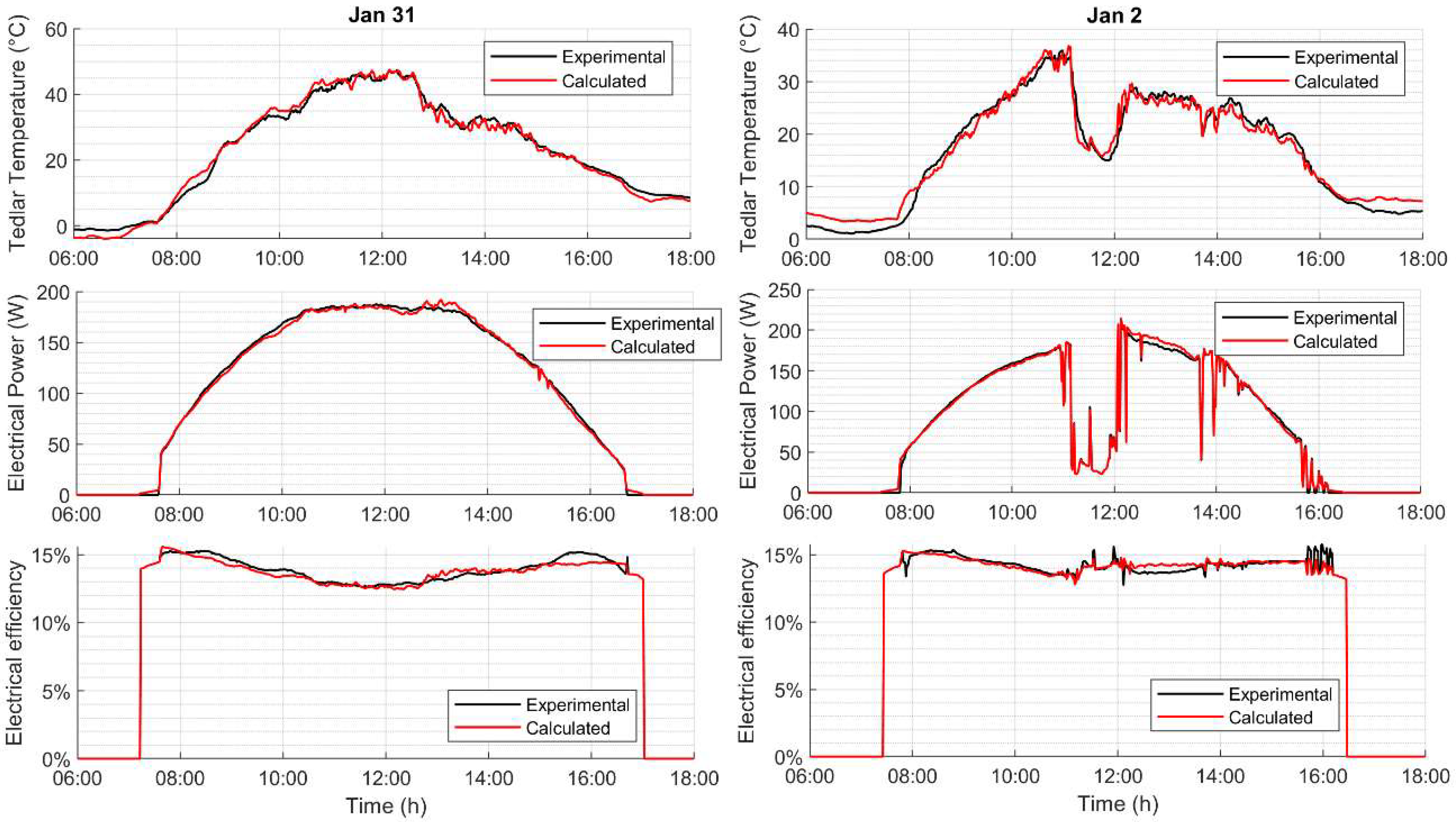
The values of tedlar temperature, electrical power, and electrical efficiency are shown in
Figure 7. The latter is calculated using Equation (6). The electrical power is obtained with the following equation:
The highest temperature value was reached on the clear day around noon and was 47.4 °C. From 12:30 onwards, there was a drastic drop in temperature, presumably due to the increase in the wind speed. In the early afternoon it was constant and around 30 °C. On the overcast day, on the other hand, the temperature started to decrease from 11:00 onwards as the radiation decreased. The values obtained from the mathematical model are very similar to those measured. The statistical parameters also confirm this qualitative consideration (
Table 2). In particular, the correlation coefficient CC is very high in both cases: over 0.99. The Nash–Sutcliffe efficiency (NSE) for the clear day is 0.989, which means that the accuracy of the model is excellent. It is slightly worse on the overcast day (0.964). The Mean Bias Error (MBE) is slightly negative, and this denotes a slight underestimation of the simulated data compared to the real ones. The root-mean-square error (RSME) is approximately 1.7 °C for the clear day and 1.8 °C for the overcast day.
With reference to the electrical power, the experimental values are well matched. It is only in the early afternoon that the estimated electrical power was slightly higher than the actual power for both days considered. This is due to the slight underestimation of the temperature in the same time slot. The statistical parameters confirm the good approximation of the model. The correlation index and the NSE are very high. The MBE is about half a Watt, and it is negative for the clear day and positive for the overcast day. The root-mean-square error is less than 3 W.
The electrical efficiency varies between 12 and 15% and this is confirmed by the experimental data. The statistical indices show, again, that the model adequately approximates the actual data. At 16:00 on 2nd January, the model shows a fluctuation in electrical efficiency. The experimental data do not agree with the prediction, as the actual oscillation is greater. These errors are usually present at dawn and dusk, when, in any case, electricity production is low.
3.3. Validation in Summer Conditions
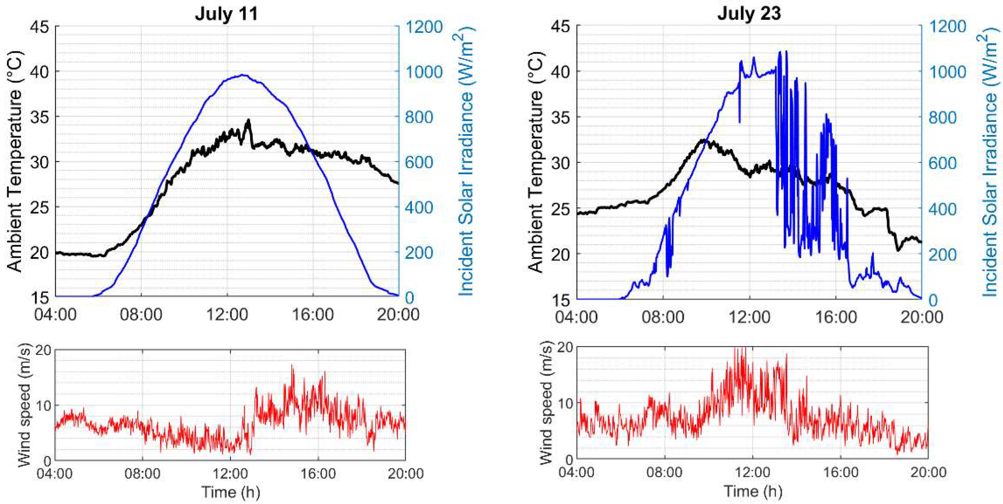
The summer validation is referred to 11 July and 23 July. Again, these represent a clear day and an overcast day. The global irradiance, ambient temperature and wind speed are shown in
Figure 8. During the clear day, the temperature varied between 20 and 35 °C, and decreased in the afternoon due to high wind speeds. On 23 July it reached a maximum of about 32.5 °C around 10:00 and decreased first due to high wind speeds and, in the afternoon, due to the absence of solar radiation. The days, again, were chosen with varying wind speeds throughout the day.
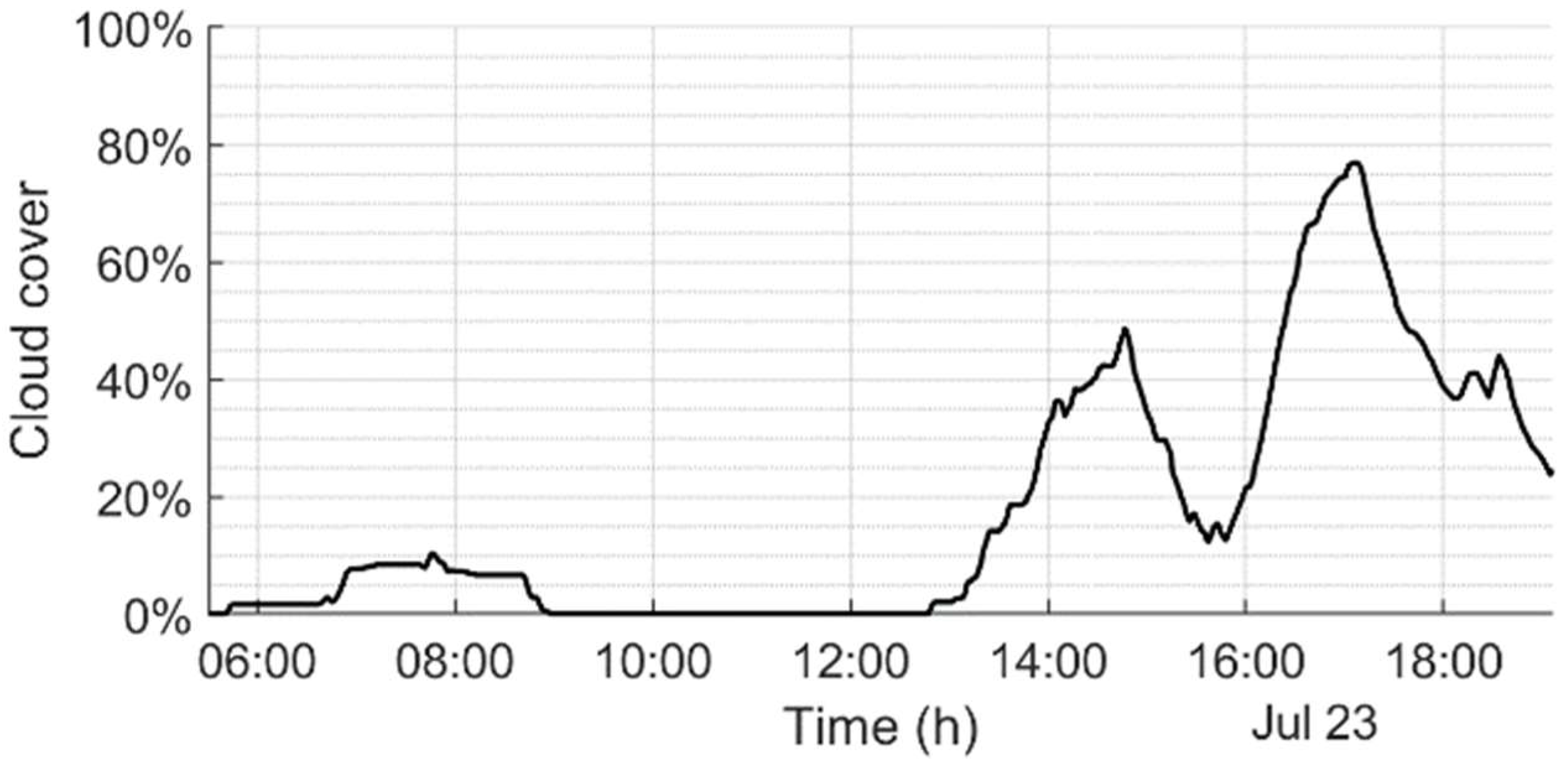
The percentage cloud cover estimated for 23 July is shown in
Figure 9. The sky is estimated to have been slightly overcast in the early morning hours (07:00–09:00), and two peaks of cloudiness are identified in the afternoon equal to 49 and 77%.
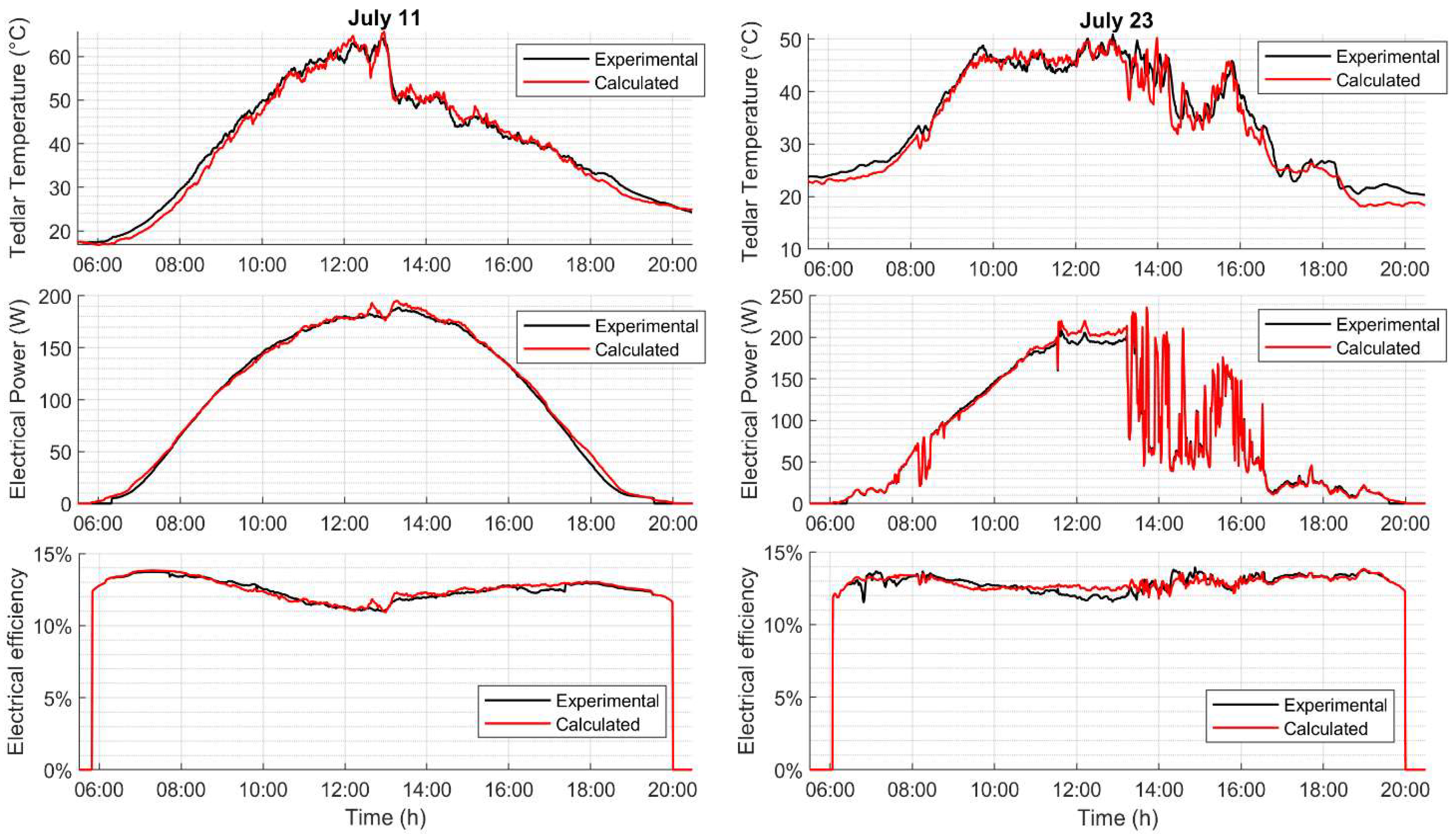
The tedlar temperatures are shown in
Figure 10. On 11 July, the maximum value reached was about 65 °C, well identified by the model. After 13:00, the temperature suddenly dropped to around 50 °C due to the turbulent flow generated by the high-velocity air. On 23 July, the panel cooled down slightly in the afternoon due to the reduction in solar irradiation. The model behaves adequately but, in this case, is less accurate than on the clear day. The correlation indexes are 0.996 for clear day and 0.983 for overcast day (
Table 3). The NSE also decreases in the case of overcast day, passing from 0.99 to 0.957. The MBE indicates that, in both cases, the data are slightly underestimated. The root-mean-square error is 1.4 °C for the clear day and 2.25 °C for the overcast day.
The model predicts electrical output quite well, especially when irradiance is highly variable. For the clear day, the MBE is +1.7 W and RMSE is 3.4 W. CC and NSE are, instead, excellent. The model slightly overestimates electricity production at noon. With reference to the electrical efficiency, the NSE is about 0.98. For the overcast day, on the other hand, the MBE is about the same as in the previous case, but with a higher RMSE. Again, there is an overestimation at midday, although the temperature is well identified at this time.
3.4. Temperature Profile along Panel and Influence on Heat Dispersion
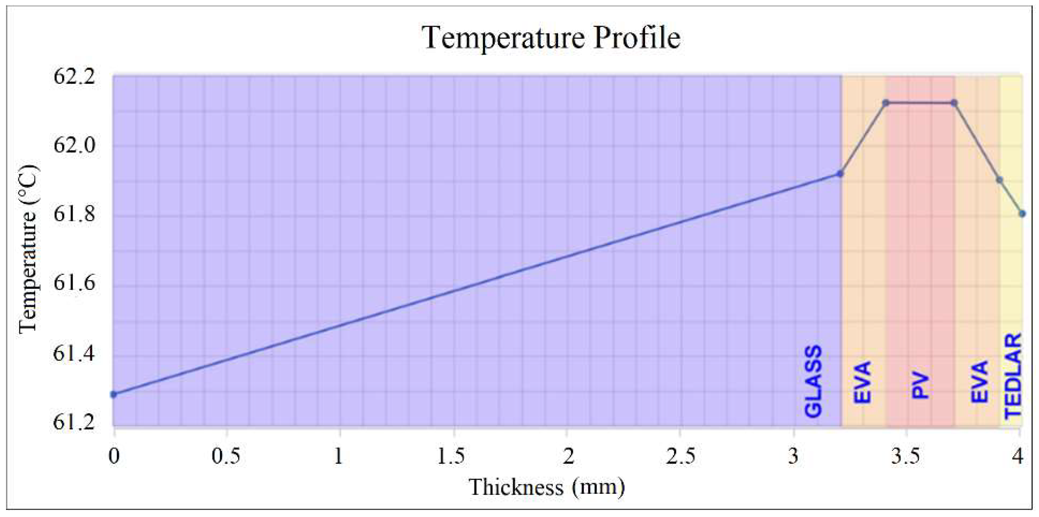
Figure 11 shows the temperature profile within the entire panel assessed by the model at 12:00 on 11 July. The outside air temperature is 34.6 °C, the global irradiance measured on the panel plane is 978 W/m
2 and the wind speed is 7.1 m/s.
Thanks to the model, it is possible to calculate the temperatures of the nodes for which the balance equations were written. It is possible, moreover, to identify the temperatures at the layer interfaces using a simple electrical analogy.
Figure 11 shows that temperature is almost uniform within the panel, oscillating between 61.3 and 62.1 °C. The hottest component is the PV layer, while the coldest one is the outer surface of the glass, despite being directly exposed to sunlight. The temperatures on the two sides of the panel are different. It may seem anomalous that the temperature in the tedlar surface is higher than that in the glass surface. Tedlar, in fact, is a thermal insulator and it was expected that the temperature of its outer face could be close to the temperature of the air (or at least lower than the temperature of the face of the glass, which is also directly exposed to the sun’s rays).
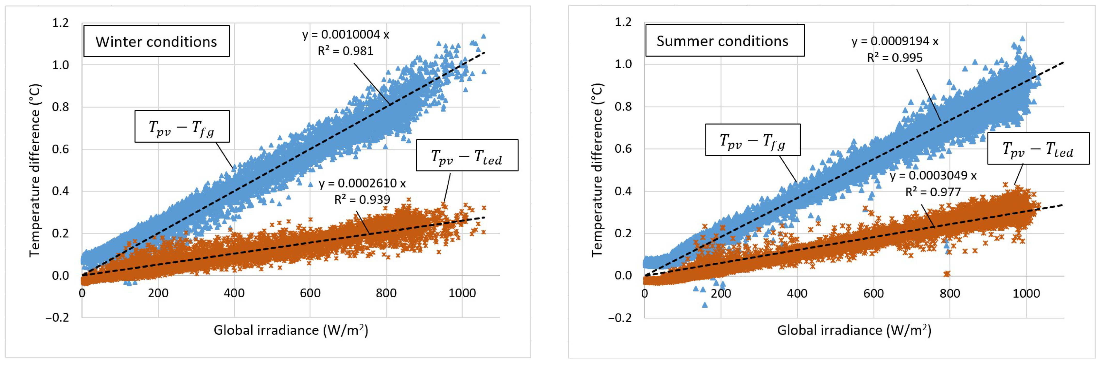
The graphs in
Figure 12 correlate the temperature difference between the PV layer and both the surfaces of the front glass and tedlar with the irradiation values. The figure shows that the internal temperature gradients are linearly proportional to the irradiance
incident on the panel. The evidence found on 11 July at noon (tedlar temperature higher than glass temperature) is confirmed under all operating conditions.
In fact, blue dots in the figure are almost always placed higher than the orange dots. Only for a few points, in low irradiation conditions, is there an overlap between the two areas. In these few cases it may result in the temperature of the glass being higher than the temperature of the tedlar.
The figure distinguishes between winter and summer conditions. With reference to winter conditions, the temperature difference is linearly linked with global radiance by means of the correlation with . The temperature difference, instead, between the PV layer and the tedlar surface is linked with global irradiance by means of the equation with . On average, therefore, the temperature deviation with tedlar is four times lower than with the front glass surface. In summer operating conditions, the graph is similar to the previous one and the linear proportionality with the global irradiance is confirmed. The interpolating equations change slightly. With reference to the temperature difference between the PV layer and the front glass, the equation is with ; the temperature difference with the tedlar, on the other hand, has a correlation of with . The equations are quite similar between the winter and summer case, but in the latter case it turns out that the temperature difference with the tedlar is about three times smaller than the temperature difference with the front glass.
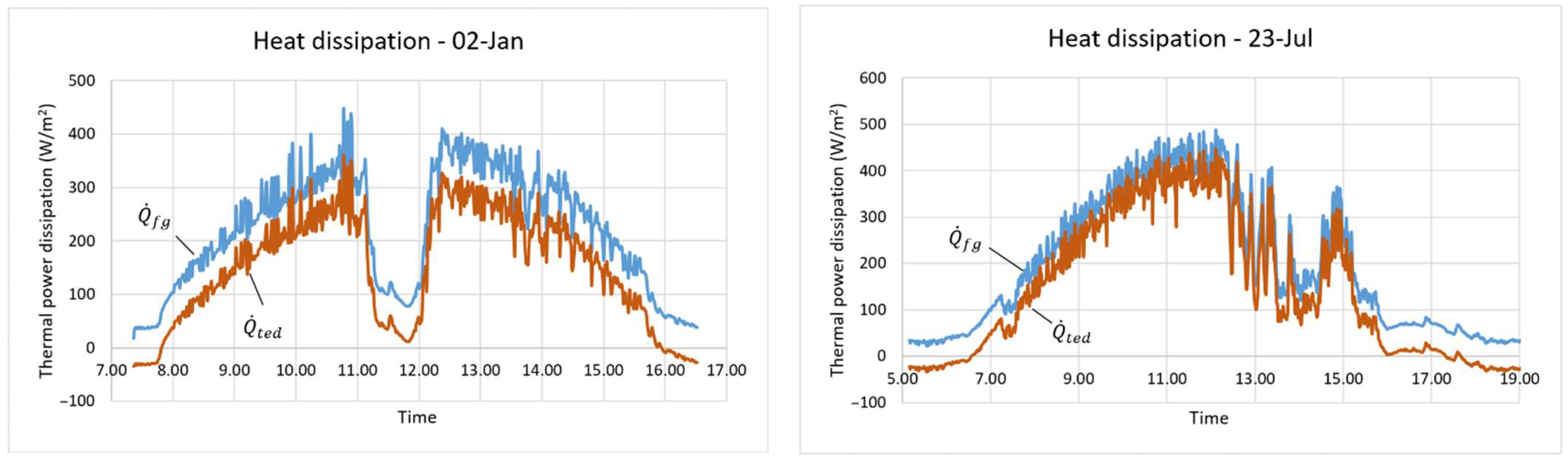
The glass surface is therefore cooler than the back of the panel. However, this does not mean that it dissipates less heat by convection and radiation. On the contrary, the graphs in
Figure 13 show that it is the cooler of the two surfaces (the front glass) and dissipates the most heat, under all conditions. The figure shows the trends of
and
indicating the thermal power lost to the outside by convection and radiation from the front glass and tedlar, respectively. The negative values of
, recorded in the morning and evening, represent the moments when the air temperature was higher than the surface; here, the back of the panel is heated by the air, by radiation, and by the environment. Heat loss is greatly influenced by wind speed. In fact, the fluctuating trends are caused by the varying wind intensity.
is always higher than
by about 50–100 W/m
2. In the summer period, the behavior is similar; however, the differences between the two curves are slightly smaller.
4. Discussion
The model allows temperature results to be estimated with simple methodology and good accuracy. The overall RMSE obtained for temperature is 1.84 °C. This result is lower than that of other works in the literature, such as Mavromatakis et al. [
19] (∼2.1–2.2 °C) and Mattei et al. [
21] (2.24 °C). The error is greater when compared to more complex methods. For example, Bevilacqua et al. [
30] and Aly et al. [
23] obtained an RMSE of 1.37 °C and between 0.94 and 1.35 °C respectively by using numerous nodes to discretize the PV panel. The methodology presented in this paper for estimating cloud cover has given very good results. It is based on the comparison between the measured irradiance and the theoretical irradiance under clear sky conditions. It has made it possible to reduce the RMSE temperature from 2.11 to 1.84 °C.
The study provided a simple method for estimating the performance of a PV panel. In addition, the proposed new sky temperature relationship can be used for research purposes in the photovoltaic and other fields.
The temperature profile shows that the highest temperature is reached by the PV cell. However, the temperature remains quite homogeneous within the entire panel: the maximum gradient is about 1 °C. This characteristic allows an easier thermal dispersion of the absorbed heat. The temperature of the glass is cooler than the temperature of the back of the panel. In addition, the upper surface dissipates more heat power than the lower surface. The study, therefore, suggests that any cooling system should be applied on the back side to increase heat exchange.
5. Conclusions
The paper presented a simple one-dimensional transient model for estimating the temperature profile in a PV panel and the electrical power generated. The results were experimentally validated using a PV panel and the appropriate sensors placed on the 45/C building of the DIMEG at University of Calabria. The validation was carried out under both clear and overcast conditions, for both winter and summer days. In order to simulate overcast days, a methodology is proposed and validated for recognizing cloud cover. This information is necessary as it has a significant influence on the radiative heat exchange.
The model is able to predict the temperature of the back of the panel with an RMSE of about 1.5–2.0°. The RMSE on the estimation of the delivered electrical power is 2.5–4.3 W. The RMSE on the electrical conversion efficiency is 0.25–0.75%. In both summer and winter periods, the MBE on the temperature estimation is negative, with values ranging between −1.0 °C and −0.5 °C. This means that the model returns slightly lower values than the real ones. The limitation of the present study is that the problem is considered one-dimensional. The temperature obtained is assumed homogeneous for the faces. This methodology does not allow for the evaluation of edge effects and does not consider the nonuniformity of the photovoltaic layer. However, the errors are acceptable because they are often lower than errors obtained through other scientific studies using more complex models.
The study found that the back of the panel reaches high temperatures and dissipates less thermal power than the front face. Facilitating cooling of the back face could be a useful solution to keep cell temperatures lower and improve panel efficiency. For this role, an effective solution is spray cooling, which involves spraying water mist droplets on the surface and waiting for them to evaporate by absorbing the latent heat of evaporation. The study shows that this solution should be adopted on the back face instead of the front face, and a study of its effectiveness represents a possible future development for this work.


 ,
, 


