Deep Learning Prediction for Rotational Speed of Turbine in Oscillating Water Column-Type Wave Energy Converter

Abstract

This study uses deep learning algorithms to predict the rotational speed of the turbine generator in an oscillating water column-type wave energy converter (OWC-WEC). The effective control and operation of OWC-WECs remain a challenge due to the variation in the input wave energy and the significantly high peak-to-average power ratio. Therefore, the rated power control of OWC-WECs is essential for increasing the operating time and power output. The existing rated power control method is based on the instantaneous rotational speed of the turbine generator. However, due to physical limitations, such as the valve operating time, a more refined rated power control method is required. Therefore, we propose a method that applies a deep learning algorithm. Our method predicts the instantaneous rotational speed of the turbine generator and the rated power control is performed based on the prediction. This enables precise control through the operation of the high-speed safety valve before the energy input exceeds the rated value. The prediction performances for various algorithms, such as a multi-layer perceptron (MLP), recurrent neural network (RNN), long short-term memory (LSTM), and convolutional neural network (CNN), are compared. In addition, the prediction performance of each algorithm as a function of the input datasets is investigated using various error evaluation methods. For the training datasets, the operation data from an OWC-WEC west of Jeju in South Korea is used. The analysis demonstrates that LSTM exhibits the most accurate prediction of the instantaneous rotational speed of a turbine generator and CNN has visible advantages when the data correlation is low.

1. Introduction

As the global energy demand increases with an increasing population, renewable energy systems are regarded as an indispensable alternative energy source in terms of technological maturation and carbon footprint reduction [1]. A number of studies have reported the introduction of power grids that incorporate renewable energy sources [2,3,4,5]. In this context, wave energy will play a key role as an energy source, as it has the potential for an annual energy generation of 29,500 TWh [6,7,8].

The oscillating water column (OWC)-type wave energy converter (OWC-WEC) with air turbines is one of the most state-of-the-art concepts for utilizing wave energy [9] and is regarded as the most reliable method for doing so. The air turbine driving the generator is an essential component of the power plant, where the pneumatic energy from the waves is converted into useful electrical energy. The turbines for wave energy are subject to more challenging conditions than conventional turbines. The air flow velocity is irregular and varies significantly according to the oceanic conditions, and the operational direction is reversed twice in the wave cycle. OWC prototypes have been in operation in several countries (e.g., the Pico wave power plant in Portugal [10], LIMPET wave power plant in Scotland [11], Mutriku wave power plant in Spain [12], NIOT power plant in India [13], OE Buoy in Ireland [14], and renewable energy power plant in Jeju Island in South Korea [9]).

The control strategy of the OWC-WEC can be classified into two categories. One is utilizing the maximum power point control [15,16,17] to obtain the maximum power according to the input energy, and the other is the peak shaving control [18,19] to limit the energy input to below the system rated value. In a renewable energy system, because the energy input is highly variable, controlling the maximum power according to the input energy is essential. However, due to the nature of highly variable wave energy with a large peak-to-average power ratio, the operating time and cumulative power generation will be reduced without adequate peak shaving control [18,19]. In [18], using a relief valve and a high-speed stop valve based on an electrical test device and hardware in the loop testing method, a comparative study on rated power control performance was conducted. In another study [19], the performance of the control algorithm using a high-speed stop valve was compared, and an improved performance was achieved through a monotonous valve angle change using an instantaneous rotational speed. This demonstrates that a high-speed stop valve is suitable for controlling energy input above the OWC-WEC rated value, but a more elaborate control method is needed to overcome the volatile wave energy input [18]. The current rated power control method using instantaneous rotational speed requires an energy input, which has already been introduced to the system. Thus, it is difficult to control when there is an instantaneous input from a large energy spike. In addition, even when the high-speed safety valve is in operation, an operating time is required. Therefore, a faster control method that overcomes this limitation is needed.

An artificial neural network (ANN) is a widely used modeling and prediction tool that offers an alternative method for solving complex problems. ANNs can learn from training using datasets and, with the necessary training, they can quickly perform predictions and generalizations [20]. Deep learning technology, a subset of AI, is used to obtain a more stable and accurate system performance and has proven to be an excellent tool for tackling various energy application problems, including overcoming the volatile nature of renewable energy [21,22,23,24,25]. For example, a method for tracking the hourly state of sunshine for solar power generation has been developed [21], and a study [22] that analyzed the influencing factors for solar irradiance forecasting was conducted. For applications in wind power, there has been research on the improvement of wind speed prediction performance [23,24] as well as a study on wind speed prediction on a daily, weekly, and monthly basis [25]. In addition, there has been a study on the operation of an energy storage system to increase economic efficiency by predicting the power generation output of a renewable energy system [26]. As AI-based prediction techniques have been adopted in various renewable energy fields, the characteristics of even volatile wave energy are expected to be controlled in a more precise manner if a control method based on AI technology is employed.

In this study, the instantaneous rotational speed of the OWC-WEC is predicted by applying a deep learning algorithm that is suitable for nonlinear control among the abovementioned AI technologies. The proposed method predicts the instantaneous rotational speed of a turbine system after 2 s, considering the valve operating time. If this prediction method is adopted for rated control, the valve can be operated before the energy input above the rated value is introduced to the plant, thus enabling more control. To predict the instantaneous rotational speed of the OWC-WEC, various deep learning algorithms, such as multi-layer perceptrons (MLPs) [27], recurrent neural networks (RNNs) [28], long short-term memory (LSTM) [29], and convolutional neural networks (CNNs) [30], are applied to the same input conditions and the prediction performance is compared between these different algorithms. In addition, the dataset composition for the prediction of the instantaneous rotational speed is defined through the performance analysis of the deep learning algorithm, according to the composition of the training datasets. As for the datasets used in this study, the operation data of the OWC-WEC located in a real wave power plant test site in western Jeju were used to verify the performance of each algorithm.

2. Conventional Method for OWC-WECs

2.1. Load Control Algorithm (Maximum Power Point Tracking)

Control methods to maximize the power generated by OWC-WECs have been investigated in several studies [15,16,17]. These studies experimentally examined maximum power control methods by combining a turbine and a generator. Based on the instantaneous rotational speed, the electrical power for obtaining the maximum power is calculated as [31]

$$P_{\mathrm{e}}^{\ast }=\left({\eta }_{\mathrm{T}.\max }\ast C_{\mathrm{A}.\mathrm{opt}}\ast \beta \ast \left[1+\frac{1}{{\varnothing }_{\mathrm{opt}}^2}\right]\ast r_{\mathrm{t}}^3\ast {\varnothing }_{\mathrm{opt}}^3\right)\ast {\omega }_{\mathrm{m},}^3$$

(1)

where ${\eta }_{\mathrm{T}.\max }$ represents the maximum efficiency of the turbine system, and $C_{\mathrm{A}.\mathrm{opt}}$ and ${\varnothing }_{\mathrm{opt}}^2$ are the input coefficient and flow coefficient that maximize the efficiency of the turbine system, respectively.

However, considering the effect of the inertia of the rotating mass of the turbine and the hydrodynamic power take-off (PTO) damping of the WEC in its actual operation, the electrical power required to generate the maximum power output of the turbine system is calculated by

$$P_{\mathrm{e}}^{\ast }=k_a\ast {\omega }_{\mathrm{m}}^b,$$

(2)

Equation (2) is used to maximize the time-averaged power output based on the instantaneous rotational speed of the turbine generator. However, in offshore conditions with large amounts of wave energy, the electrical hardware may not be able to apply a specified electromagnetic torque due to the rated capacity limit. As a result, the rotational speed of the turbine increases beyond the limit. To solve this problem, studies have been conducted to investigate how to control the energy input from reaching above the rated power of an OWC-WEC [18,19].

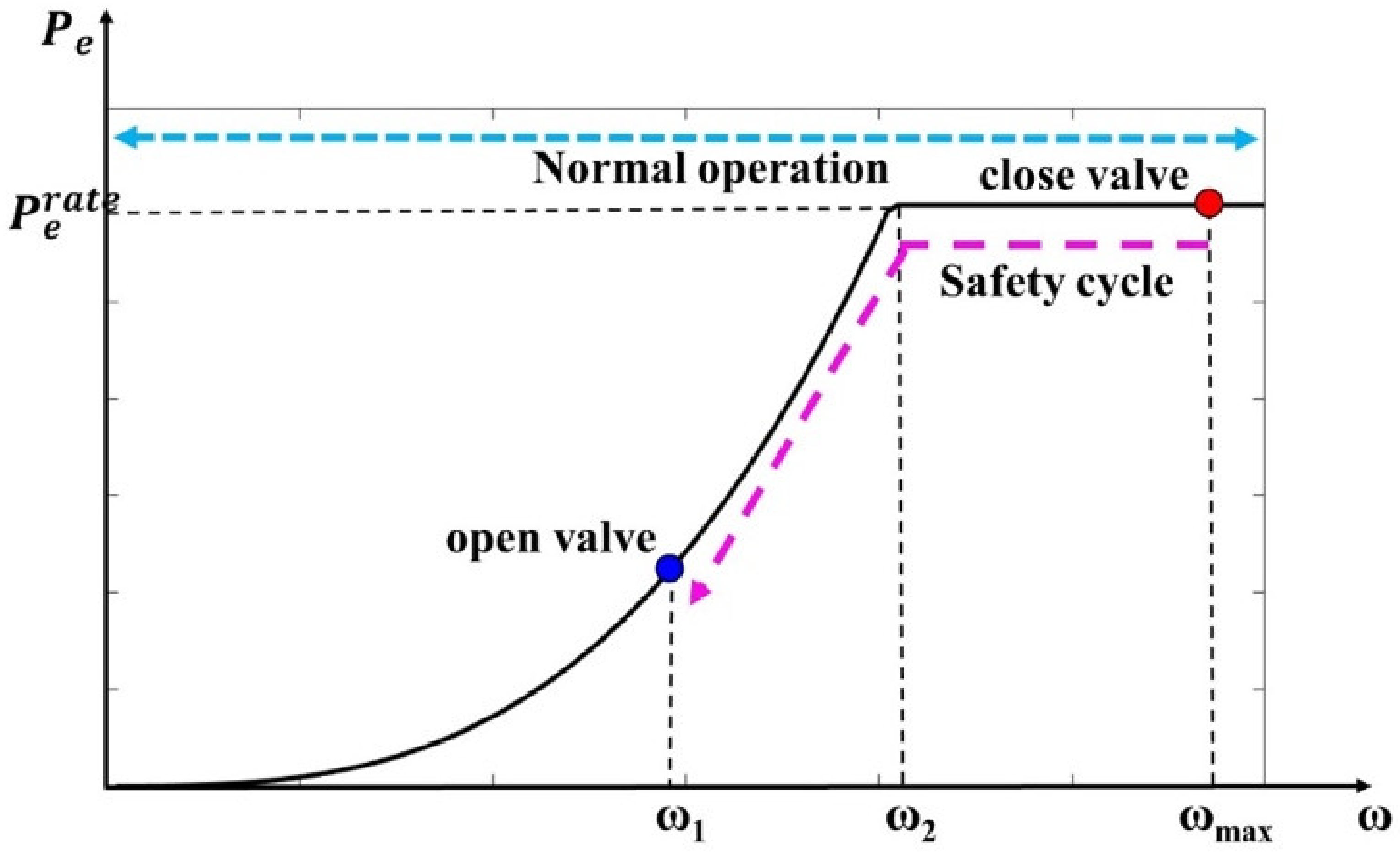
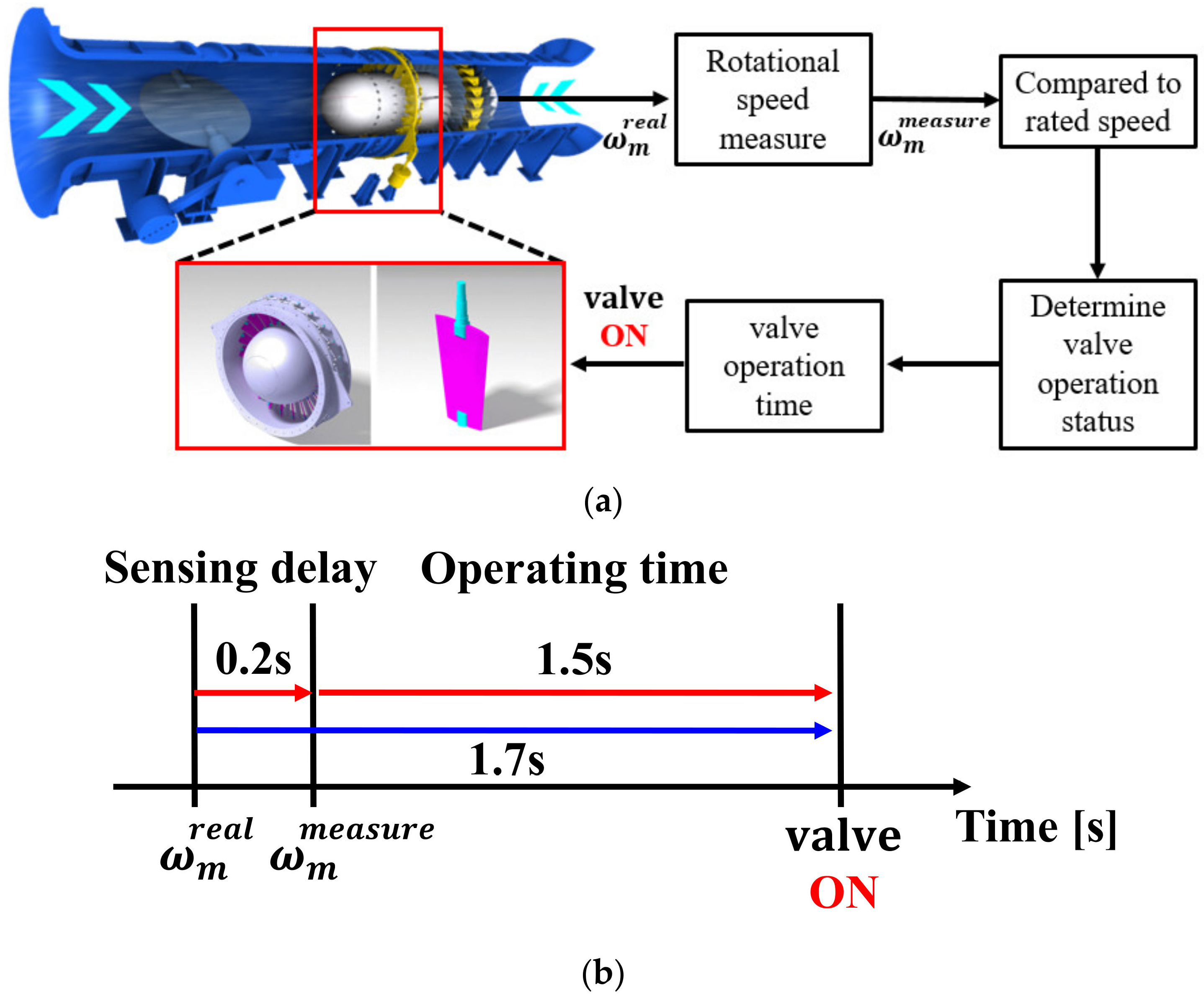
2.2. Rated Control Algorithm (Peak Shaving)

As shown in Figure 1, an OWC-WEC controls the load according to the instantaneous rotational speed. In normal operation mode, the maximum power control is performed via an electromagnetic torque that is applied according to the instantaneous rotational speed of the turbine generator, and the high-speed safety valve limits the energy input when the instantaneous rotational speed of the turbine generator exceeds the maximum value.

When the instantaneous rotational speed of the turbine generator is between two user-defined values, the maximum power control is performed using (2). When the instantaneous rotational speed of the turbine generator is in between the upper user-defined value and the maximum, the power control is performed using the rated power via

$$P_{\mathrm{e}}^{\ast }=P_{\mathrm{e}}^{\mathrm{rate}},$$

(3)

where $P_{\mathrm{e}}^{\ast }$, $P_{\mathrm{e}}^{\mathrm{rate}}$ represent the reference control power and rated power, respectively. In addition, when the speed is higher than the maximum value, it operates in safe mode by closing the high-speed safety valve, after which the instantaneous rotational speed of the turbine generator decreases. When the instantaneous rotational speed falls below the lower user-defined value, the valve is opened again.

The energy peak can be controlled using the abovementioned method, but energy input above the rated value may still be randomly introduced due to the highly volatile nature of wave energy. It is difficult to predict when an energy input above the rated value will be randomly introduced to the system because the peak-to-average power ratio is greater than 10. The conventional rated power control method is based on the current instantaneous rotational speed of the turbine generator. However, the current instantaneous rotational speed is measured after the energy input, making precise rated control difficult. In addition, there is a valve operating time and this also hinders precise rated control. In light of this, a precise rated control method that can address the limitations of the conventional rated control is required.

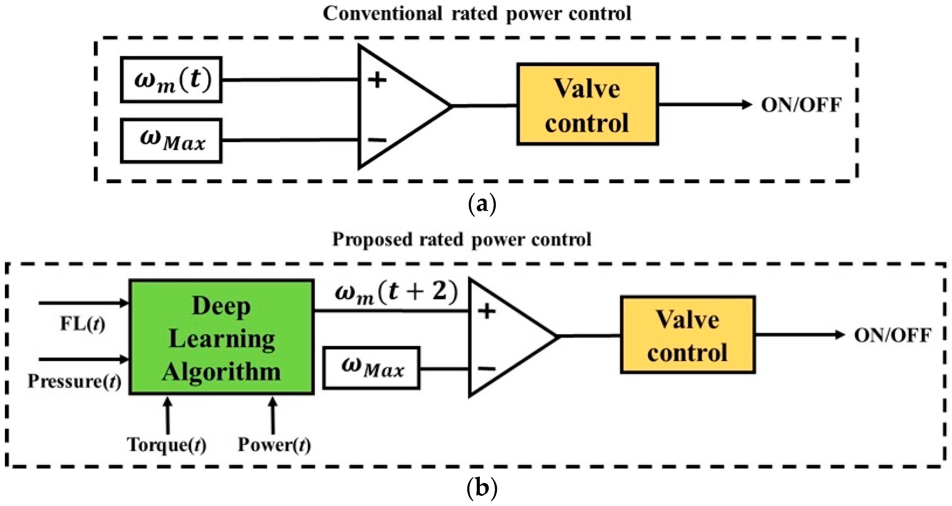
3. Application of Deep Learning Algorithm for Precise Rated Control for OWC-WECs

3.1. Data-Based Power Variation Prediction Technology

Deep learning algorithms have been employed in various ways for power output prediction in the energy sector [32]. Deep learning algorithms use data affecting power generation as training datasets. With this information, they construct a suitable ANN for the accurate prediction of power output. Various deep learning algorithms have already been applied to the prediction of power generation. Renewable energy systems experience large fluctuations in the energy that they receive, making power generation predictions difficult. Therefore, a technique for predicting power output using a deep learning algorithm is needed [32].

OWC-WECs are difficult to control because highly unpredictable and volatile wave energy is used as the input. In particular, the peak-to-average power ratio is more than 10, which necessitates an appropriate control method [18,19]. In conventional methods, a high-speed safety valve is used to prevent the energy input from reaching above the rated value [18], but the precise control of the input energy with volatile instantaneous changes still remains a challenge. To overcome this difficulty, the rated capacity of the PTO system can be increased, but this would lead to a sharp decrease in efficiency and an increase in the cost of generating a small amount of energy. Therefore, if a deep learning algorithm is applied to predict the power generation and the valve can be operated based on that prediction, it will be possible to overcome the limitations of the conventional rated control method.

The conventional rated power control algorithm changes the angle of the valve by comparing the turbine’s current rotational speed to the rated rotational speed [18,19]. Figure 2a shows the valve operation mechanism of the rated control algorithm. However, as shown in Figure 2b, due to the sensor measurement delay and valve operating time, the response of the valve control is a delayed when using the turbine’s rotational speed. Therefore, the valve control proposed in this study predicts the turbine’s rotational speed using the data of its state 2 s after the present time by applying a deep learning algorithm. In this way, it controls the angle of the valve by comparing the predicted rotational speed and the rated rotational speed. Figure 3 shows a block diagram of the conventional and proposed algorithms. To accurately predict the turbine’s rotational speed, the prediction performances of various deep learning algorithms were compared. Each deep learning algorithm is described in the next section.

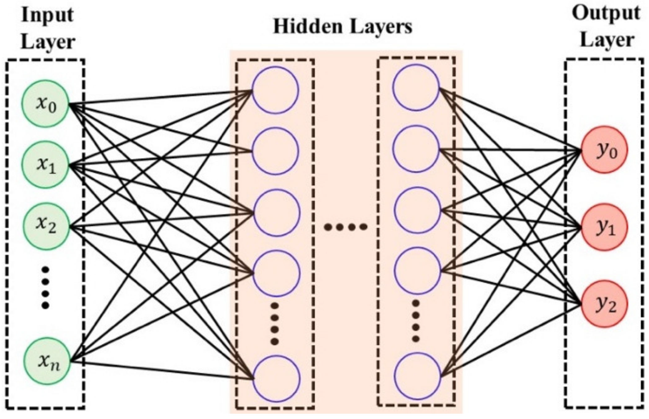
3.2. Classification of Deep Learning Algorithms for Prediction of Turbine Rotational Speed

• Multi-Layer Perceptron (MLP)

There are various types of neural network architectures [27,28,29,30] in deep learning algorithms, but the simplest and most original ANNs are MLPs. Figure 4 shows a block diagram of the architecture of an MLP. In general, an MLP consists of three layers: an input layer; a hidden layer; and an output layer. An MLP neural network has one or more hidden layers and, in deep learning algorithms, the network is typically composed of three or more hidden layers. These multiple layers are fully connected (i.e., the neurons in the upper layer and those in the lower layer are fully connected).

The principle of MLPs is to compute the result using the weight and activation function of the input data, and to repeat this computation until the output layer is reached. All layers of an MLP are arranged in a feedforward network and no feedback connections are allowed. The MLP algorithm calculates the weights and biases of each layer to perform the training. Using the input data, the k-th output (y_k) can be represented by [27]

$$y_k=\max (0,{\sum }_{i=1}^n\left({\omega }_i{x}_i+b_k\right)),$$

(4)

The calculated results are compared to the actual values, backpropagation is used to reduce errors, and the model is continuously updated. A gradient descent is used to update the weights to reduce the errors. Using the gradient value for the current weight, the updated weight can be calculated as

$${\mathsf{\omega }}^{t+1}={\mathsf{\omega }}^t-\frac{d\left(error\right)}{d\omega },$$

(5)

For the activation function, the Rectified Linear Unit (ReLU) function is used to solve the problem of loss in the error gradient due to the nature of deep learning algorithms composed of multiple layers. The ReLU is represented as

$$\mathrm{ReLU}\left(x\right)=\max (x,0).$$

(6)

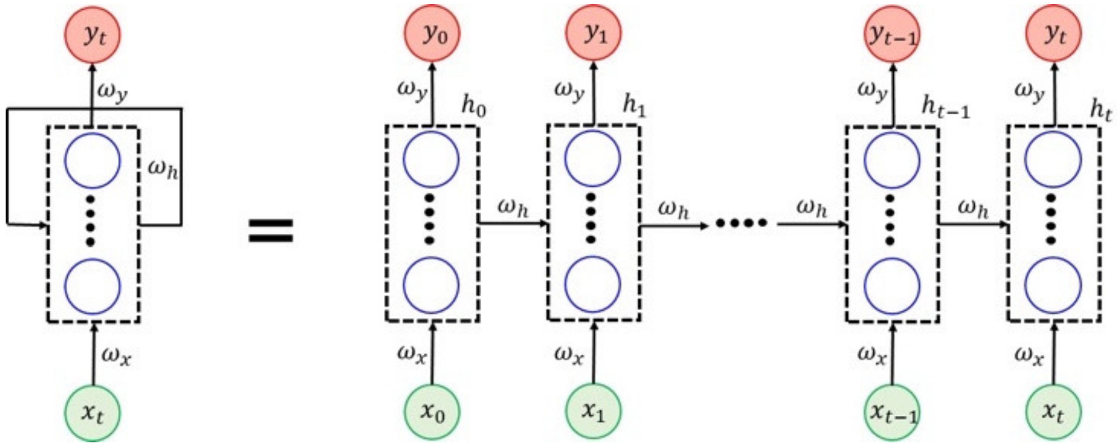
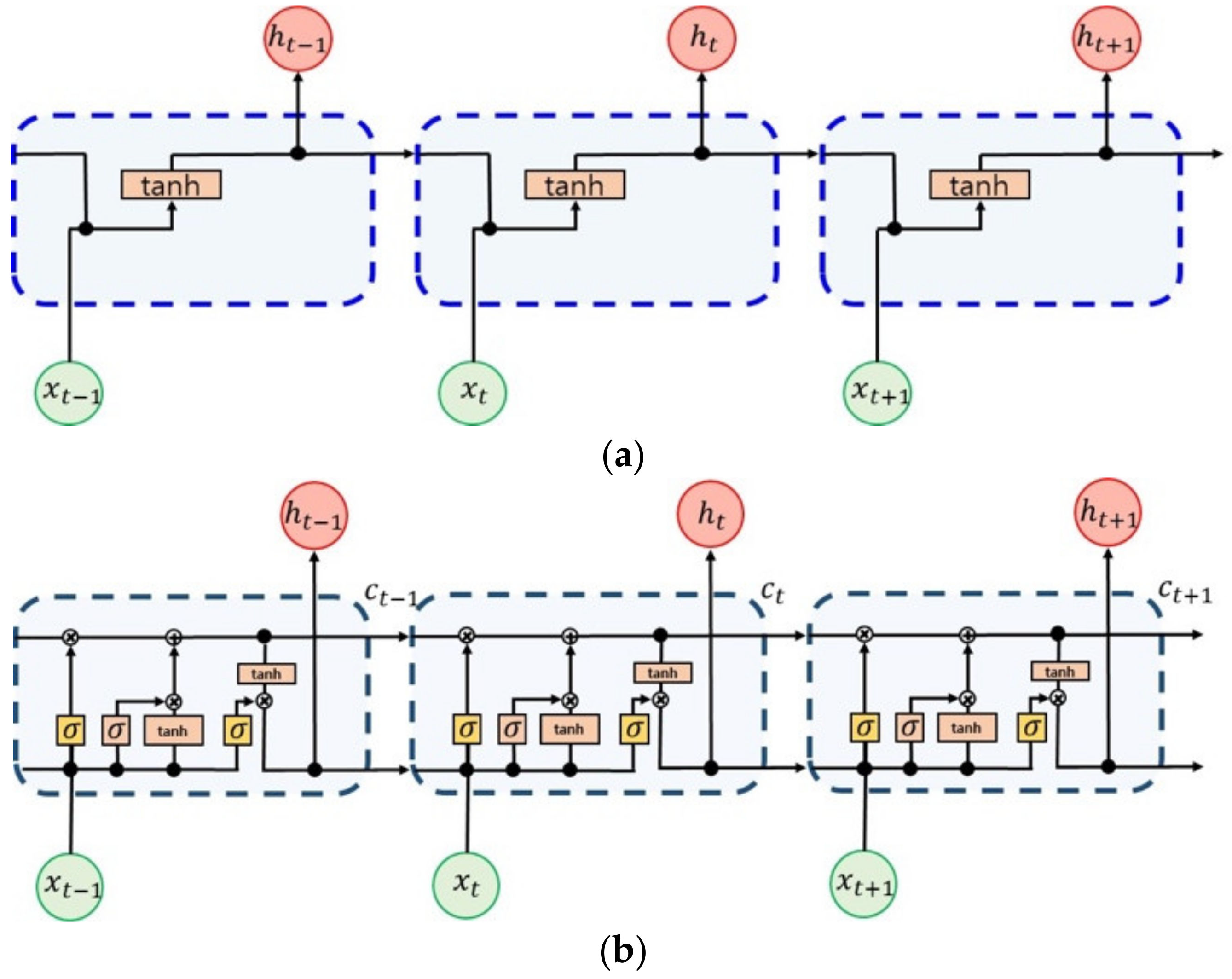
• Recurrent Neural Networks (RNNs)

In the MLP algorithm, values that have passed through the activation function in all hidden layers are directed only toward the output layer. This neural network is called a feedforward neural network. In contrast, recurrent neural networks (RNNs) are characterized by sending the resultant value obtained by the activation function to the input of the next calculation of the hidden layer node. Figure 5 shows a block diagram of the architecture of an RNN. RNNs are mainly used for the analysis of time series data. The difference between an RNN and an MLP is that an RNN has a “recall” (i.e., a hidden state); the current weight value can be regarded as a summary of the input data up to the current point in time. For every new input, each node gradually updates its weight. Finally, after processing all the input data, the weight value remaining in the cell summarizes the entire sequence; when processing data, the output is derived based on the recall of all data up to the present time.

In order to calculate the hidden state at the current time t (denoted as h_t), the weight ${\omega }_x$ for the input value, and the weight ${\omega }_h$ for the hidden state value h_t−1 at time t − 1 are required. The variable h_t can be calculated by [28]

$$h_t=\tan \mathrm{h}\left({\omega }_x{x}_t+{\omega }_h{h}_{t-1}+b\right),$$

(7)

Based on the above, using the hidden layer state and weight ${\omega }_y$, y_t (which is passed to the output layer) is represented as

$$y_t=\max \left(0,{\omega }_y{h}_t+b\right).$$

(8)

Here, the ReLU function was used as a nonlinear activation function in the same way as the MLP algorithm.

• Long Short-Term Memory (LSTM)

In RNNs, as the distance between the input data and the current output data increases, the gradient gradually decreases in the backpropagation, leading to a significant decrease in learning performance. LSTM is an algorithm that resolves this problem. In LSTM, the cell state is added to the hidden state. In RNNs, the information of the previous hidden state is directly used. In LSTM, the gradient is propagated even with increasing information using the forget gate and input gate. For comparison, block diagrams of the LSTM and RNN algorithms are shown in Figure 6.

In the forget gate, the past state information is selected. Using a sigmoid function, a value between 0 and 1 is used to adequately reflect the past state information. That is, if the value is 0, the information of the previous state is forgotten, and if the value is 1, the information of the previous state is fully remembered. The forget gate can be represented as [29]

$$f_t=\mathsf{\sigma }\left({\omega }_{xh\_f}{x}_t+{\omega }_{hh\_f}{h}_{t-1}+b_{h\_f}\right).$$

(9)

The input gate is used to remember the present state information. Using the hidden state value (h_t−1) of the previous step and the present state data, the strength and direction of the current data can be calculated as

$$i_t=\mathsf{\sigma }\left({\omega }_{xh\_i}{x}_t+{\omega }_{hh\_i}{h}_{t-1}+b_{h\_i}\right)$$

(10)

$$o_t=\mathsf{\sigma }\left({\omega }_{xh\_o}{x}_t+{\omega }_{hh\_o}{h}_{t-1}+b_{h\_o}\right)$$

(11)

The LSTM equation reflecting the forget gate and input gate can be represented as

$$g_t=\tan \mathrm{h}\left({\omega }_{xh\_g}{x}_t+{\omega }_{hh\_g}{h}_{t-1}+b_{h\_g}\right),$$

(12)

$$c_t=f_t\odot c_{t-1}+i_t\odot g_t,$$

(13)

$$h_t=o_t\odot \tan \mathrm{h}(c_t),$$

(14)

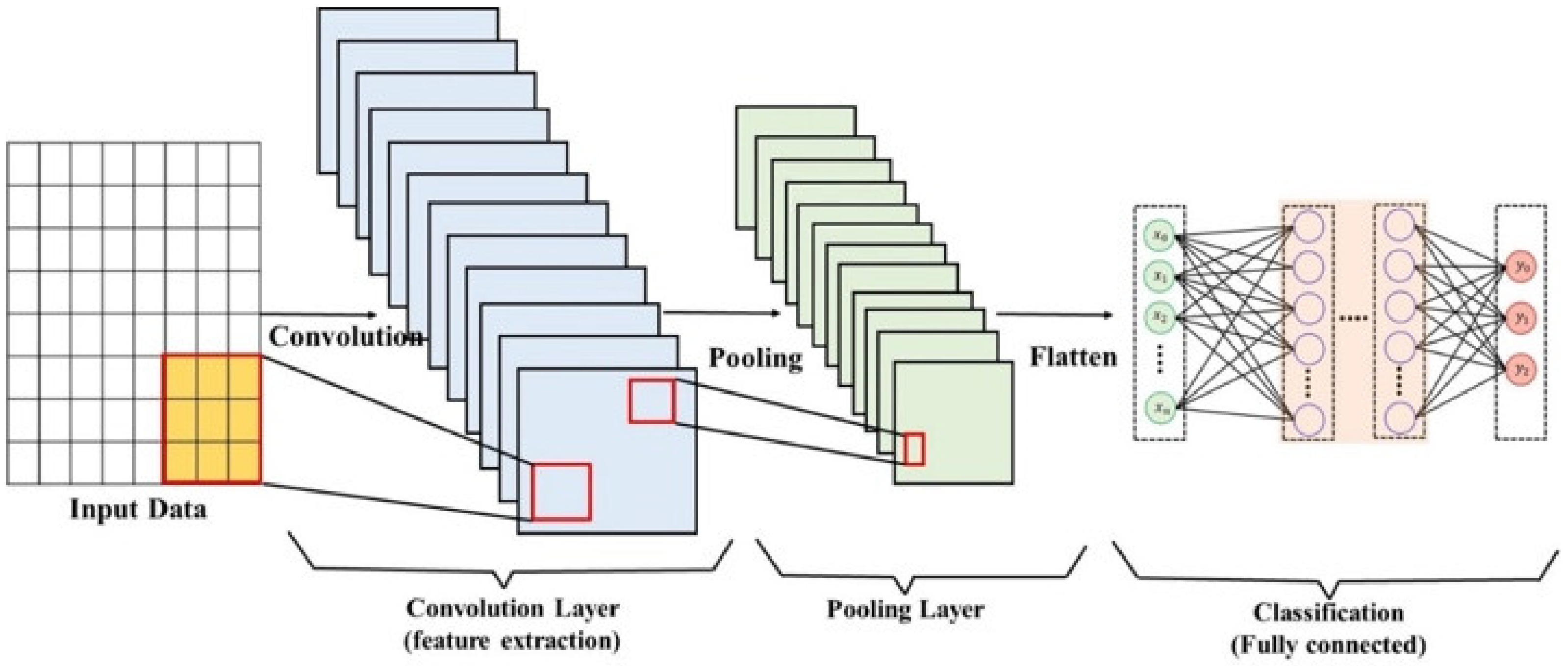
• Convolution Neural Networks (CNN)

The CNN algorithm has similar characteristics to the MLP algorithm and it applies filters to extract local features. Based on the features of the extracted data, a pooling operation is performed with max pooling or average pooling and the result is sent to the next layer. The output is generated using the above process. Figure 7 shows the architecture used in CNNs.

The input data are composed of a matrix and the features of the input data are extracted through the convolution of the input matrix and the filter matrix. From the input data, the surrounding components of each component are examined to identify features and the dimensionality of the data is reduced with the identified features. With the extracted data, the information is pooled through max pooling or average pooling. In this way, the data dimensionality can be reduced and noise can be removed without losing the features [30].

4. Construction of Turbine Rotational Speed Prediction Model

4.1. Data-Based Prediction Technology

Based on the training data, a model for predicting the turbine’s rotational speed was constructed. The data for the OWC-WEC located west of Jeju, South Korea were used as training data. Figure 8 shows photographs of the turbine system and valve system for rated control as well as the power converter and powerline communication (PLC) for load control.

For the composition of the training data, flow velocity data, and pressure data in the turbine input, the mechanical torque and electrical power output were used. Considering the sensor measurement delay and valve operating time, the turbine’s rotational speed after two seconds was predicted for rated control. The turbine rotational speed was changed by the mechanical and electrical torques generated by the input energy based on the equation of motion. Accordingly, parameters that affect the mechanical and electrical torque were selected as training datasets for predicting the turbine’s rotational speed. For the selection of training datasets, data obtained from the operation of real WECs were used. For comparing the performance of each algorithm, several other ocean energy datasets were used for verification. The training datasets used (26 April 2019, 20 July 2019, and 16 August 2019) are shown in Figure 9.

Based on the training datasets, the turbine’s rotational speed 2 s after the present time is predicted. Based on the predicted results, the valve is operated to control the energy input sent to the turbine. The conventional rated control is based on the current rotational speed of the turbine, but if the turbine’s rotational speed can be predicted in advance by reducing the sensor delay and valve operation time, a more precise rated control is possible. Thus, by overcoming the highly volatile nature of wave energy, the operating time and power generation performance can be improved.

4.2. Analysis of Data Correlation

Among the available methods for selecting training datasets, the correlation plot is an intuitive tool for examining the correlation between the input and output data. The NN table was used to comprehensively represent the predictions of the regression model, where N represents the number of training data points. In general, the direction and type of correlations between the data can be identified before conducting a detailed analysis. Figure 10 shows the correlation plots for the training datasets.

The correlation between the output data and the training data can be analyzed based on the colors and numbers in Figure 10. The closer the color is to red and the number is to 1, the higher the correlation between the input and output data. Although all data affect the output value, the turbine’s rotational speed is highly correlated with the turbine’s input flow velocity, mechanical torque, and power generation.

4.3. Model Training with Training Datasets

In deep learning algorithms, a model that predicts the output data based on training data is constructed. There are a number of parameters for model training. The mean squared error is used for model evaluation to update the weights of the model. The loss model used for the model evaluation is

$$\mathrm{MSE}=\frac{1}{N}\sum {\left(Y_A-Y_P\right)}^2,$$

(15)

where $Y_A$ is an actual value, $Y_P$ is a predicted value, and N is the sample size. A low MSE value is an indicator of a well-trained model. The weight update period is optimized using the Adam function in the KERAS optimizer, which is an advanced gradient descent method.

4.4. Seperation of Training Dataset and Test Dataset

The datasets used to verify this model were divided into training and test datasets. The power output data of the OWC-WEC located west of Jeju were used for training. With the 26 April 2019, 20 July 2019, and 16 August 2019 datasets, the performances of each algorithm according to different oceanic conditions were compared. All datasets were originally composed of one hour of data and the training datasets were composed using the first 40 min of data in each dataset. The test datasets were composed using the remaining 20 min in each dataset. The data were sampled at 20 Hz. The datasets used were time series data that included the flow velocity through the turbine, the pressure on the turbine, the mechanical torque, and the power generation output. Figure 11 shows the composition of the training and test datasets.

5. Results and Discussion

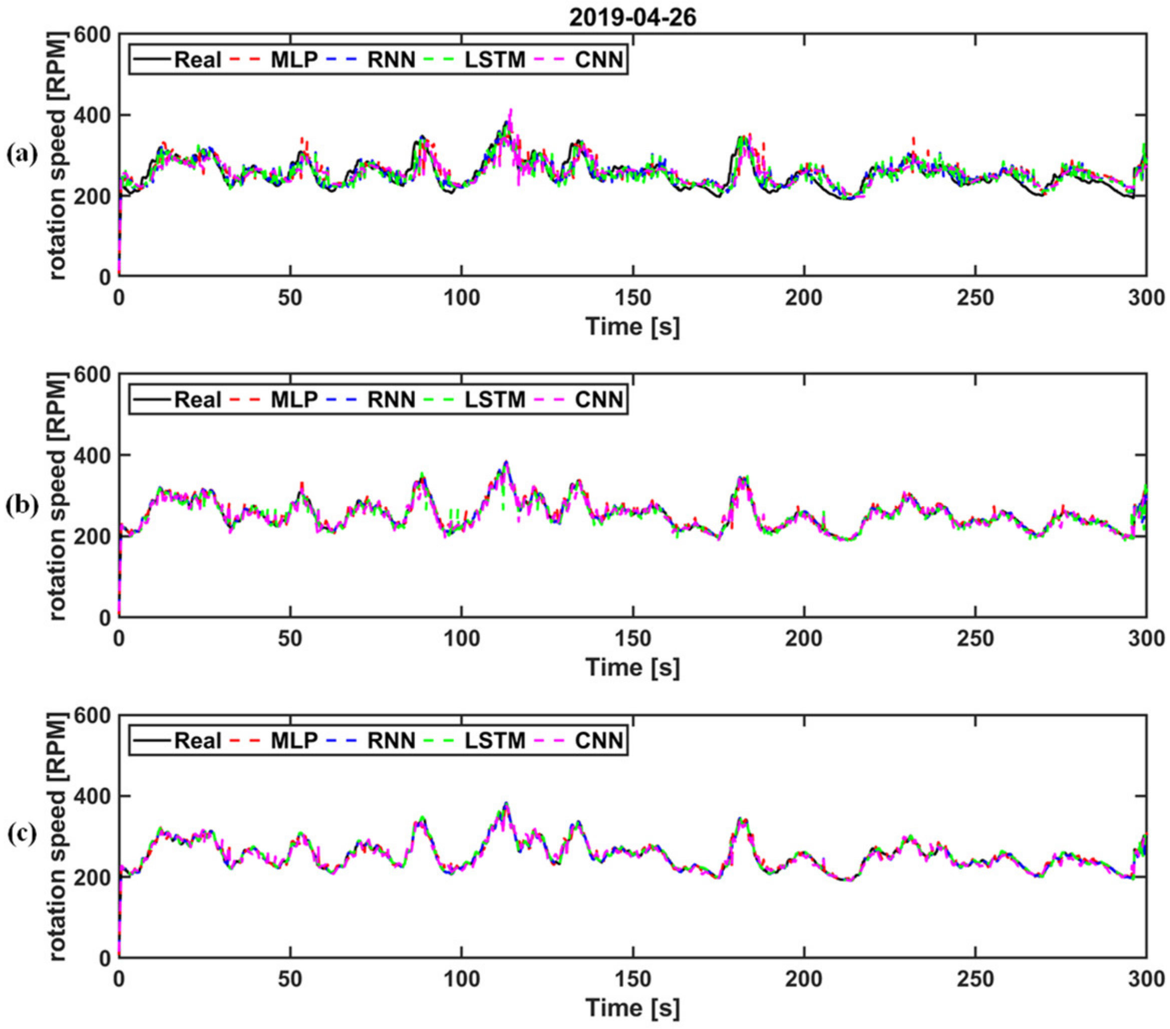
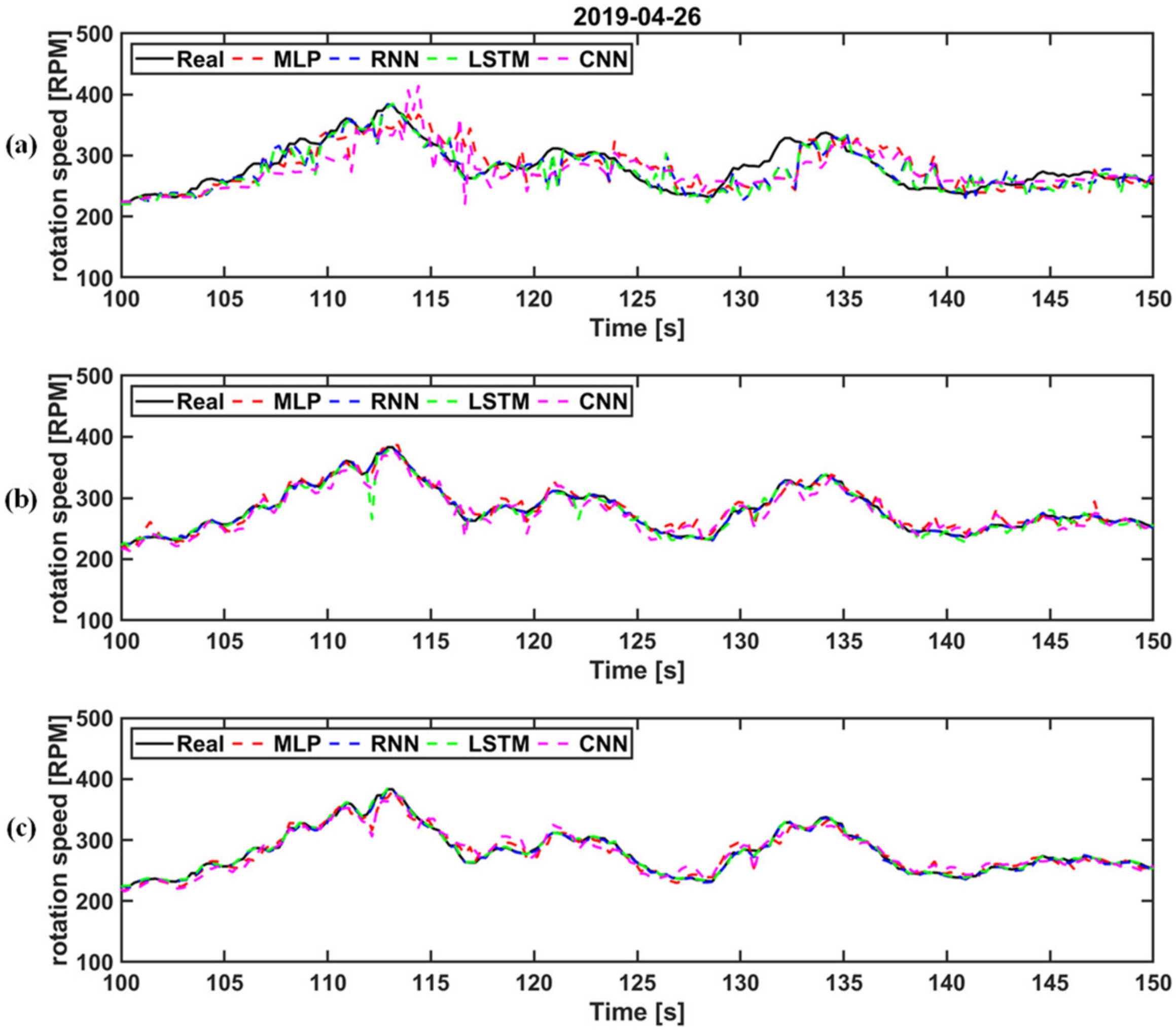
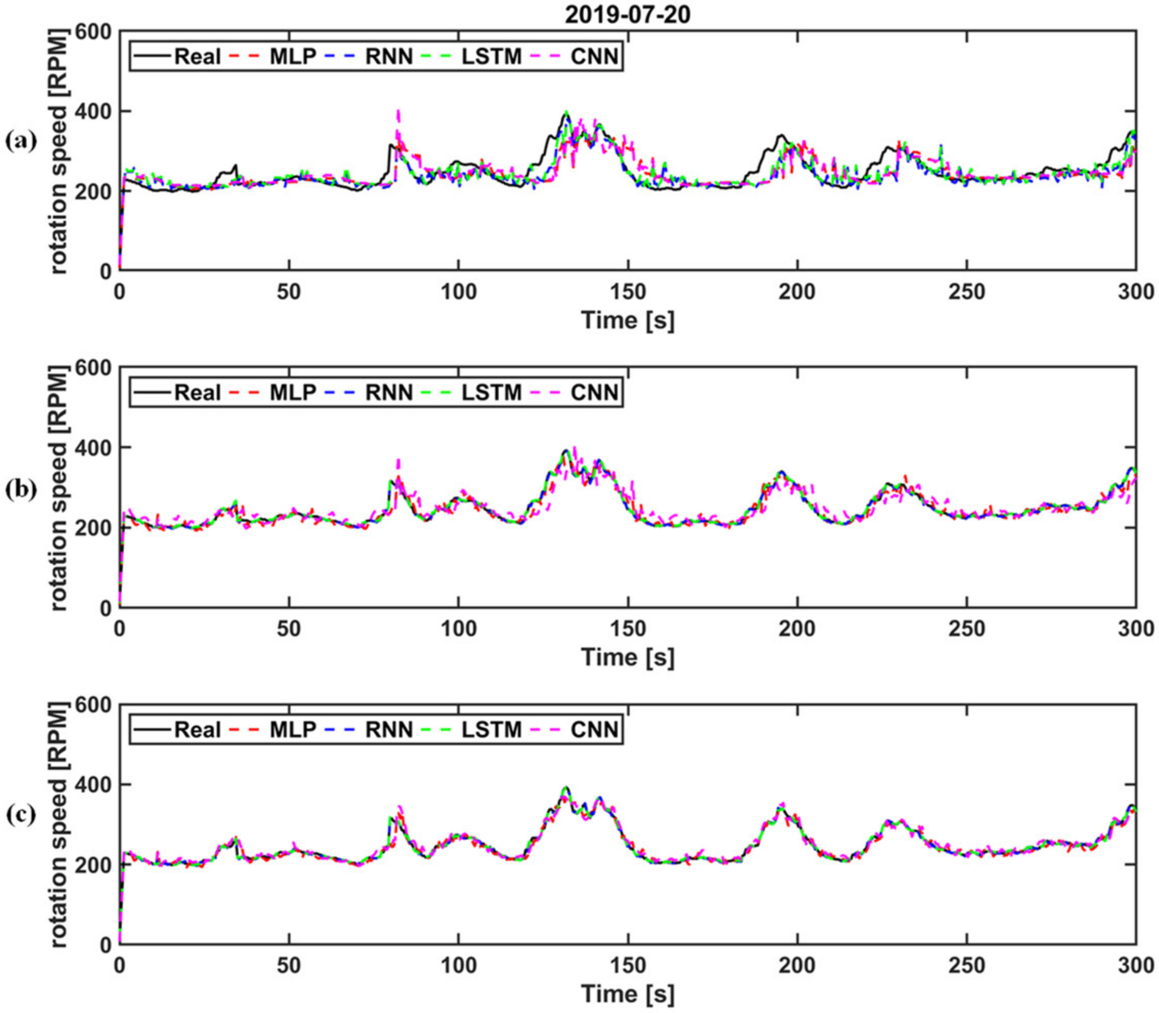
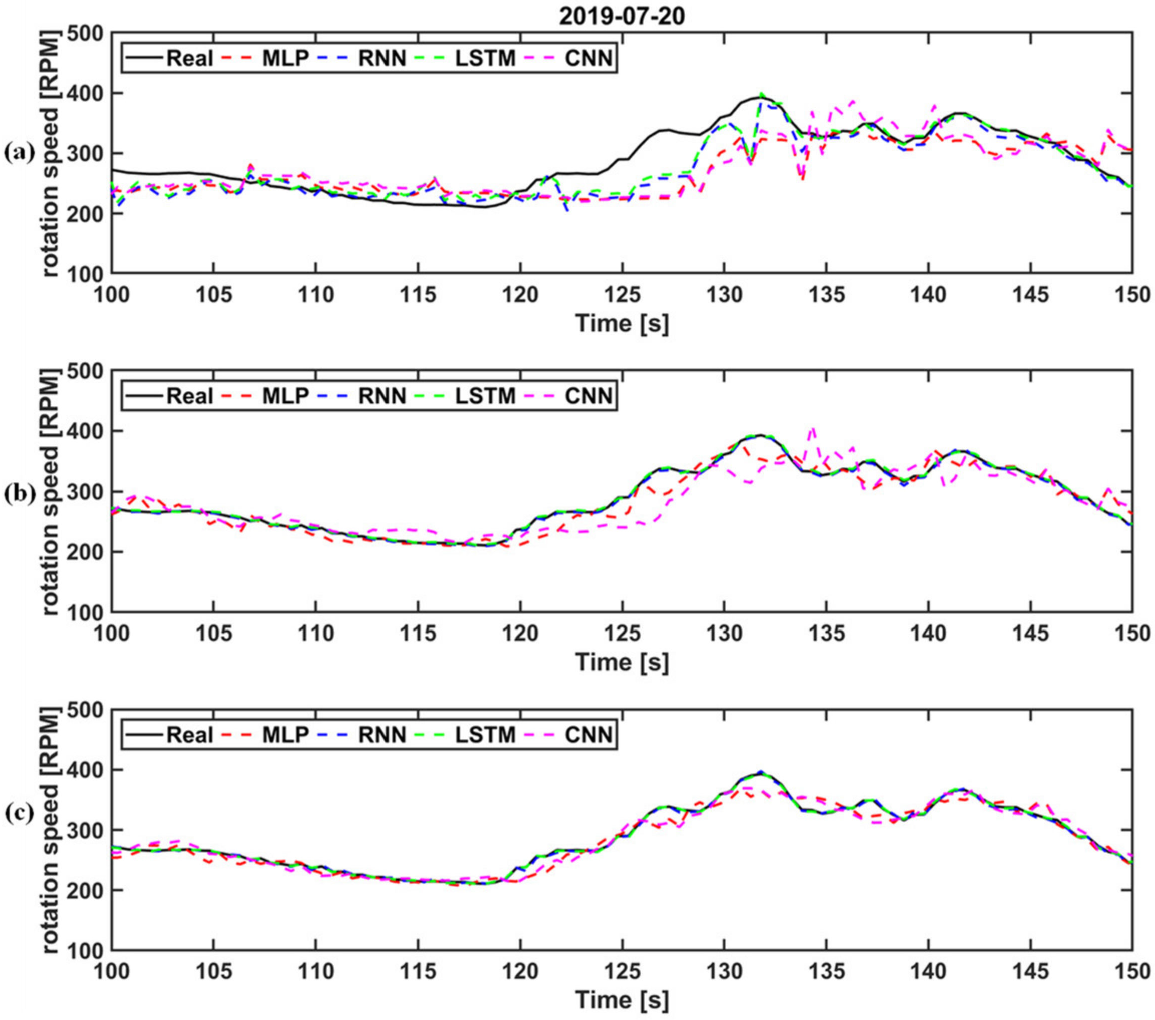
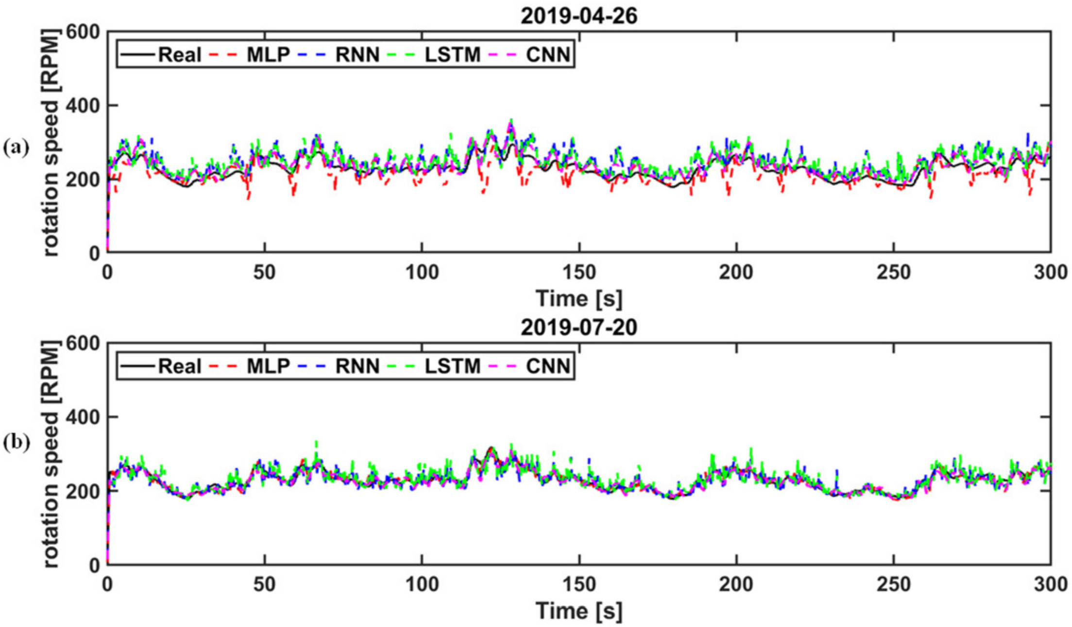
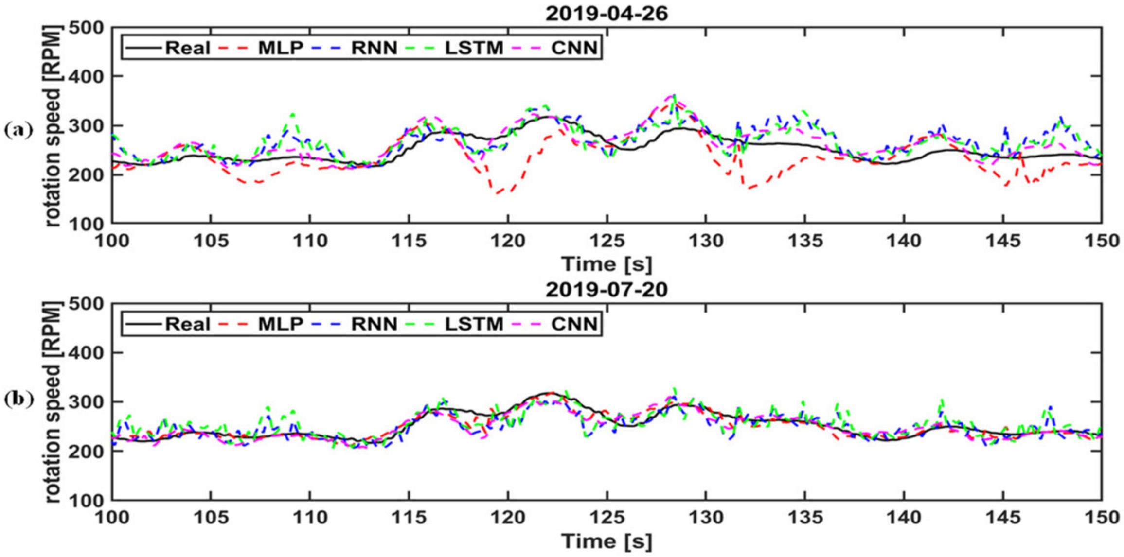
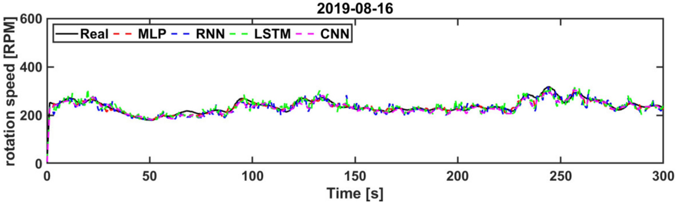
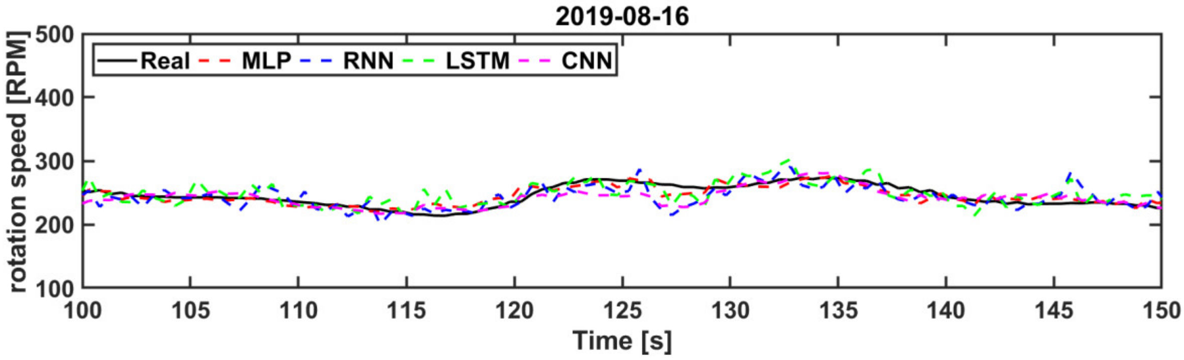
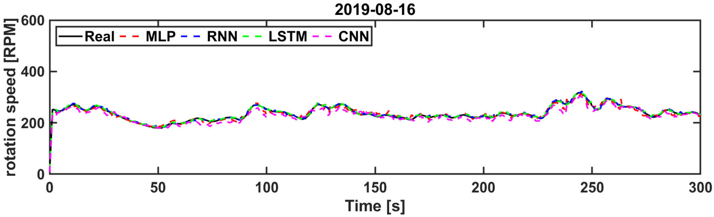
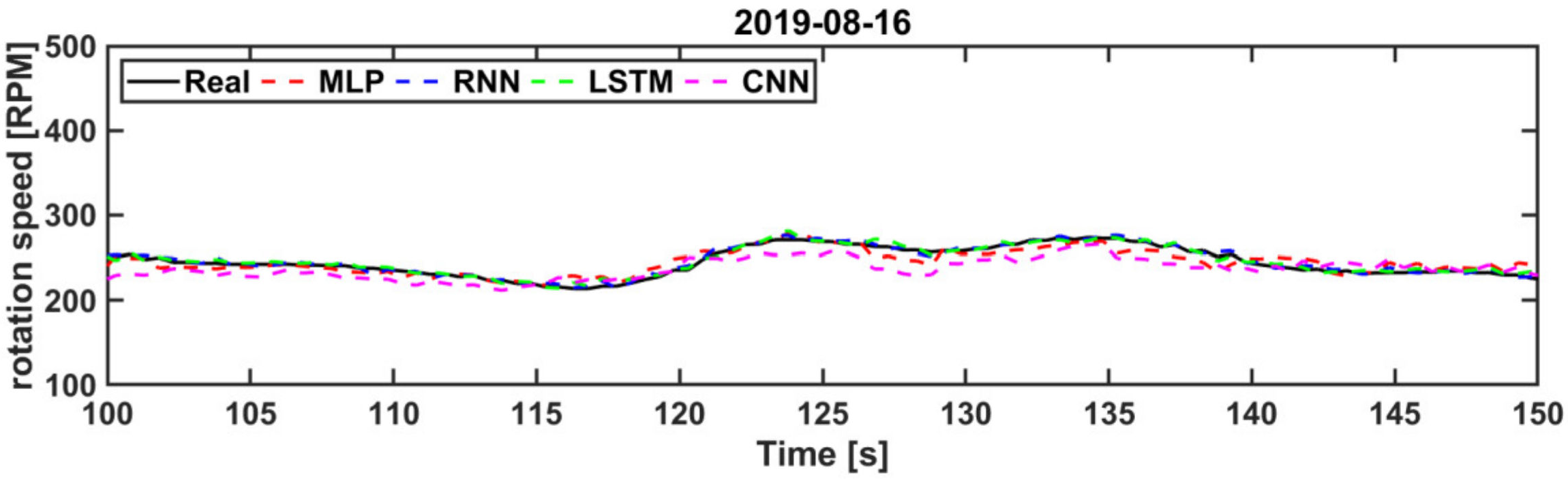
5.1. Comparison of Prediction Results

Table 1. Comparison of prediction results for each case.

	Case	Training Dataset	Test Dataset	Number of Input Datasets
Number of input training datasets	1	Da	Da	2
				6
				10
	2	Db	Db	2
				6
				10
Number of input training datasets	3	Da	Dc	10
	4	Db	Dc	10
	5	Da, Db	Dc	10
	6	Da, Db, Dc	Dc	10

shows the comparison between the prediction results for various cases using different combinations of the training datasets shown in Figure 11. The 26 April 2019, 20 July 2019, and 16 August 2019 datasets are represented as Da, Db, and Dc, respectively.

First, the prediction performance of the deep learning algorithms (MLP, RNN, LSTM, and CNN) for the turbine’s rotational speed as a function of the change in the number of training datasets was analyzed. In addition, the prediction performance was analyzed when the amount of training data was insufficient.

One of the system characteristics is a sensor measurement time delay of about 0.2 s and a valve operating time of about 1.5 s. Thus, when the change in the turbine’s rotational speed after 2 s is predicted in advance using the current input data, the precise control of the valve can be achieved, allowing for the rated control of the power generation output.

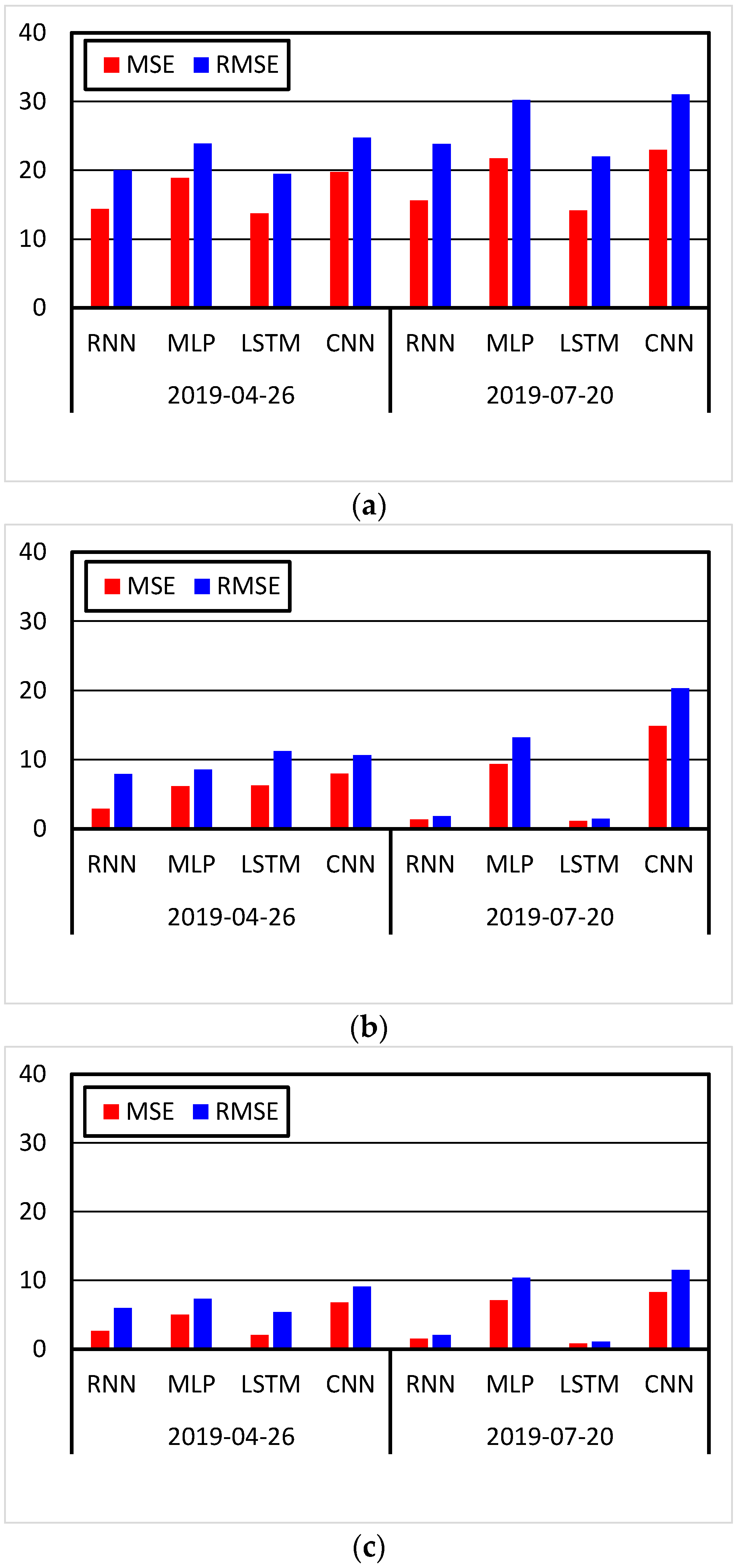
• Deep learning algorithm performance analysis as a function of the number of input training datasets

Figure 12 shows the learning performance as a function of the number of input datasets for the training results applicable to Case 1 in Table 1. The prediction results for each algorithm were compared to the actual data after 2 s. Figure 12a shows the training results when using the two datasets with the highest correlation. For the training data, the mechanical torque and power output were selected. Although there were slight differences in performance between the algorithms, it is clear that the predicted result did not agree with the actual data. The change in the turbine’s rotational speed was more influenced by data other than the mechanical torque and power output. This can be confirmed through the amplified waveforms shown in Figure 13a.

Figure 12b shows the performance of each algorithm when using six highly correlated datasets. For the training data, the input flow velocity through the turbine, mechanical torque, and power output were selected. As the RNN and LSTM algorithms make predictions based on the recall of past data, it was first necessary to confirm that the results from both algorithms accurately matched the actual data. In particular, the LSTM algorithm exhibited superior performance because the learning performance was not reduced during backpropagation. However, the CNN algorithm did not accurately exhibit the characteristics expected with a decrease in the number of input datasets, indicating that the learning performance was reduced. This can be confirmed through the amplified waveforms shown in Figure 13b.

Figure 12c shows the performance results when using all training datasets. In this case, all the deep learning algorithms made accurate predictions. Although the differences were not significant, the RNN and LSTM algorithms, which remember information from past states, demonstrated superior performance. The CNN algorithm recognizes the correlation between the features of the datasets and predicts the output data based on the correlation. However, the correlation between the datasets used in this study was low, which caused the CNN algorithm to exhibit the lowest learning performance. This can be confirmed through the amplified waveforms shown in Figure 13c.

Figure 14 shows the learning performance as a function of the number of input datasets for the training results applicable to Case 2 in Table 1. The prediction results of each algorithm were compared to the actual data after 2 s. Similar to the case in Figure 12, Figure 14a shows the training results when using the two datasets with the highest correlation. For the training data, the mechanical torque and power output were selected, as in Figure 12a. Although there were slight differences in performance between the algorithms, the predicted result did not agree with the actual data. This can be confirmed through the amplified waveforms shown in Figure 15b. This finding is identical to the results shown in Figure 12a.

Figure 14b shows the results of the training using six datasets with a high correlation. For the training data, the input flow velocity through the turbine, mechanical torque, and power output were selected. The LSTM algorithm exhibited the highest accuracy. For the CNN algorithm, the data features were not accurately extracted, leading to a poor match with the actual data. This can be confirmed through the amplified waveforms shown in Figure 15b.

Figure 14c shows the results obtained from using the entire training dataset. Accurate predictions were achieved by all the deep learning algorithms. The RNN and LSTM algorithms exhibited superior performance. For the CNN algorithm, the feature identification between the datasets was difficult due to using training data with low correlation, causing it to exhibit the lowest learning performance. This can be confirmed through the amplified waveforms shown in Figure 15c.

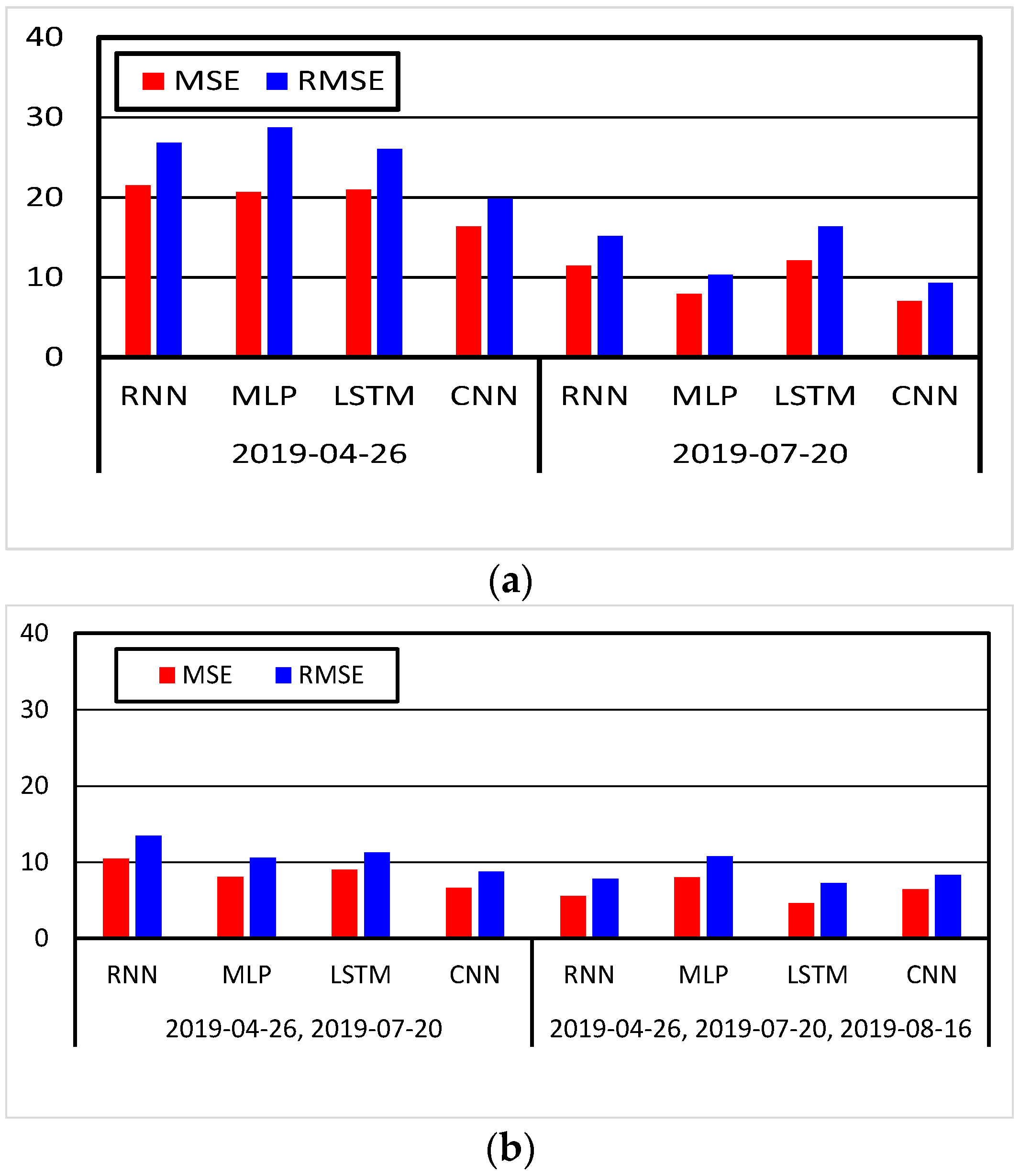
• Deep learning algorithm performance analysis as a function of the number of training datasets

Figure 16 shows the training results applicable to Cases 3 and 4, as listed in Table 1. The training was performed with the 26 April 2019 and 20 July 2019 datasets to predict the 16 August 2019 dataset. That is, the oceanic conditions of one date were predicted based on the training with datasets for different oceanic conditions, and the prediction performance was compared for each algorithm. For Figure 16a, the training was performed with the 26 April 2019 dataset and predictions were made for data from 16 August 2019. For Figure 16b, the training was performed with the 20 July 2019 dataset and predictions were made for data from 16 August 2019. The trends for the two cases are similar, but the results indicate that a sufficiently large amount of data is required for training in order to predict the turbine’s rotational speed in different oceanic conditions. As shown in Figure 17, most algorithms did not make accurate predictions. However, the training result for the 20 July 2019 dataset achieved a better prediction performance than the training result for the 26 April 2019 dataset. This indicates that the higher the similarity between the training dataset and the dataset used for prediction, the more accurate the prediction performance. In addition, in the case of an insufficient amount of training data being available for the prediction of different oceanic conditions, the CNN algorithm exhibited a better performance than the LSTM algorithm, which showed superior performance in the previous case.

Figure 18 shows the training results applicable to Case 5, which is shown in Table 1. The training was performed with the 26 April 2019 and 20 July 2019 datasets to predict the 16 August 2019 dataset. As shown in Figure 16 and Figure 17, when the training was performed with two days of data, the predicted values after 2 s were more accurate (unlike the result obtained from training with one day of data). As can be seen in Figure 19, the higher the similarity between the training dataset and the dataset to be predicted, the more accurate the prediction performance. When there is little similarity between the two datasets, the prediction performance decreases. In particular, the performance of the LSTM algorithm is significantly lowered.

Figure 20 shows the training results applicable to Case 6, which is also shown in Table 1. The training was performed with all datasets (three days) to predict the 16 August 2019 dataset. The 16 August 2019 dataset that was trained and the 16 August 2019 dataset that was predicted were categorized as training data and test data. Compared to all other results, when the training was performed with all datasets, a more accurate prediction performance was achieved after 2 s. As all datasets used for training were similar to the predicted results, an accurate prediction performance was achieved, as shown in Figure 21. In addition, the LSTM model showed the most accurate prediction performance when datasets with high similarity were used. A more detailed performance comparison for each case is performed in the next subsection using the error analysis method.

5.2. Discussion on Various Deep Learning Model Results

The error analysis method, which is a commonly used evaluation method for deep learning models, was used for a more detailed analysis of the performance of the deep learning algorithms. The mean absolute error (MAE) and root mean square error (RMSE) were used for the error analysis. The performances of the MLP, RNN, LSTM, and CNN algorithms were compared using the error analysis method.

First, the mean absolute error (MAE) was calculated using the mean value of the absolute difference between the actual and predicted values. The equation for calculating the MAE is

$$\mathrm{MAE}=\frac{1}{N}\sum \left|Y_A-Y_P\right|,$$

(16)

where $Y_A\mathrm{and}{Y}_P$ represent the actual data and the predicted result, respectively, and N represents the number of datasets used for the evaluation.

The RMSE was calculated using the root of the mean of the squared differences between the actual and predicted values. This error analysis method is commonly used to analyze the difference between the predicted value of the model and the value measured in an actual environment. The RMSE is calculated as

$$\mathrm{RMSE}=\sqrt{\frac{1}{N}\sum {\left(Y_A-Y_P\right)}^2}.$$

(17)

The prediction performances of the algorithms were compared in terms of the MAE and RMSE. Through the analysis, a deep learning algorithm and dataset composition that are suitable for predicting the turbine’s rotational speed for valve control were determined.

5.3. Model Performance Comparison

The performance evaluation of the deep learning algorithms (MLP, RNN, LSTM, and CNN) was conducted by applying the error analysis method described above. In addition, the performances of the algorithms were compared by applying the error analysis method to each case, as shown in Table 1.

Figure 22 shows the plot of the prediction performance for each algorithm as a function of the number of input datasets for the conditions of Cases 1 and 2, which are shown in Table 1. For the performance of each algorithm, the MAE and RMSE were used to compare the errors between the actual and predicted values.

Although there were differences in the error values of the algorithms between the cases, the prediction performance of the algorithms increases as the number of training datasets increases. In particular, the LSTM algorithm showed the most accurate prediction results. This indicates that regardless of the date of the training dataset, the error of the LSTM algorithm was the lowest for both the MAE and RMSE. However, the error of the CNN algorithm was the largest. This is because the CNN algorithm did not accurately extract features due to the lack of the number of input data. The LSTM algorithm was the best performer, RNN was the second best, MLP was third, and CNN performed the worst. In addition, as the number of training datasets decreased, the learning performance was reduced, which confirms that the prediction performance is improved by considering more data.

Figure 23 shows the learning performance of each algorithm as a function of the amount of data for the conditions of Cases 3 and 4. Figure 23a shows the result of training using the training dataset of one day (either 26 April 2019 or 20 July 2019) for predicting the 16 August 2019 dataset. As shown in Figure 23a, when the similarity between the training dataset and the prediction dataset was low, the CNN algorithm showed the best performance. In addition, the results confirm that as the similarity between the data for the date to be predicted and training data increases, the error value decreases (i.e., training using the 20 July 2019 dataset showed lower error values than those using the 26 April 2019 dataset).

Figure 23b shows the prediction performance of each algorithm as a function of the amount of data for the conditions of Cases 5 and 6. The figure shows the result of predicting the 16 August 2019 dataset with more training data than was used for Figure 23a. When the amount of data was increased compared to that in Figure 23a, the prediction performance improved. In addition, using three days of data generated a superior performance compared to using two days of data. However, in the case of the MLP algorithm, the performance was slightly reduced. This is likely to require an analysis based on more data.

In addition, in the case of using two days of data, when the similarity between the training data and the prediction data was low, the CNN algorithm demonstrated superior performance compared to the LSTM algorithm (similar to the case of using one day of data). However, when using three days of data (instead of using two days of data), the LSTM algorithm showed the best performance because the similarity between the training data and the prediction data increased. The analysis of the various input data conditions indicates that the performance of the algorithms changed according to the similarity between the training data and the prediction data. With more similarity, the LSTM algorithm showed the best performance, and with less similarity, the CNN algorithm showed the best performance. The performance rankings for each algorithm according to each case are listed in

Table 2. Performance ranking for each algorithm according to changes in training data.

	Case	Training Data	Test Data	Number of Input Data	MLP	RNN	LSTM	CNN
Number of input training data	1	Da	Da	2	3	2	1	4
				6	3	1	2	4
				10	3	2	1	4
	2	Db	Db	2	3	2	1	4
				6	3	2	1	4
				10	3	2	1	4
Amount of input training data	3	Da	Dc	10	4	3	2	1
	4	Db	Dc	10	2	3	4	1
	5	Da, Db	Dc	10	1	4	3	2
	6	Da, Db, Dc	Dc	10	3	2	1	4

.

In conclusion, even with changing oceanic conditions, the turbine’s rotational speed can be predicted for valve control using deep learning algorithms. In addition, with an increased number of training datasets with various features, the prediction performance for new input data can be improved. The higher the similarity between the training data and the prediction data, the better the LSTM algorithm performed. If more data become available in the future, it will be possible to perform more tests and verify the superior performance of the LSTM algorithm.

6. Conclusions

In this study, we presented the results of predicting the instantaneous rotational speed of a turbine generator based on a deep learning algorithm for the rated power control of an OWC-WEC. We compared the prediction performance for the instantaneous rotational speed of a turbine generator by applying various AI-based deep learning algorithms using the operation data of an OWC-WEC located west of Jeju, South Korea. As the conventional rated control method is based on the instantaneous rotational speed of the turbine generator in its present state, the control can only be performed after the energy input surpasses the rated value of the system. Therefore, in this study, a deep learning algorithm was applied to predict the instantaneous rotational speed of a turbine generator in advance. Based on this prediction, a rated control algorithm was proposed that operates the valve before the energy input reaches higher than the rated value. To achieve an accurate prediction performance for a more refined rated power control, various deep learning algorithms were applied and the performances of the algorithms were compared in detail using an error analysis method. In addition, we compared the prediction performance of each algorithm according to the type of training data. The results showed that regardless of the input conditions and type of training data, the LSTM algorithm exhibited the most accurate prediction for the actual instantaneous rotational speed of the turbine generator, and the result was not significantly affected by the change in the type of training data. However, when the data correlation was low, it was confirmed that the results of the CNN algorithm were excellent. In conclusion, as a result of this study, it was possible to predict the instantaneous rotation speed of the turbine generator after 2 s for rating control by applying a deep learning algorithm.

References

1. Yan, J. Transitions of the future energy systems: Editorial of year 2013 for the 101, volume of applied energy. Appl. Energy 2013, 101, 1–2. [Google Scholar] [CrossRef]
2. Krajačić, G.; Duić, N.; da Graça Carvalho, M. How to achieve a 100% RES electricity supply for Portugal? Appl. Energy 2011, 88, 508–517. [Google Scholar] [CrossRef]
3. Papaefthymiou, G.; Dragoon, K. Towards 100% renewable energy systems: Uncapping power system flexibility. Energy Policy 2016, 92, 69–82. [Google Scholar] [CrossRef]
4. Alizadeh, M.; Moghaddam, M.P.; Amjady, N.; Siano, P.; Sheikh-El-Eslami, M. Flexibility in future power systems with high renewable penetration: A review. Renew. Sustain. Energy Rev. 2016, 57, 1186–1193. [Google Scholar] [CrossRef]
5. Wang, J.; Conejo, A.J.; Wang, C.; Yan, J. Smart grids, renewable energy integration, and climate change mitigation—Future electric energy systems. Appl. Energy 2012, 96, 1–3. [Google Scholar] [CrossRef]
6. Mork, G.; Barstow, S.; Kabuth, A.; Pontes, M.T. Assessing the global wave energy potential. In Proceedings of the International Conference on Offshore Mechanics and Arctic Engineering, Shanghai, China, 20 December 2010; pp. 447–454. [Google Scholar]
7. Esteban, M.; Leary, D. Current developments and future prospects of offshore wind and ocean energy. Appl. Energy 2012, 90, 128–136. [Google Scholar] [CrossRef]
8. Glendenning, I. Ocean wave power. Appl. Energy 1977, 3, 197–222. [Google Scholar] [CrossRef]
9. Falcão, A.F.; Henriques, J.C. Oscillating-water-column wave energy converters and air turbines: A review. Renew. Energy 2016, 85, 1391–1424. [Google Scholar] [CrossRef]
10. Falcão, A.D.O. The shoreline OWC wave power plant at the Azores. In Proceedings of the 4th European Wave Energy Conference, Aalborg, Denmark, 4–6 December 2000. [Google Scholar]
11. Heath, T.V. The development and installation of the Limpet wave energy converter. In World Renewable Energy Congress VI; Pergamon Press: Oxford, UK, 2000; Chapter 334; pp. 1619–1622. [Google Scholar] [CrossRef]
12. Torre-Enciso, Y.; Ortubia, I.; De Aguileta, L.L.; Marqués, J. Mutriku wave power plant: From the thinking out to the reality. In Proceedings of the 8th European Wave Tidal Energy Conference, Uppsala, Sweden, 7–10 September 2009; pp. 319–329. [Google Scholar]
13. Mala, K.; Badrinath, S.N.; Chidanand, S.; Kailash, G.; Jayashankar, V. Analysis of power modules in the Indian wave energy plant. In Proceedings of the Annual IEEE India Conference, Ahmedabad, India, 18–20 December 2009; pp. 1–4. [Google Scholar] [CrossRef]
14. Alcorn, R.; Blavette, A.; Healy, M.; Lewis, A.; Raymond, A.; Anne, B.; Mark, H.; Anthony, L. FP7 EU funded CORES wave energy project: A coordinators’ perspective on the Galway Bay sea trials. Underw. Technol. 2014, 32, 51–59. [Google Scholar] [CrossRef] [Green Version]
15. Yu, Z.; Jiang, N.; You, Y. Load control method and its realization on an OWC wave power converter. In OMAE; ASME: New York, NY, USA, 1994; Volume 1. [Google Scholar]
16. Justino, P.A.P.; de O. Falcaõ, A.F. Rotational Speed Control of an OWC Wave Power Plant. J. Offshore Mech. Arct. Eng. 1999, 121, 65–70. [Google Scholar] [CrossRef]
17. Falcão, A.; Henriques, J.; Gato, L. Rotational speed control and electrical rated power of an oscillating-water-column wave energy converter. Energy 2017, 120, 253–261. [Google Scholar] [CrossRef]
18. Henriques, J.; Gomes, R.; Gato, L.; Falcão, A.; Robles, E.; Ceballos, S. Testing and control of a power take-off system for an oscillating-water-column wave energy converter. Renew. Energy 2015, 85, 714–724. [Google Scholar] [CrossRef]
19. Carrelhas, A.; Gato, L.; Henriques, J.; Falcão, A.; Varandas, J. Test results of a 30 kW self-rectifying biradial air turbine-generator prototype. Renew. Sustain. Energy Rev. 2019, 109, 187–198. [Google Scholar] [CrossRef]
20. Fadare, D. The application of artificial neural networks to mapping of wind speed profile for energy application in Nigeria. Appl. Energy 2010, 87, 934–942. [Google Scholar] [CrossRef]
21. Asrari, A.; Wu, T.X.; Ramos, B. A Hybrid Algorithm for Short-Term Solar Power Prediction—Sunshine State Case Study. IEEE Trans. Sustain. Energy 2016, 8, 582–591. [Google Scholar] [CrossRef]
22. De Paiva, G.M.; Pimentel, S.P.; Alvarenga, B.P.; Marra, E.; Mussetta, M.; Leva, S. Multiple Site Intraday Solar Irradiance Forecasting by Machine Learning Algorithms: MGGP and MLP Neural Networks. Energies 2020, 13, 3005. [Google Scholar] [CrossRef]
23. Hu, J.; Wang, J.; Zeng, G. A hybrid forecasting approach applied to wind speed time series. Renew. Energy 2013, 60, 185–194. [Google Scholar] [CrossRef]
24. Costa, A.; Crespo, A.; Navarro, J.; Lizcano, G.; Madsen, H.; Feitosa, E. A review on the young history of the wind power short-term prediction. Renew. Sustain. Energy Rev. 2008, 12, 1725–1744. [Google Scholar] [CrossRef] [Green Version]
25. More, A.; Deo, M. Forecasting wind with neural networks. Mar. Struct. 2003, 16, 35–49. [Google Scholar] [CrossRef]
26. Ju, C.; Wang, P.; Goel, L.; Xu, Y. A two-layer energy management system for microgrids with hybrid energy storage considering degradation costs. IEEE Trans. Smart Grid 2017, 9, 6047–6057. [Google Scholar] [CrossRef]
27. Hernández-Lobato, J.M.; Adams, R. Probabilistic backpropagation for scalable learning of bayesian neural networks. In Proceedings of the International Conference on Machine Learning, Lille, France, 7–9 July 2015; pp. 1861–1869. [Google Scholar]
28. Yin, X.; Jiang, Z.; Pan, L. Recurrent neural network based adaptive integral sliding mode power maximization control for wind power systems. Renew. Energy 2019, 145, 1149–1157. [Google Scholar] [CrossRef]
29. Cheng, J.; Dong, L.; Lapata, M. Long short-term memory-networks for machine reading. arXiv 2016, arXiv:1601.06733. [Google Scholar]
30. Ghorbanzadeh, O.; Blaschke, T.; Gholamnia, K.; Meena, S.R.; Tiede, D.; Aryal, J. Evaluation of Different Machine Learning Methods and Deep-Learning Convolutional Neural Networks for Landslide Detection. Remote Sens. 2019, 11, 196. [Google Scholar] [CrossRef] [Green Version]
31. Chan, R.; Kim, K.W.; Park, J.Y.; Park, S.W.; Kim, K.H.; Kwak, S.S. Power Performance Analysis According to the Configuration and Load Control Algorithm of Power Take-Off System for Oscillating Water Column Type Wave Energy Converters. Energies 2020, 13, 6415. [Google Scholar] [CrossRef]
32. Khan, P.W.; Byun, Y.-C.; Lee, S.-J.; Park, N. Machine Learning Based Hybrid System for Imputation and Efficient Energy Demand Forecasting. Energies 2020, 13, 2681. [Google Scholar]
Figure 1. Conventional control method for OWC-WECs.
Energies 15 00572 g001
Figure 2. (a) Valve operation mechanism and (b) operating time delay for conventional rated power control.
Energies 15 00572 g002
Figure 3. (a) Conventional valve control method and (b) proposed valve control method for rated power control.
Energies 15 00572 g003
Figure 4. Schematic of a multi-layer perceptron.
Energies 15 00572 g004
Figure 5. Schematic for recurrent neural networks (RNNs).
Energies 15 00572 g005
Figure 6. Comparison of (a) RNN algorithm and (b) LSTM algorithm.
Energies 15 00572 g006
Figure 7. Architecture of convolutional neural networks (CNNs).
Energies 15 00572 g007
Figure 8. (a) Photograph of the OWC-WEC west of Jeju, South Korea. (b) Photographs of the turbine system and valve system. (c) Power converter/PLC and control program. (d) Measurement sensor data information.
Energies 15 00572 g008aEnergies 15 00572 g008b
Figure 9. Training datasets for the application of deep learning algorithms: (a) 26 April 2019, (b) 20 July 2019, and (c) 16 August 2019.
Energies 15 00572 g009
Figure 10. Correlation plots for the training datasets.
Energies 15 00572 g010
Figure 11. Summary of training datasets and test datasets.
Energies 15 00572 g011
Figure 12. Comparison of prediction performance as a function of the number of input datasets for each algorithm (26 April 2019): (a) the two datasets with the highest correlation; (b) six datasets with high correlation; and (c) all training data.
Energies 15 00572 g012
Figure 13. Comparison of amplified prediction performance as a function of the number of input datasets for each algorithm (26 April 2019): (a) the two datasets with the highest correlation; (b) six datasets with high correlation; and (c) all training data.
Energies 15 00572 g013
Figure 14. Comparison of prediction performances as a function of the number of input datasets for each algorithm (20 July 2019): (a) the two datasets with the highest correlation; (b) six datasets with high correlation; and (c) all training data.
Energies 15 00572 g014
Figure 15. Comparison of amplified prediction performances as a function of the number of input datasets for each algorithm (20 July 2019): (a) the two datasets with the highest correlation; (b) six datasets with high correlation; and (c) all training data.
Energies 15 00572 g015
Figure 16. Comparison of the prediction performances of each algorithm for the conditions of Cases 3 and 4. Prediction result of test dataset 16 August 2019 using (a) the 26 April 2019 training dataset and (b) the 20 July 2019 training dataset.
Energies 15 00572 g016
Figure 17. Detailed comparison of the prediction performances of each algorithm for the conditions of Cases 3 and 4. Prediction result of test dataset 16 August 2019 using (a) the 26 April 2019 training dataset and (b) the 20 July 2019 training dataset.
Energies 15 00572 g017
Figure 18. Comparison of the prediction performances of each algorithm for the conditions of Case 5 (training datasets: 26 April 2019, 20 July 2019; test dataset: 16 August 2019).
Energies 15 00572 g018
Figure 19. Detailed comparison of the prediction performances of each algorithm for the conditions of Case 5 (training datasets: 26 April 2019, 20 July 2019; test dataset: 16 August 2019).
Energies 15 00572 g019
Figure 20. Comparison of the prediction performances of each algorithm for the conditions of Case 6 (training datasets: 26 April 2019, 20 July 2019, 16 August 2019; test dataset: 16 August 2019).
Energies 15 00572 g020
Figure 21. Detailed comparison of the prediction performances of each algorithm for the conditions of Case 6 (training datasets: 26 April 2019, 20 July 2019, 16 August 2019; test dataset: 16 August 2019).
Energies 15 00572 g021
Figure 22. Training result error for each algorithm as a function of the number of input datasets for the conditions of Cases 1 and 2: (a) the two datasets with the highest correlation; (b) six datasets with high correlation; and (c) all training data.
Energies 15 00572 g022
Figure 23. Training result errors for each algorithm as a function of the amount of data used for training: (a) prediction results after training with one day of data; (b) prediction results after training with two and three days of data.
Energies 15 00572 g023