
Reliability Updating of Offshore Structures Subjected to Marine Growth


Abstract
1. Introduction
2. Materials and Methods
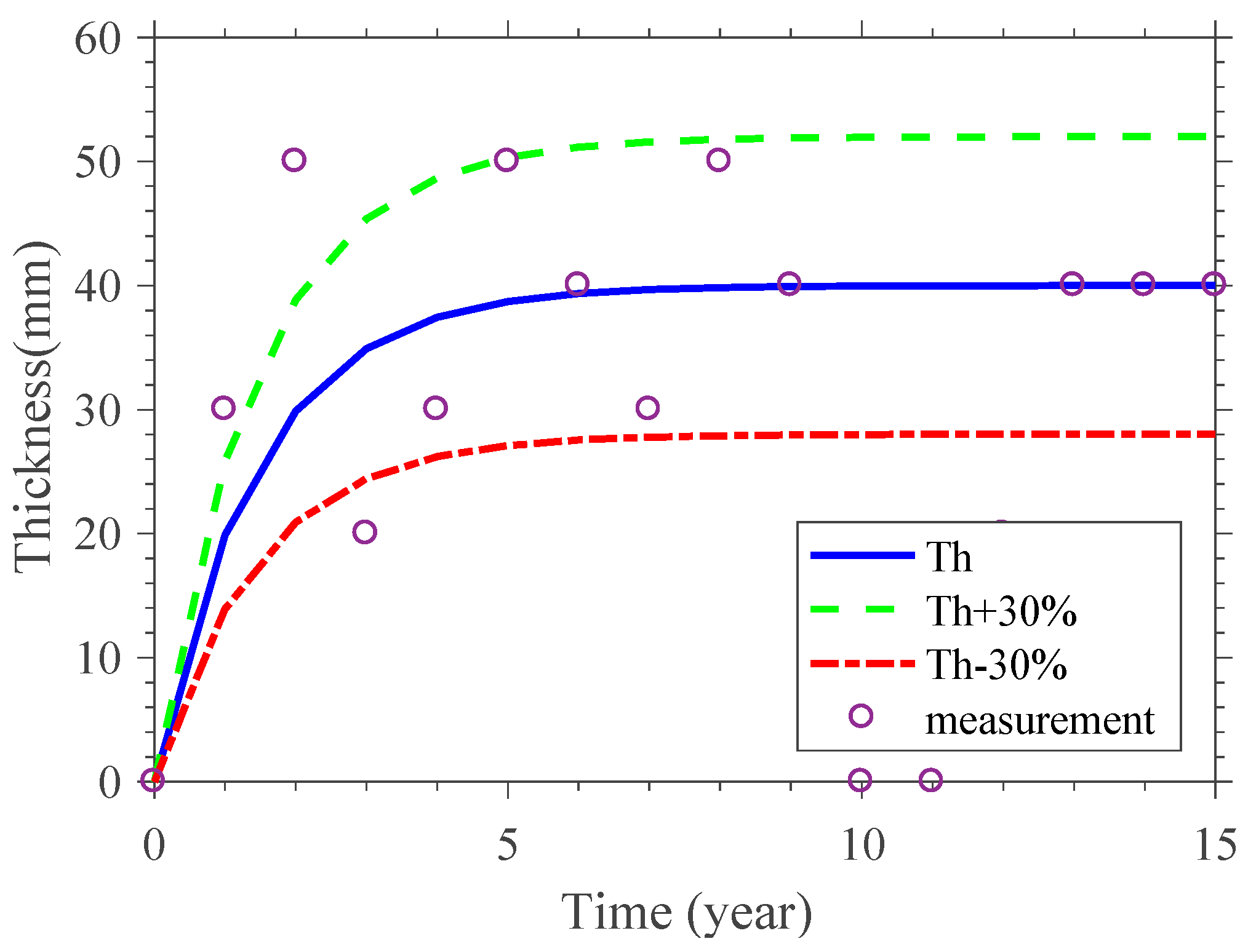
2.1. Modeling of Marine Growth Thickness Stochastic Process
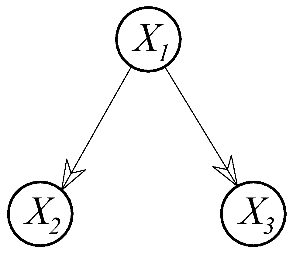
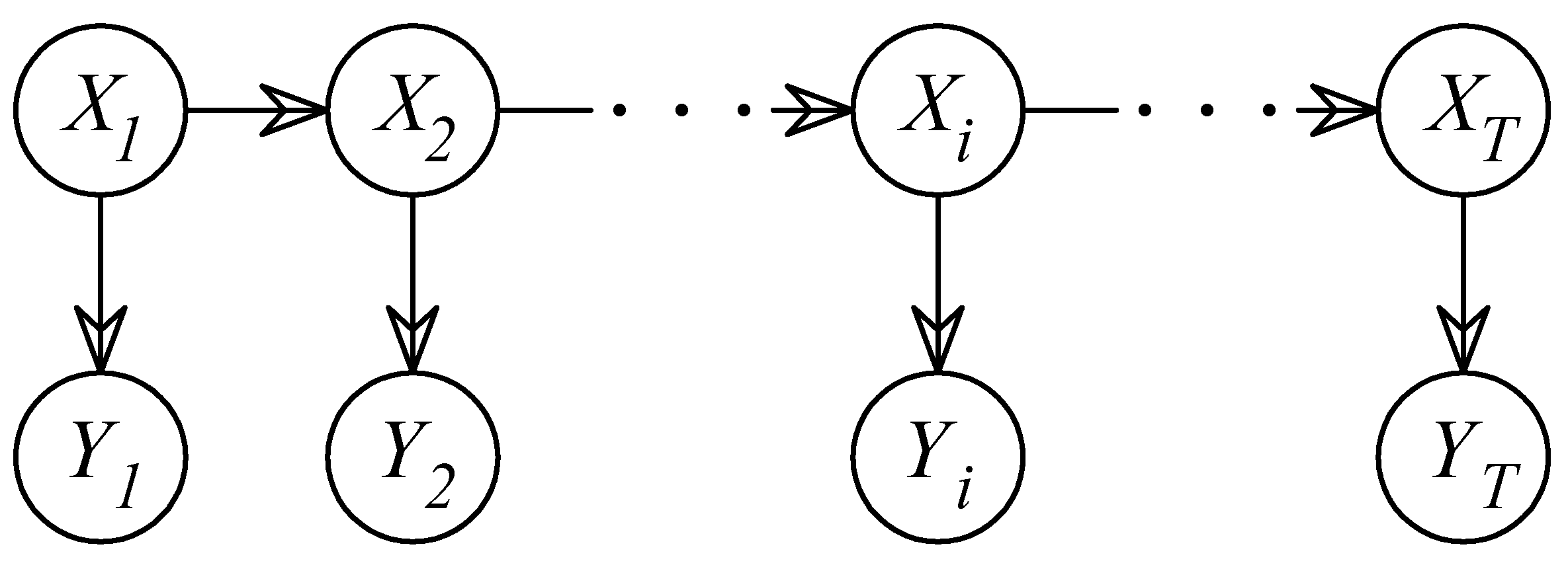
2.2. Dynamic Bayesian Networks for Probability Updating
2.3. DBN for Structural Reliability in the Presence of Marine Growth
3. Results
3.1. Comparison between Two Limit States
3.2. Reliability Updating from One Inspection Time
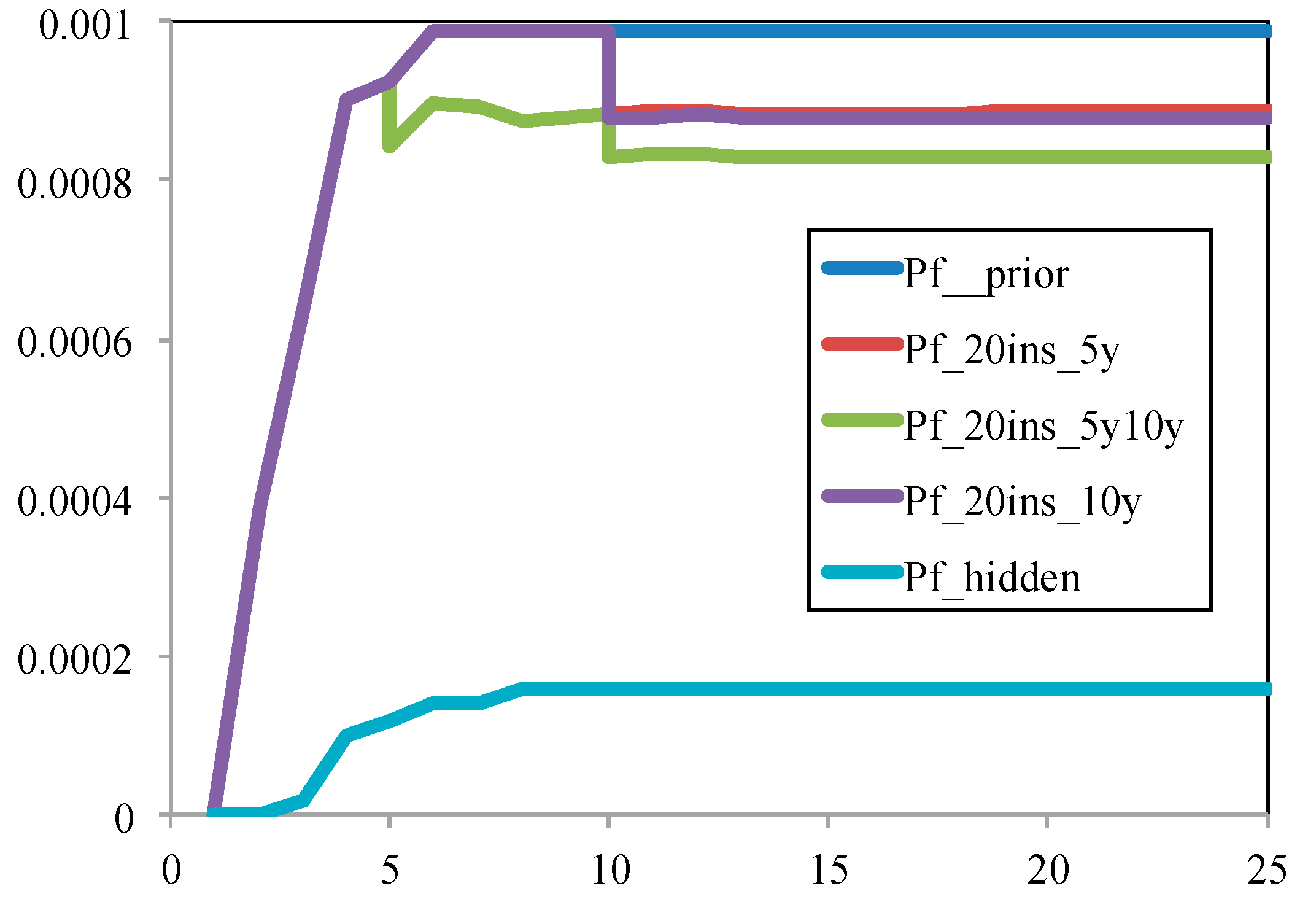
3.3. Reliability Updating from Two Inspection Dates
4. Discussion
5. Conclusions
Author Contributions
Funding
Data Availability Statement
Acknowledgments
Conflicts of Interest
References
- Characklis, W.G.; Marshall, K.C. Microbial fouling and microbial biofouling control. In Biofilms; Characklis, W.G., Marshall, K.C., Eds.; John Wiley and Sons Inc.: New York, NY, USA, 1990; pp. 523–634. [Google Scholar]
- Marty, A.; Schoefs, F.; Soulard, T.; Berhault, C.; Facq, J.-V.; Gaurier, B.; Germain, G. Effect of Roughness of Mussels on Cylinder Forces from a Realistic Shape Modelling. J. Mar. Sci. Eng. 2021, 9, 598. [Google Scholar] [CrossRef]
- Zeinoddini, M.; Bakhtiari, A.; Schoefs, F.; Zandi, A.P. Towards an understanding of marine fouling effects on the vortex-induced vibrations of circular cylinders: Partial coverage issue. Biofouling 2017, 33, 268–280. [Google Scholar] [CrossRef]
- Jusoh, I.; Wolfram, J. Effects of marine growth and hydrodynamic loading on offshore structures. J. Mek. 1996, 1, 77–98. [Google Scholar]
- Schoefs, F.; Boukinda, M.L. Sensitivity Approach for Modeling Stochastic Field of Keulegan–Carpenter and Reynolds Numbers Through a Matrix Response Surface. J. Offshore Mech. Arct. Eng. 2010, 132, 011602. [Google Scholar] [CrossRef]
- Wolfram, J.; Jusoh, I.; Sell, D. Uncertainty in the Estimation of Fluid Loading Due to the Effects of Marine Growth. In Proceedings of the 12th International Conference on Offshore Mechanical and Arctic Engineering (OMAE 1993), Glasgow, Scotland, 20–24 June 1993; Volume 2, pp. 219–228. [Google Scholar]
- Theophanatos, A. Marine Growth and the Hydrodynamic Loading of Offshore Structures. Ph.D. Thesis, University of Srathclyde, Glasgow, UK, 1988. [Google Scholar]
- Mbadinga, M.L.B.; Schoefs, F.; Quiniou-Ramus, V.; Birades, M.; Garretta, R. Marine Growth Colonization Process in Guinea Gulf: Data Analysis. J. Offshore Mech. Arct. Eng. 2007, 129, 97–106. [Google Scholar] [CrossRef]
- Ameryoun, H.; Schoefs, F.; Barillé, L.; Thomas, Y. Stochastic Modeling of Forces on Jacket-Type Offshore Structures Colonized by Marine Growth. J. Mar. Sci. Eng. 2019, 7, 158. [Google Scholar] [CrossRef]
- Schoefs, F.; Ameryoun, A. On-site test of components and sensors exposed to marine degradations processes: Fatigue, corrosion and biofouling. In Proceedings of the 3rd Offshore Wind R&D Conference, Topic Test Facilities & Demonstration Sites, Atlantic Sail City Hotel, Bremerhaven, Germany, 14–16 November 2018; Available online: https://www.rave-offshore.de/en/conference-2018.html (accessed on 29 December 2021).
- Quillien, N.; Ameryoun, H.; Barillier, A.; Berhault, C.; Boukerma, K.; Bressy, C.; Briand, J.F.; Cayocca, K.; Compère, C.; Damblans, G.; et al. Biofouling: The need to develop interdiscisplinary teamwork skills for MRE. In Proceedings of the International Conference on Ocean Energy (ICOE 2018), Session Underwater Technologies Getting Wet, Corroded and Colonized, La Cité de la Mer, Cherbourg, France, 12–14 June 2018. [Google Scholar]
- Bakhtiari, A.; Schoefs, F.; Ameryoun, H. Unified Approach For Estimating Of The Drag Coefficient In Offshore Structures In Presence Of Bio-Colonization. In Proceedings of the 37th International Conference on Offshore Mechanics and Arctic Engineering (O.M.A.E.’ 18), Madrid, Spain, 17–22 June 2018. [Google Scholar]
- Schoefs, F.; Bakhtiari, A.; Hameryoun, H.; Quillien, N.; Damblans, G.; Reynaud, M.; Berhault, C.; O’Byrne, M. Assessing and modeling the thickness and roughness of marine growth for load computation on mooring lines. In Proceedings of the Floating Offshore Wind Turbine Conference (FOWT 2019), Session Friday Morning ‘Wind Energy Devices I’, Le Corum, Montpellier, France, 24–26 April 2019. [Google Scholar]
- Schoefs, F.; O’Byrne, M.; Pakrashi, V.; Gosh, B.; Oumouni, M.; Soulard, T.; Reynaud, M. Fractal Dimension as an Effective Feature for Characterizing Hard Marine Growth Roughness from Underwater Image Processing in Controlled and Uncontrolled Image Environments. J. Mar. Sci. Eng. 2021, 9, 1344. [Google Scholar] [CrossRef]
- Marty, A.; Berhault, C.; Damblans, G.; Facq, J.-V.; Gaurier, B.; Germain, G.; Soulard, T.; Schoefs, F. Experimental study of hard marine growth effect on the hydrodynamical behaviour of a submarine cable. Appl. Ocean Res. 2021, 114, 102810. [Google Scholar] [CrossRef]
- Quillien, N.; Damblans, G.; Boukerma, K.; Briand, J.F.; Bressy, C.; Carlier, A.; Compère, C.; Dreanno, C.; Jacob, D.; Leblanc, V.; et al. Why and how characterizing biofouling for FOWT? In Proceedings of the Floating Offshore Wind Turbine Conference (FOWT 2019), Session Friday Afternoon ‘Resource and Environmental Impact’, Le Corum, Montpellier, France, 24–26 April 2019. [Google Scholar]
- Schoefs, F.; Chapeleau, X.; Lupi, C. Statistical analysis of Mooring loading of a buoy through FOS and use in risk analysis. In Proceedings of the 54th ESReDA Seminar on Risk, Reliability and Safety of Energy Systems in Coastal and Marine Environments, Université de Nantes, Sea and Litoral Research Institute, MSH Ange Guepin, Nantes, France, 25–26 April 2018. [Google Scholar]
- O’Byrne, M.; Schoefs, F.; Pakrashi, V.; Ghosh, B. An underwater lighting and turbidity image repository for analysing the performance of image-based non-destructive techniques. Struct. Infrastruct. Eng. 2017, 14, 104–123. [Google Scholar] [CrossRef]
- O’Byrne, M.; Pakrashi, V.; Schoefs, F.; Ghosh, B. A Stereo-Matching Technique for Recovering 3D Information from Underwater Inspection Imagery. Comput. Civ. Infrastruct. Eng. 2018, 33, 193–208. [Google Scholar] [CrossRef]
- O’Byrne, M.; Pakrashi, V.; Schoefs, F.; Ghosh, B. Semantic Segmentation of Underwater Imagery Using Deep Networks Trained on Synthetic Imagery. J. Mar. Sci. Eng. 2018, 6, 93. [Google Scholar] [CrossRef]
- Faber, M.H.; Hansen, P.F.; Jepsen, F.D.; Mo/ller, H.H. Reliability-Based Management of Marine Fouling. J. Offshore Mech. Arct. Eng. 2001, 123, 76–83. [Google Scholar] [CrossRef]
- Rouhan, A.; Schoefs, F. Probabilistic modeling of inspection results for offshore structures. Struct. Saf. 2003, 25, 379–399. [Google Scholar] [CrossRef]
- Morison, J.R.; Johnson, J.W.; Schaaf, S.A. The Force Exerted by Surface Waves on Piles. J. Pet. Technol. 1950, 2, 149–154. [Google Scholar] [CrossRef]
- Yan, T.; Yan, W.; Dong, Y.; Wang, H.; Yan, Y.; Liang, G. Marine fouling of offshore installations in the northern Beibu Gulf of China. Int. Biodeterior. Biodegrad. 2006, 58, 99–105. [Google Scholar] [CrossRef]
- Henry, P.-Y.; Nedrebø, E.L.; Myrhaug, D. Visualisation of the effect of different types of marine growth on cylinders’ wake structure in low Re steady flows. Ocean Eng. 2016, 115, 182–188. [Google Scholar] [CrossRef]
- Shi, W.; Park, H.-C.; Baek, J.-H.; Kim, C.-W.; Kim, Y.-C.; Shin, H.-K. Study on the marine growth effect on the dynamic response of offshore wind turbines. Int. J. Precis. Eng. Manuf. 2012, 13, 1167–1176. [Google Scholar] [CrossRef]
- Dürr, S.; Thomason, J.C. Biofouling; Wiley-Blackwell: New York, NY, USA, 2009; Available online: http://eu.wiley.com/WileyCDA/WileyTitle/productCd-1405169265.html (accessed on 29 December 2021).
- API RP 2A WSD. Recommended Practice for Planning, Designing, and Constructing Fixed Offshore Platforms, 21st ed.; API Publications Department: Washington, District of Columbia, United States, 2005; Volume 2. [Google Scholar]
- Sarpkaya, T. On the Effect of Roughness on Cylinders. J. Offshore Mech. Arct. Eng. 1990, 112, 334–340. [Google Scholar] [CrossRef]
- Buresti, G. The effect of surface roughness on the flow regime around circular cylinders. J. Wind. Eng. Ind. Aerodyn. 1981, 8, 105–114. [Google Scholar] [CrossRef]
- Batham, J.P. Pressure distributions on circular cylinders at critical Reynolds numbers. J. Fluid Mech. 1973, 57, 209–228. [Google Scholar] [CrossRef]
- Güven, O.; Farell, C.; Patel, V.C. Surface-roughness effects on the mean flow past circular cylinders. J. Fluid Mech. 1980, 98, 673–701. [Google Scholar] [CrossRef]
- Ribeiro, J.D. Effects of surface roughness on the two-dimensional flow past circular cylinders I: Mean forces and pressures. J. Wind. Eng. Ind. Aerodyn. 1991, 37, 299–309. [Google Scholar] [CrossRef]
- Ribeiro, J.D. Effects of surface roughness on the two-dimensional flow past circular cylinders II: Fluctuating forces and pressures. J. Wind. Eng. Ind. Aerodyn. 1991, 37, 311–326. [Google Scholar] [CrossRef]
- Zhou, B.; Wang, X.; Gho, W.M.; Tan, S.K. Force and flow characteristics of a circular cylinder with uniform surface roughness at subcritical Reynolds numbers. Appl. Ocean Res. 2015, 49, 20–26. [Google Scholar] [CrossRef]
- Callow, M.E.; Callow, J.A. Marine biofouling: A sticky problem. Biologist 2002, 49, 1–5. [Google Scholar]
- Railkin, A.I. Marine Biofouling: Colonization Processes and Defenses; CRC Press: Boca Raton, FL, USA, 2003. [Google Scholar]
- Handå, A.; Alver, M.; Edvardsen, C.V.; Halstensen, S.; Olsen, A.J.; Øie, G.; Reitan, K.I.; Olsen, Y.; Reinertsen, H. Growth of farmed blue mussels (Mytilus edulis L.) in a Norwegian coastal area; Comparison of food proxies by DEB modeling. J. Sea Res. 2011, 66, 297–307. [Google Scholar] [CrossRef]
- Heaf, N.J. The Effect of Marine Growth on the Performance of Fixed Offshore Platforms in the North Sea. In Proceedings of the Offshore Technology Conference, Houston, TX, USA, 30 April–3 May 1979; p. 14. [Google Scholar] [CrossRef]
- Bayne, B.L. Growth and the delay of metamorphosis of the larvae of Mytilus edulis (L.). Ophelia 1965, 2, 1–47. [Google Scholar] [CrossRef]
- Bayne, B.L.; Worrall, C.M. Growth and Production of Mussels Mytilus edulis from Two Populations. Mar. Ecol. Prog. Ser. 1980, 3, 317–328. [Google Scholar] [CrossRef]
- Gompertz, B., XXIV. On the nature of the function expressive of the law of human mortality, and on a new mode of determining the value of life contingencies. In a letter to Francis Baily, Esq. FRS &c. Philos. Trans. R. Soc. Lond. 1825, 115, 513–583. [Google Scholar] [CrossRef]
- von Bertalanffy, L. Quantitative Laws in Metabolism and Growth. Q. Rev. Biol. 1957, 32, 217–231. [Google Scholar] [CrossRef]
- Vincenzi, S.; Jesensek, D.; Crivelli, A.J. Biological and statistical interpretation of size-at-age, mixed-effects models of growth. R. Soc. Open Sci. 2020, 7, 192146. [Google Scholar] [CrossRef] [PubMed]
- Barillé Boyer, A.-L. Contribution à l’étude des potentialités conchylicoles du Pertuis Breton. Ph.D. Thesis, Université d’aix Marseille, Marseille, France, 1996. (In French). [Google Scholar]
- Veritec. Marine Growth Data Bank-Volume 3; Final report of JIP “MAGDA”, Internal Report of Veritec; Veritec: Minneapolis, MN, USA, 1987. [Google Scholar]
- van der Stap, T.; Coolen, J.W.P.; Lindeboom, H.J. Data from: Marine fouling assemblages on offshore gas platforms in the southern North Sea: Effects of depth and distance from shore on biodiversity. PLoS ONE 2016, 11, e0146324. [Google Scholar] [CrossRef]
- Decurey, B.; Schoefs, F.; Barillé, A.-L.; Soulard, T. Model of Bio-Colonisation on Mooring Lines: Updating Strategy Based on a Static Qualifying Sea State for Floating Wind Turbines. J. Mar. Sci. Eng. 2020, 8, 108. [Google Scholar] [CrossRef]
- Komušanac, I. Wind Energy in Europe in 2019: Trends and Statistics. On Line Resource. Published in February 2020. Available online: https://windeurope.org (accessed on 29 December 2021).
- Maar, M.; Bolding, K.; Petersen, J.K.; Hansen, J.L.; Timmermann, K. Local effects of blue mussels around turbine foundations in an ecosystem model of Nysted off-shore wind farm, Denmark. J. Sea Res. 2009, 62, 159–174. [Google Scholar] [CrossRef]
- Bruijs, M.C.M. Biological Fouling Survey of Marine Fouling on Turbine Support Structures of the Offshore784Windfarm Egmond aan Zee; Report prepared for Noordzeewind; 50863511-TOS/PCW 10-4207,785 OWEZ_R_112_T1_20100226; KEMA Nederland B.V.: Arnhem, The Netherlands, 2010. [Google Scholar]
- Schoefs, F. Sensitivity approach for modelling the environmental loading of marine structures through a matrix response surface. Reliab. Eng. Syst. Saf. 2008, 93, 1004–1017. [Google Scholar] [CrossRef][Green Version]
- Picken, G.B. Review of marine fouling organisms in the North Sea on offshore structures. In Discussion Forum and Exhibition on Offshore Engineering with Elastomers; Plastics and Rubber Inst.: London, UK, 1985; Volume 5, pp. 5.1–5.10. [Google Scholar]
- El Hajj, B.; Schoefs, F.; Castanier, B.; Yeung, T. A condition-based deterioration model for the stochastic dependency of corrosion rate and crack propagation in a submerged concrete structure. Comput. Aided Civ. Infrastruct. Eng. 2016, 32, 18–33. [Google Scholar] [CrossRef]
- Nerzic, R.; Frelin, C.; Prevosto, M.; Quiniou-Ramus, V. Joint Distributions for Wind/waves/current in West Africa and derivation of Multi Variate Extreme I-FORM Contours. In Proceedings of the 17th International Offshore and Polar Engineering Conference, Lisbon, Portugal, 1–6 July 2007; pp. 81–88. [Google Scholar]
- Straub, D. Stochastic Modeling of Deterioration Processes through Dynamic Bayesian Networks. J. Eng. Mech. 2009, 135, 1089–1099. [Google Scholar] [CrossRef]


| Inspection Time from Installation of Structures (Years) | ||||||||||||||||
|---|---|---|---|---|---|---|---|---|---|---|---|---|---|---|---|---|
| 0 | 1 | 2 | 3 | 4 | 5 | 6 | 7 | 8 | 9 | 10 | 11 | 12 | 13 | 14 | 15 | |
| Field Measurement (mm)Measurement (mm) | 30 | 20 | 20 | 30 | 20 | 10 | 20 | 50 | 40 | 20 | 20 | 10 | 40 | |||
| 30 | 70 | 10 | 20 | 40 | 30 | 10 | 20 | 40 | 40 | 40 | ||||||
| 50 | 20 | 80 | 30 | 20 | 20 | 20 | 20 | 30 | ||||||||
| 10 | 10 | |||||||||||||||
| 10 | 20 | |||||||||||||||
| 20 | 30 | |||||||||||||||
| 5 | ||||||||||||||||
| 20 | ||||||||||||||||
| 30 | ||||||||||||||||
| Type | Parameter (Unit) | Description | Value |
|---|---|---|---|
| Geometry and material | D (m) | Diameter | 0.3 |
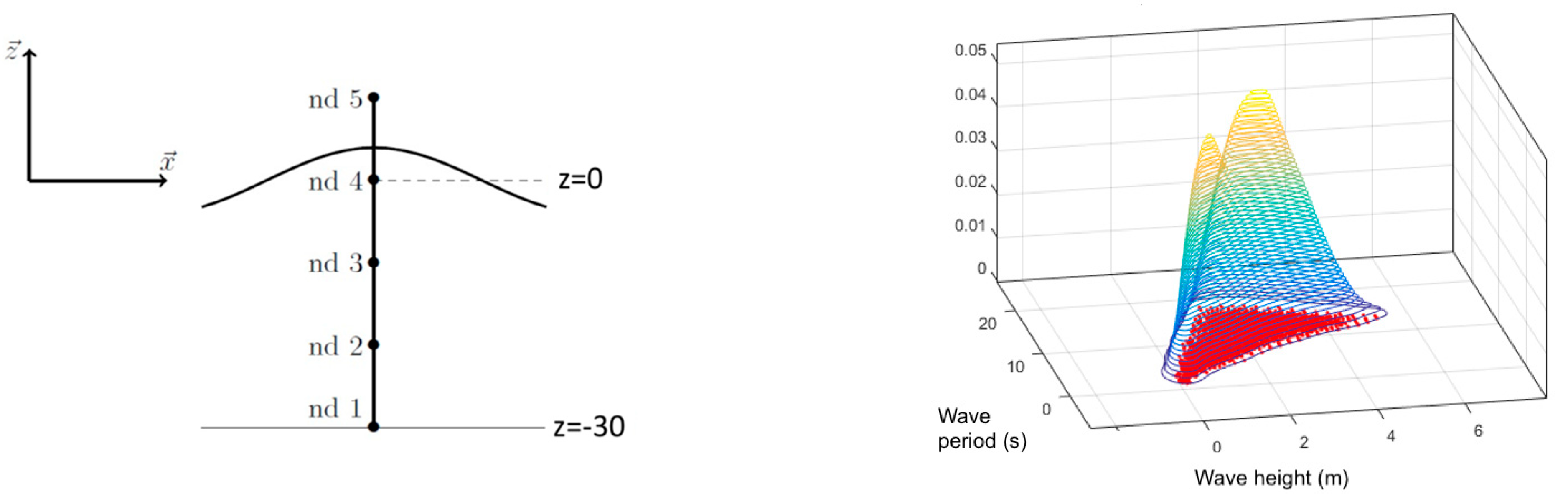
| d (m) | Water depth (utile length of the monopile) | 30 | |
| e (m) | Thickness | 0.025 | |
| E (Pa) | Young’s modulus | 2.1 × 10¹¹ | |
| G (Pa) | Shear modulus | 8.0769 × 10¹⁰ | |
| ρ (kg/m3) | Density | 7800 | |
| σe (Pa) | Yield stress | 2 × 10⁸ | |
| Environment | H and T | See [9] | |
| Marine growth | α | N(μ = 0.04; COV = 0.3) | |
| β | 0.6875 | ||
| Layer 1 | From 0 (m) to −5 (m) | Th1 = Th | |
| Layer 2 Layer 3 | From −5 (m) to −19 (m) From −10 (m) to bottom (m) | Th2 = 0.5 × Th Th3 = 0 × Th |
| Nodes | Prior Distribution | Number of States | Boundaries |
|---|---|---|---|
| N(μ = 0.04; COV = 0.3) | 10 | [0; 0.4] | |
| - | 40 | [0; 0.4] | |
| - | 40 | [0; 3] × 108 | |
| - | Binary | - |
| Errors Relative to Mean Pf | |||||||||
|---|---|---|---|---|---|---|---|---|---|
| No of Measurement | 3 | 5 | 10 | 15 | 20 | 30 | 50 | 70 | 100 |
| 5% quantiles | 16% | 14% | 9% | 7% | 6% | 5% | 4% | 3% | 2% |
| 95% quantiles | 14% | 12% | 7% | 6% | 6% | 4% | 4% | 3% | 2% |
| Case | Number of Measurements | |
|---|---|---|
| 5 Years | 10 Years | |
| 1 | 20 | 0 |
| 2 | 10 | 10 |
| 3 | 0 | 20 |
Publisher’s Note: MDPI stays neutral with regard to jurisdictional claims in published maps and institutional affiliations. |
© 2022 by the authors. Licensee MDPI, Basel, Switzerland. This article is an open access article distributed under the terms and conditions of the Creative Commons Attribution (CC BY) license (https://creativecommons.org/licenses/by/4.0/).
Share and Cite
Schoefs, F.; Tran, T.-B. Reliability Updating of Offshore Structures Subjected to Marine Growth. Energies 2022, 15, 414. https://doi.org/10.3390/en15020414
Schoefs F, Tran T-B. Reliability Updating of Offshore Structures Subjected to Marine Growth. Energies. 2022; 15(2):414. https://doi.org/10.3390/en15020414
Chicago/Turabian StyleSchoefs, Franck, and Thanh-Binh Tran. 2022. "Reliability Updating of Offshore Structures Subjected to Marine Growth" Energies 15, no. 2: 414. https://doi.org/10.3390/en15020414
APA StyleSchoefs, F., & Tran, T.-B. (2022). Reliability Updating of Offshore Structures Subjected to Marine Growth. Energies, 15(2), 414. https://doi.org/10.3390/en15020414