
Fuzzy Adaptive Type II Controller for Two-Mass System


Abstract
:1. Introduction
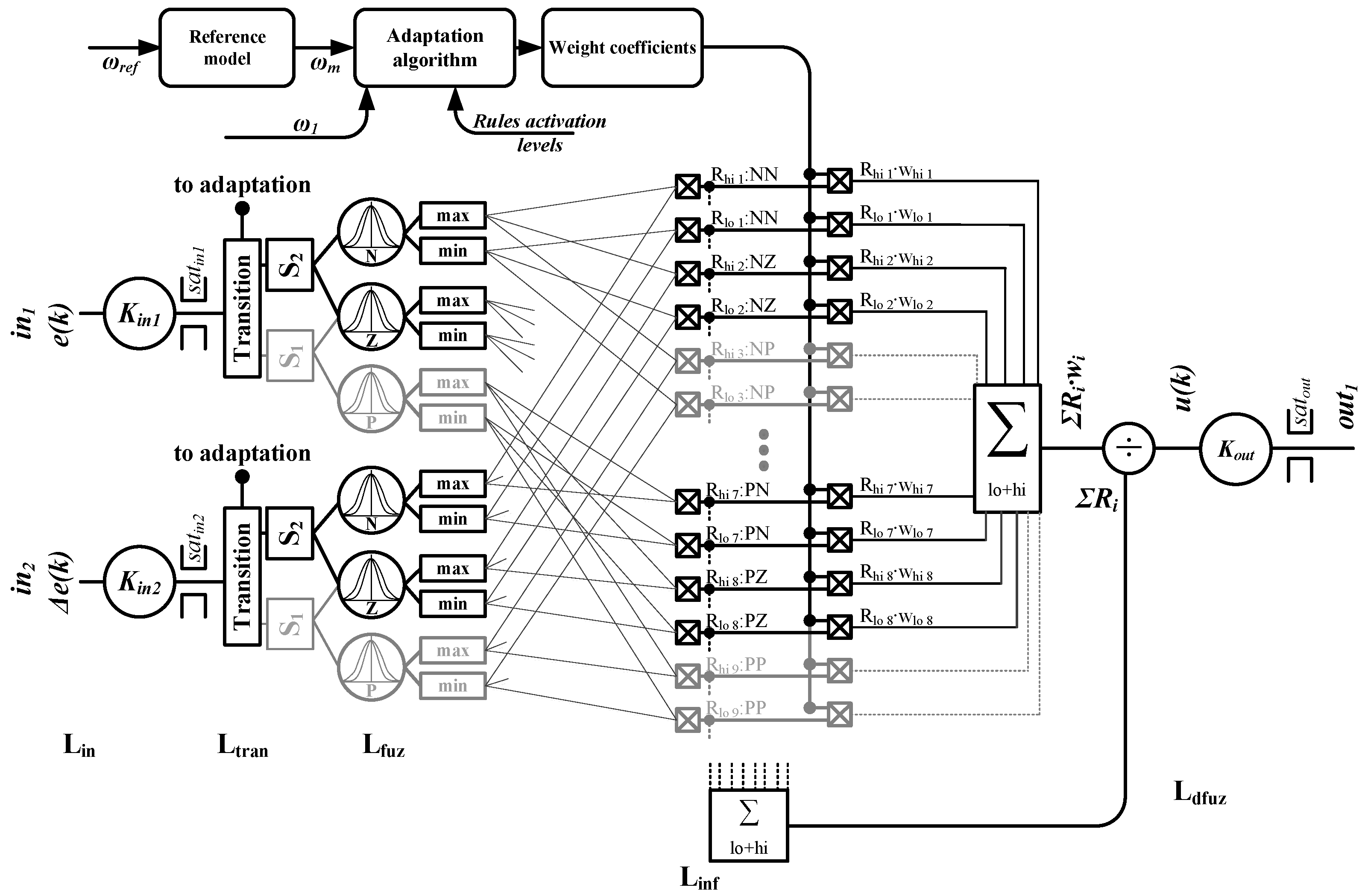
2. Adaptive Neuro-Fuzzy Controller with Petri Transition Layer
2.1. Input Layer
2.2. Transition Petri Layer
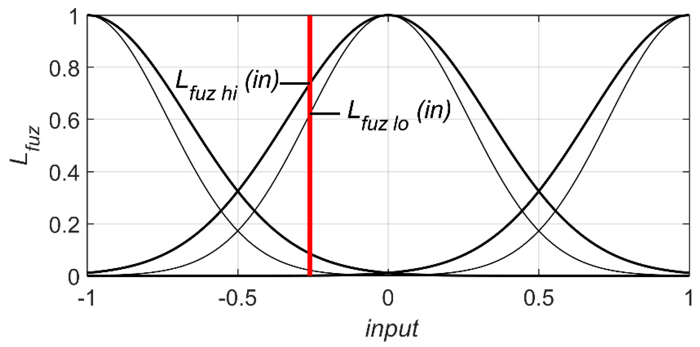
2.3. Fuzzyfication Layer
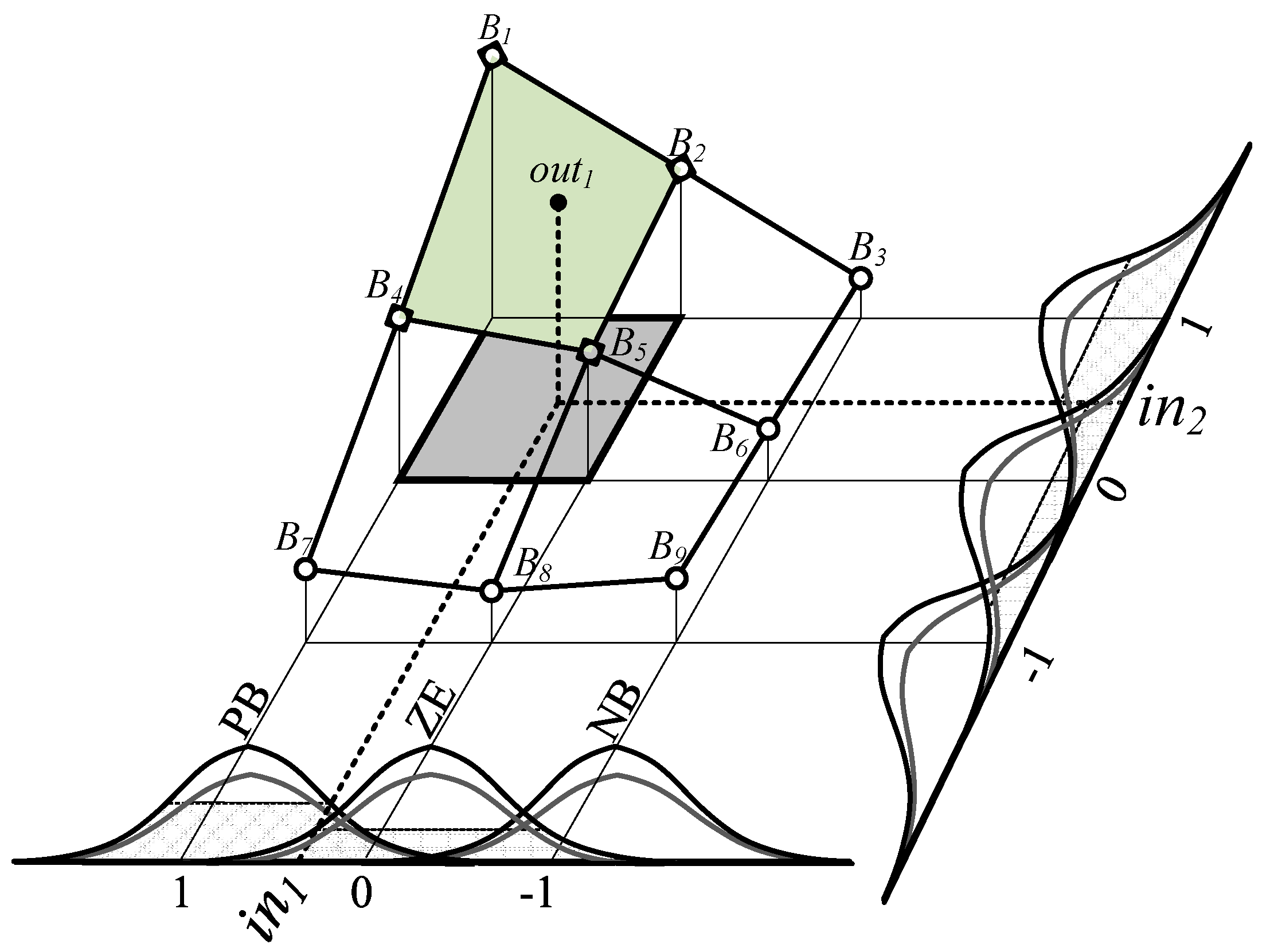
2.4. Inference Layer
2.5. Defuzyfication Layer
2.6. Adaptation Algorithm
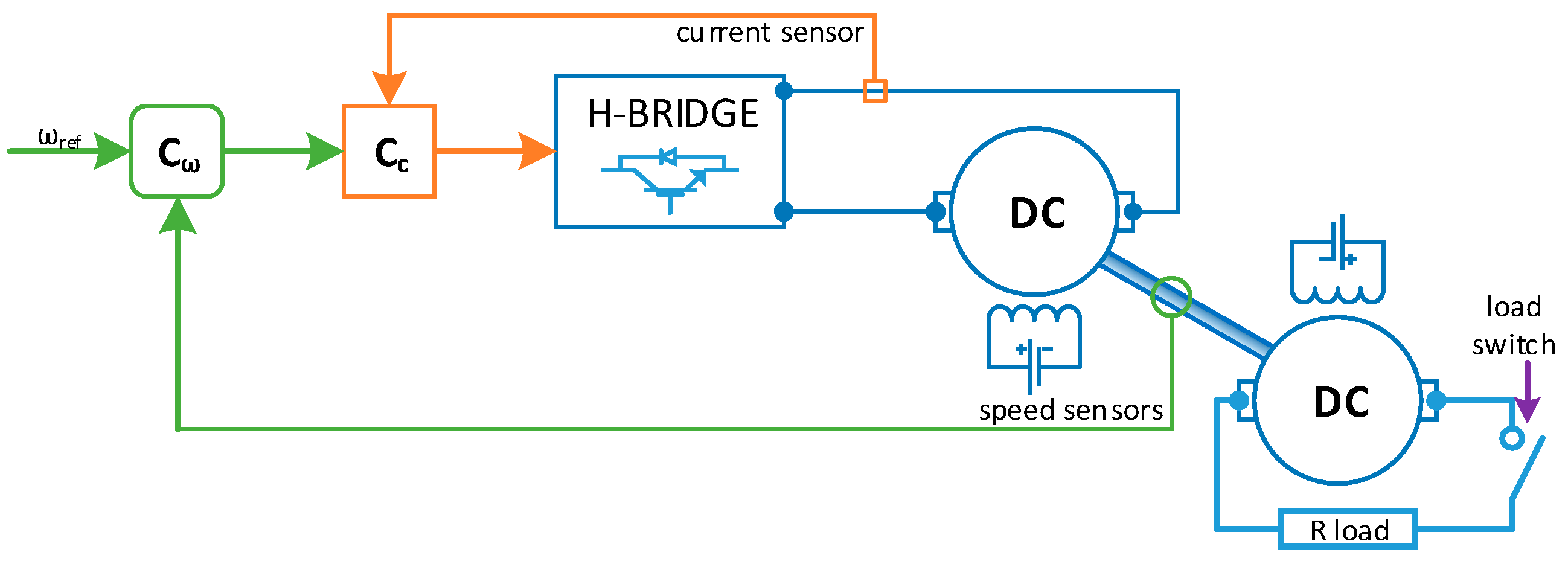
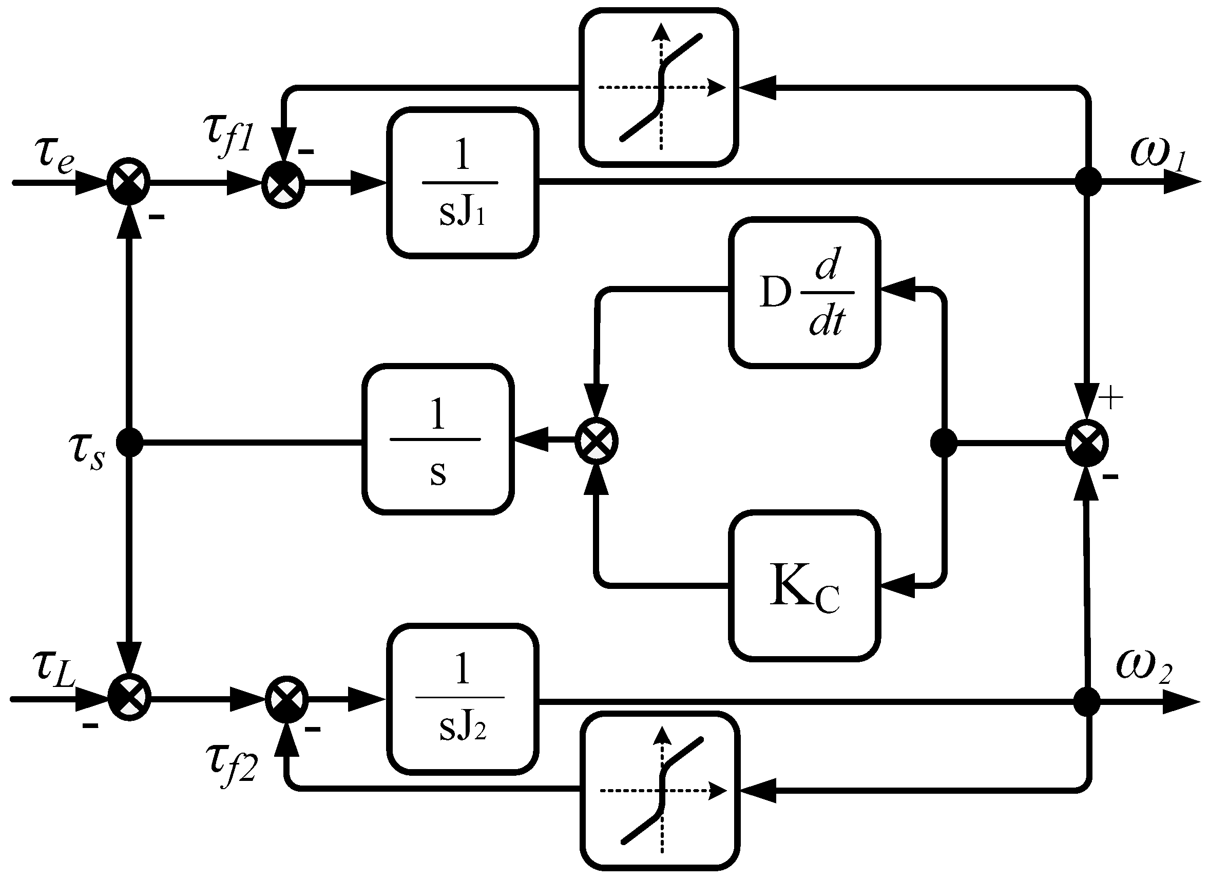
3. Two Mass System—SimPowerSystem Model
4. Simulations
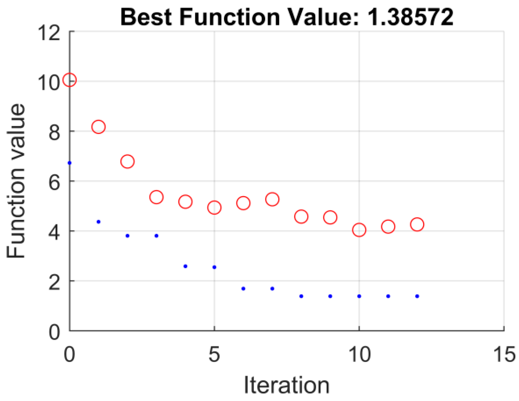
4.1. Optimization Process
4.2. The Cost Functions for Optimization
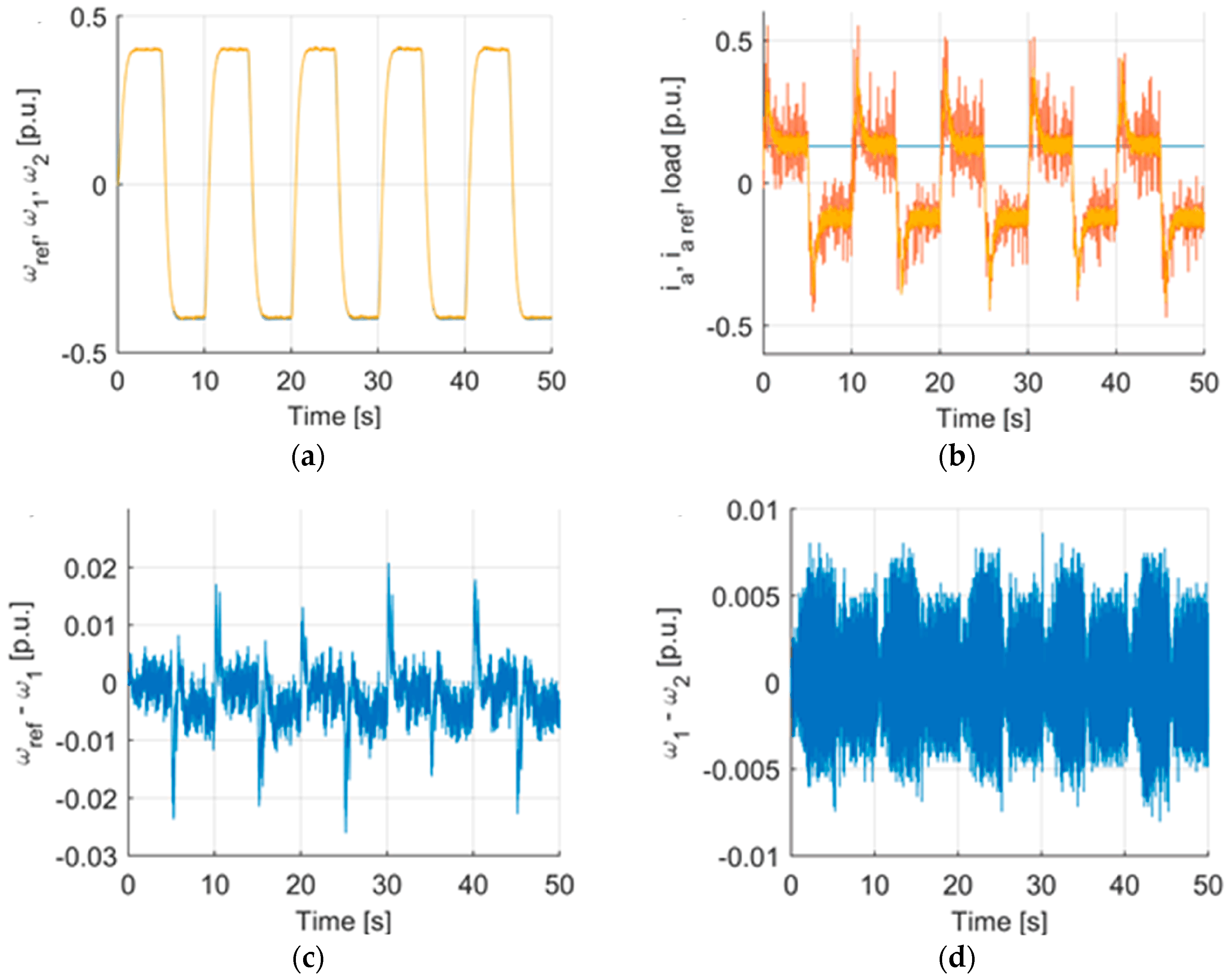
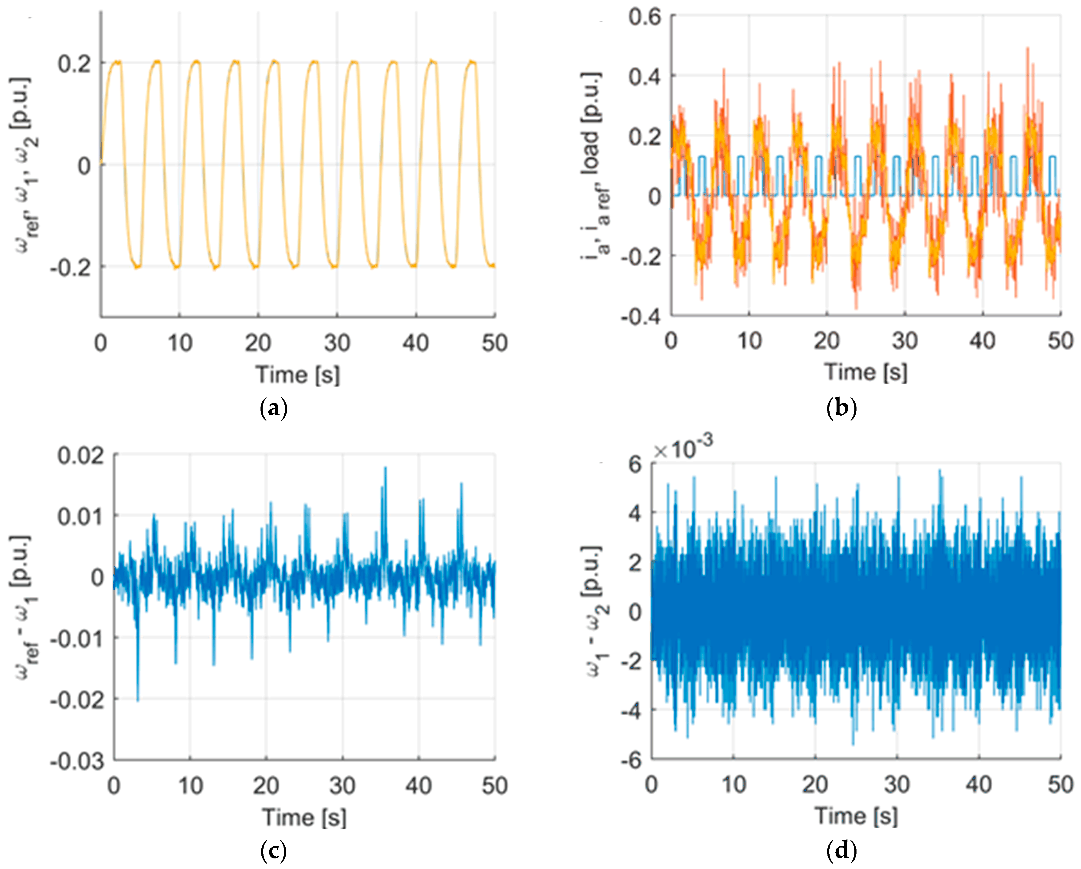
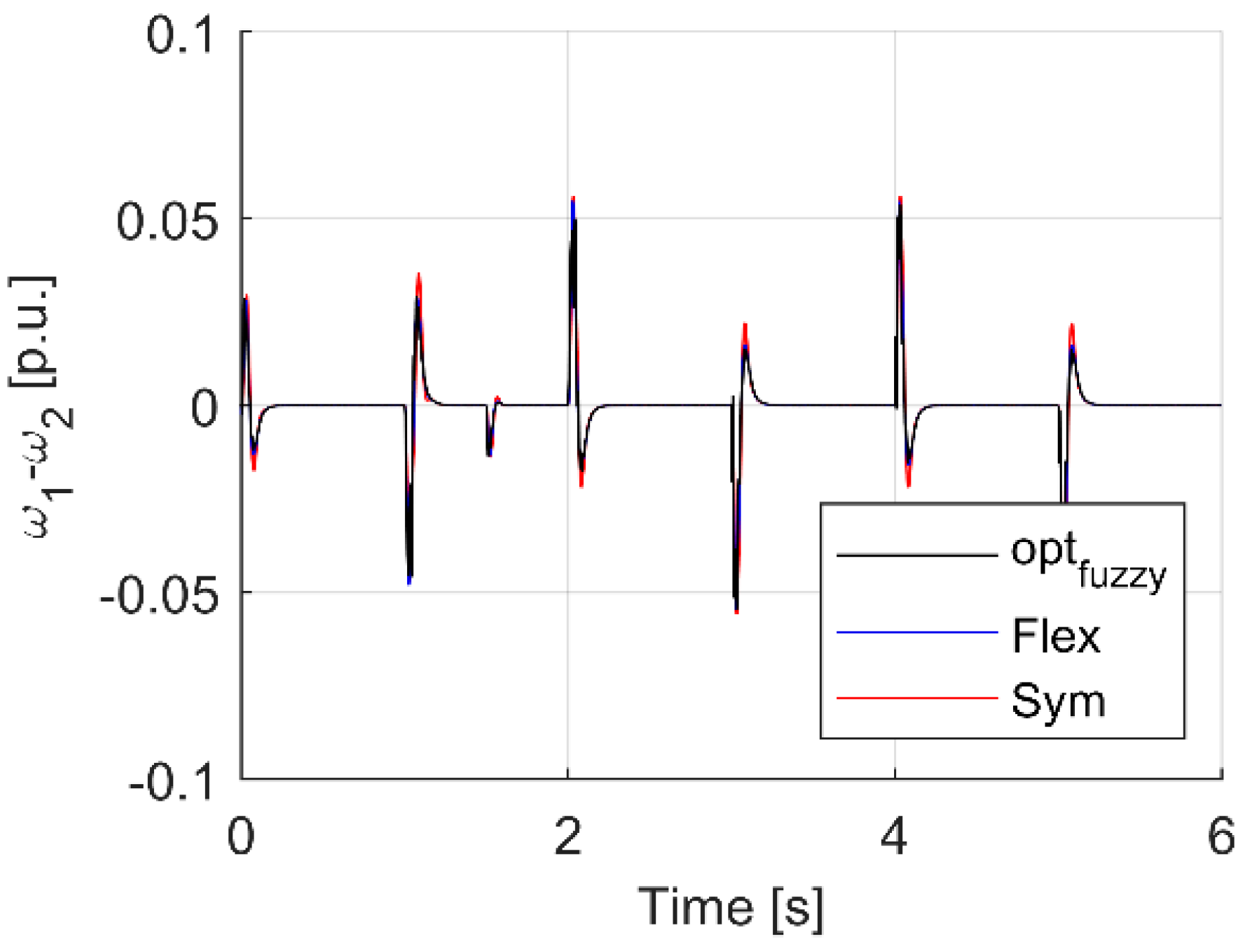
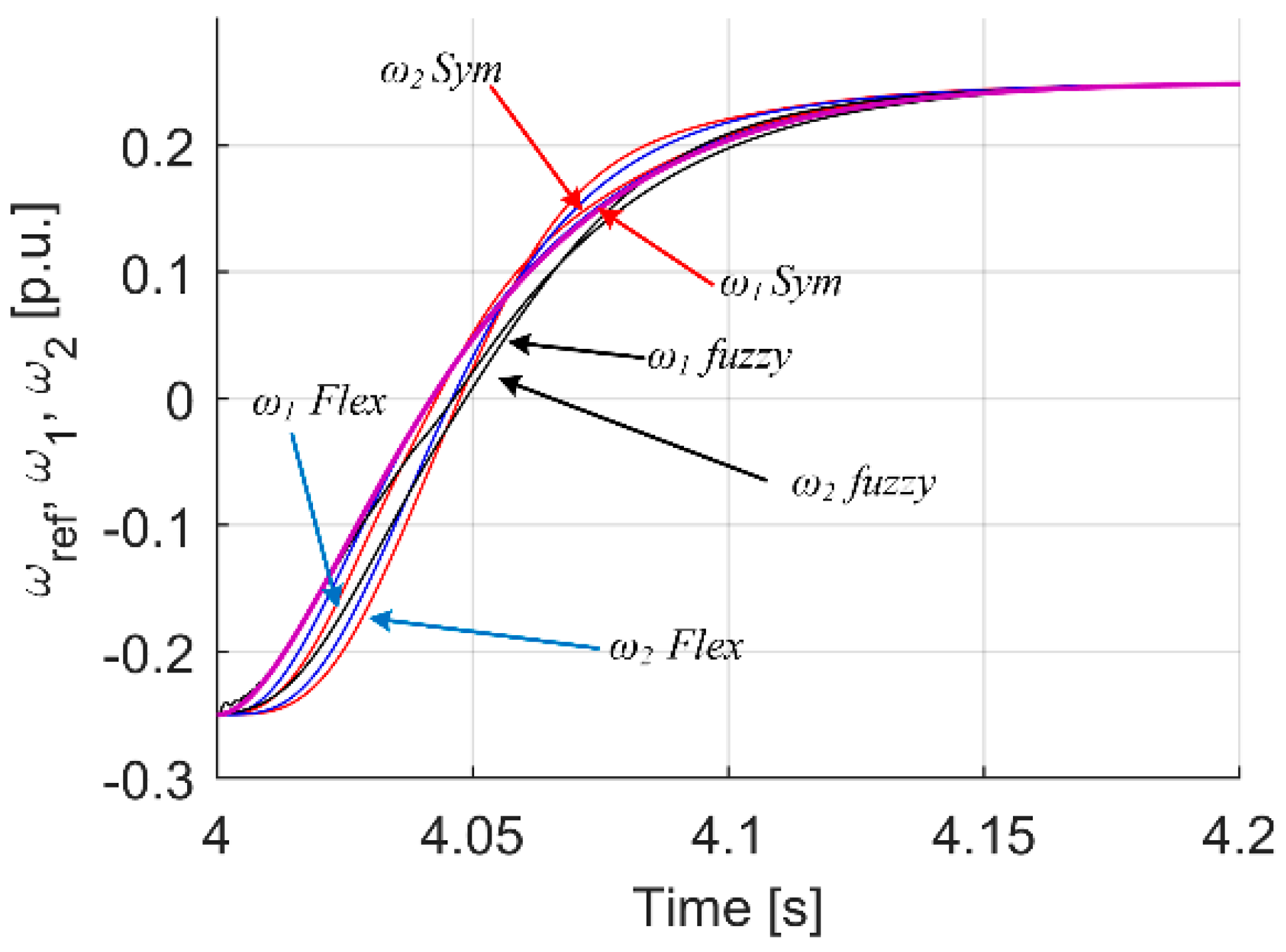
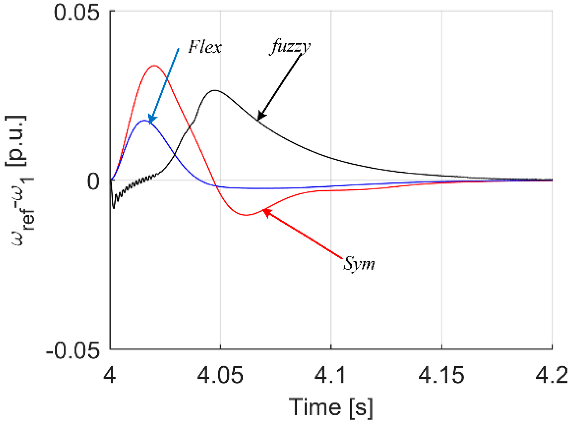
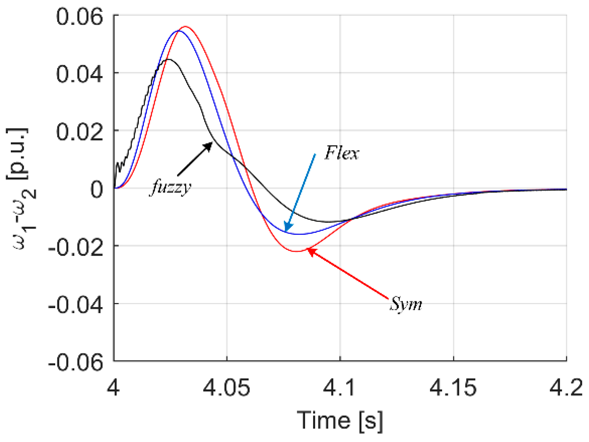
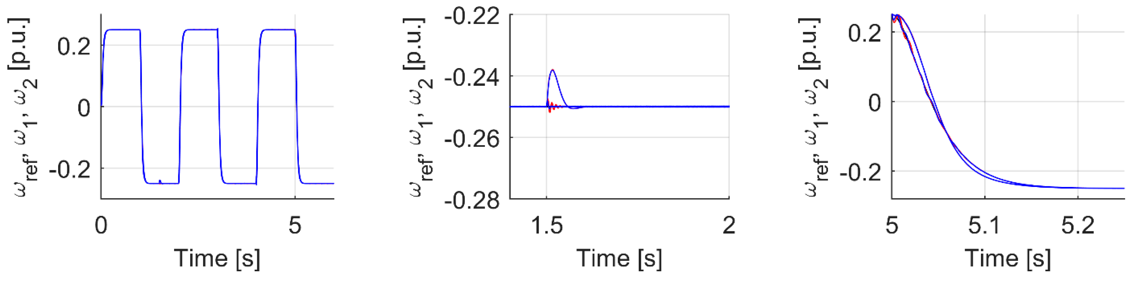
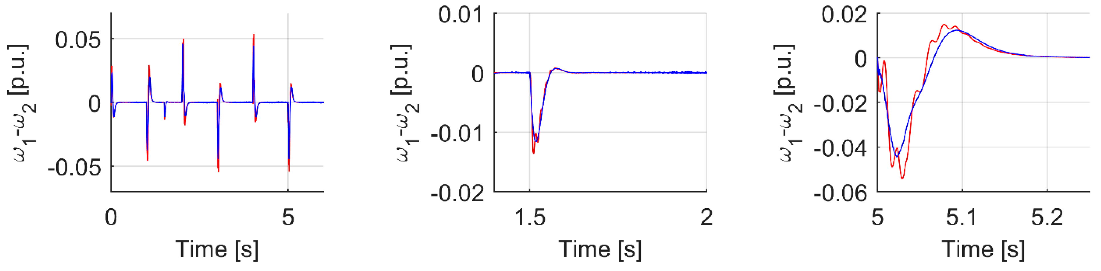
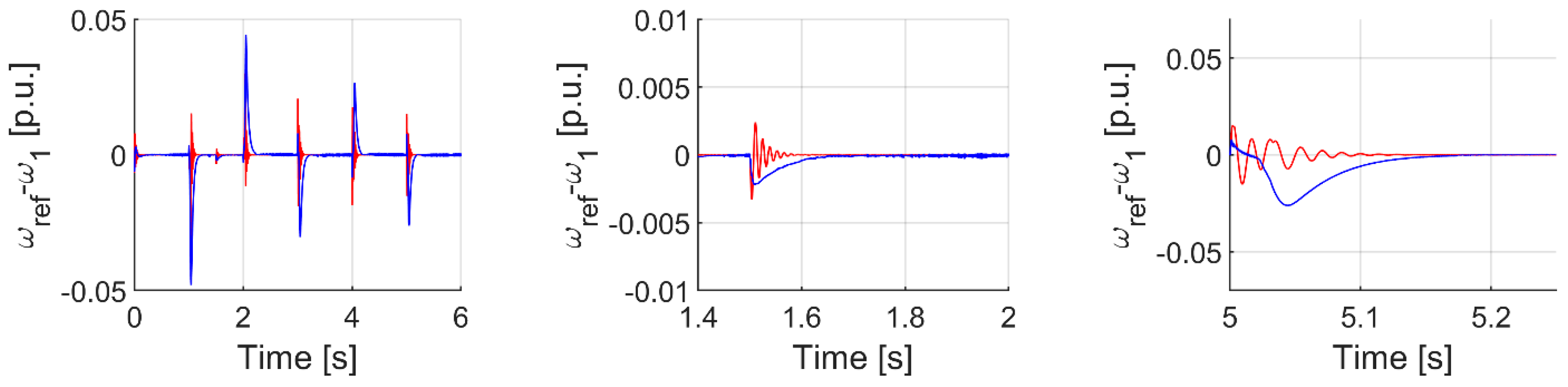
4.3. Simulation Transients
4.4. Adaptive Fuzzy Controller with Type I Fuzzy Sets
4.5. Adaptive Fuzzy Controller with Type II Fuzzy Sets and Petri Transition Layer
5. Experimental Verification
6. Conclusions
Author Contributions
Funding
Conflicts of Interest
References
- Ohnishi, K.; Katsura, S.; Shimono, T. Motion control for real-world haptics. IEEE Ind. Electron. Mag. 2010, 4, 16–19. [Google Scholar] [CrossRef]
- Inoue, Y.; Katsura, S. Spatial disturbance suppression of a flexible system based on wave model. IEEJ J. Ind. Appl. 2018, 7, 236–243. [Google Scholar] [CrossRef] [Green Version]
- Łuczak, D. Nonlinear Identification with Constraints in Frequency Domain of Electric Direct Drive with Multi-Resonant Mechanical Part. Energies 2021, 14, 7190. [Google Scholar] [CrossRef]
- Li, P.; Wang, L.; Zhong, B.; Zhang, M. Linear Active Disturbance Rejection Control for Two-mass Systems via Singular Perturbation Approach. IEEE Ind. Inform. 2021; in press. [Google Scholar] [CrossRef]
- Lozynskyy, A.; Chaban, A.; Perzyński, T.; Szafraniec, A.; Kasha, L. Application of Fractional-Order Calculus to Improve the Mathematical Model of a Two-Mass System with a Long Shaft. Energies 2021, 14, 1854. [Google Scholar] [CrossRef]
- Zhang, G.; Furusho, J. Speed control of two—Inertia system by PI/PID control. IEEE Trans. Ind. Electron. 2000, 47, 603–609. [Google Scholar] [CrossRef]
- Goubej, M. Fundamental performance limitations in PID controlled elastic two-mass systems. In Proceedings of the IEEE International Conference on Advanced Intelligent Mechatronics (AIM), Banff, AB, Canada, 12–15 July 2016; pp. 828–833. [Google Scholar]
- Li, X.; Shang, D.; Li, H.; Li, F. Resonant Suppression Method Based on PI control for Serial Manipulator Servo Drive System. Sci. Prog. 2020, 103, 1–39. [Google Scholar] [CrossRef]
- Nalepa, R.; Najdek, K.; Wróbel, K.; Szabat, K. Application of D-Decomposition Technique to Selection of Controller Parameters for a Two-Mass Drive System. Energies 2020, 13, 6614. [Google Scholar] [CrossRef]
- Szabat, K.; Orlowska-Kowalska, T. Vibration suppression in two-mass drive system using PI speed controller and additional feedbacks—Comparative study. IEEE Trans. Ind. Electron. 2007, 54, 1193–1206. [Google Scholar] [CrossRef]
- Serkies, P. Estimation of state variables of the drive system with elastic joint using moving horizon estimation (MHE). Bull. Pol. Acad. Sci. Tech. Sci. 2019, 67, 883–892. [Google Scholar]
- Szczepański, R.; Kamiński, M.; Tarczewski, T. Auto-tuning process of state feedback speed controller applied for two-mass system. Energies 2020, 13, 3067. [Google Scholar] [CrossRef]
- Sakaino, S.; Kitamura, T.; Mizukami, N.; Tsuji, T. High-Precision Control for Functional Electrical Stimulation Utilizing a High-Resolution Encoder. IEEJ J. Ind. Appl. 2021, 10, 124–133. [Google Scholar] [CrossRef]
- Dodds, S.J.; Szabat, K. Forced dynamic control of electric drives with vibration modes in the mechanical load. In Proceedings of the 12th International Power Electronics and Motion Control Conference, Portoroz, Slovenia, 30 August–1 September 2006; pp. 1245–1250. [Google Scholar]
- Serkies, P.; Szabat, K. Effective damping of the torsional vibrations of the drive system with an elastic joint based on the forced dynamic control algorithms. J. Vib. Control. 2019, 25, 2225–2236. [Google Scholar] [CrossRef]
- Hori, Y.; Sawada, H.; Chun, Y. Slow resonance ratio control for vibration suppression and disturbance rejection in torsional system. IEEE Trans. Ind. Electron. 1999, 46, 162–168. [Google Scholar] [CrossRef]
- Katsura, S.; Suzuki, J.; Ohnishi, K. Pushing operation by flexible manipulator taking environmental information into account. IEEE Trans. Ind. Electron. 2006, 53, 1688–1697. [Google Scholar] [CrossRef]
- Yang, M.; Wang, C.; Xu, D.; Zheng, W.; Lang, X. Shaft Torque Limiting Control Using Shaft Torque Compensator for Two-Inertia Elastic System with Backlash. IEEE/ASME Trans. Mechatron. 2016, 21, 2902–2911. [Google Scholar] [CrossRef]
- Yamada, S.; Fujimoto, H. Precise joint torque control method for two-inertia system with backlash using load-side encoder. IEEJ J. Ind. Appl. 2019, 8, 75–83. [Google Scholar] [CrossRef] [Green Version]
- Liu, H.; Cui, S.; Liu, Y.; Ren, Y.; Sun, Y. Design and Vibration Suppression Control of a Modular Elastic Joint. Sensors 2018, 18, 1869. [Google Scholar] [CrossRef] [Green Version]
- Trung, T.V.; Iwasaki, M. Double-Disturbance Compensation Design for Full-Closed Cascade Control of Flexible Robots. In Proceedings of the IEEE International Conference on Mechatronics (ICM), Kashiwa, Japan, 7–9 March 2021; pp. 1–6. [Google Scholar] [CrossRef]
- Cychowski, M.T.; Szabat, K. Efficient real-time model predictive control of the drive system with elastic transmission. IET Control. Theory Appl. 2010, 4, 37–49. [Google Scholar] [CrossRef]
- Serkies, P.J.; Szabat, K. Application of the MPC to the position control of the two-mass drive system. IEEE Trans. Ind. Electron. 2013, 60, 3679–3688. [Google Scholar] [CrossRef]
- Wang, C.; Yang, M.; Zheng, W.; Long, J.; Xu, D. Vibration Suppression with Shaft Torque Limitation Using Explicit MPC-PI Switching Control in Elastic Drive Systems. IEEE Trans. Ind. Electron. 2015, 62, 6855–6867. [Google Scholar] [CrossRef]
- Wang, C.; Yang, M.; Zheng, W.; Hu, K.; Xu, D. Analysis and Suppression of Limit Cycle Oscillation for Transmission System with Backlash Nonlinearity. IEEE Trans. Ind. Electron. 2017, 64, 9261–9270. [Google Scholar] [CrossRef]
- Amirkhani, S.; Mobayen, S.; Iliaee, N.; Boubaker, O.; Hosseinnia, S.H. Fast terminal sliding mode tracking control of nonlinear uncertain mass–spring system with experimental verifications. Int. J. Adv. Robot. Syst. 2019, 16, 1–10. [Google Scholar] [CrossRef] [Green Version]
- Szabat, K.; Wróbel, K.; Dróżdż, K.; Janiszewski, D.; Pajchrowski, T.; Wójcik, A. A fuzzy unscented Kalman filter in the adaptive control system of a drive system with a flexible joint. Energies 2020, 13, 2056. [Google Scholar] [CrossRef] [Green Version]
- Orlowska-Kowalska, T.; Szabat, K. Control of the drive system with stiff and elastic couplings using adaptive neuro-fuzzy approach. IEEE Trans. Ind. Electron. 2007, 54, 228–240. [Google Scholar] [CrossRef]
- Orlowska-Kowalska, T.; Szabat, K. Adaptive fuzzy sliding mode control of a drive system with flexible joint. In Proceedings of the IECON 32nd Annual Conference on IEEE Industrial Electronics, Paris, France, 6–10 November 2006; pp. 994–999. [Google Scholar]
- Wróbel, K. Fuzzy Adaptive Control of Nonlinear Two-Mass System. Power Electron. Drives 2016, 1, 133–146. [Google Scholar] [CrossRef]
- Kabziński, J.; Mosiołek, P. Integrated, Multi-Approach, Adaptive Control of Two-Mass Drive with Nonlinear Damping and Stiffness. Energies 2021, 14, 5475. [Google Scholar] [CrossRef]
- Kaminski, M.; Orlowska-Kowalska, T. Adaptive neural speed controllers applied for a drive system with an elastic mechanical coupling—A comparative study. Eng. Appl. Artif. Intell. 2015, 45, 152–167. [Google Scholar] [CrossRef]
- Gaidi, A.; Lehouche, H.; Belkacemi, S.; Tahraoui, S.; Loucif, M.; Guenounou, O. Adaptive backstepping control of wind turbine two mass model. In Proceedings of the 6th International Conference on Systems and Control (ICSC), Banta, Algeria, 7–9 May 2017; pp. 168–172. [Google Scholar]
- Tran Anh, D.; Nguyen Trong, T. Adaptive Controller of the Major Functions for Controlling a Drive System with Elastic Couplings. Energies 2018, 11, 531. [Google Scholar] [CrossRef] [Green Version]
- Brock, S.; Luczak, D.; Nowopolski, K.; Pajchrowski, T.; Zawirski, K. Two approaches to speed control for multi-mass system with variable mechanical parameters. IEEE Trans. Ind. Electron. 2016, 64, 3338–3347. [Google Scholar] [CrossRef]
- Pajchrowski, T.; Siwek, P.; Wójcik, A. Adaptive controller design for electric drive with variable parameters by Reinforcement Learning method. Bull. Pol. Acad. Sci. Tech. Sci. 2020, 68, 1019–1030. [Google Scholar]
- Kamiński, M.; Szabat, K. Adaptive Control Structure with Neural Data Processing Applied for Electrical Drive with Elastic Shaft. Energies 2021, 14, 3389. [Google Scholar] [CrossRef]
- Derugo, P.; Szabat, K. Adaptive neuro-fuzzy PID controller for nonlinear drive system. COMPEL Int. J. Comput. Math. Electr. Electron. Eng. 2015, 34, 792–807. [Google Scholar] [CrossRef]
- Samonto, S.; Kar, S.; Pal, S.; Atan, O.; Sekh, A.A. Fuzzy logic controller aided expert relaying mechanism system. J. Frankl. Inst. 2021, 358, 7447–7467. [Google Scholar] [CrossRef]
- Samonto, S.; Kar, S.; Pal, S.; Sekh, A.A. Fuzzy logic based multistage relaying model for cascaded intelligent fault protection scheme. Electr. Power Syst. Res. 2020, 184, 106341. [Google Scholar] [CrossRef]
- Precup, R.E.; Hellendoorn, H. A survey on industrial applications of fuzzy control. Comput. Ind. 2011, 62, 213–226. [Google Scholar] [CrossRef]
- Derugo, P. Adaptive neuro fuzzy PID type II DC shunt motor speed controller with Petri Transition layer. In Proceedings of the IEEE 26th International Symposium on Industrial Electronics (ISIE), Edinburgh, UK, 19–21 June 2017; pp. 395–400. [Google Scholar]
- Castillo, O.; Melin, P.; Kacprzyk, J.; Pedrycz, W. Type-2 fuzzy logic: Theory and applications. In Proceedings of the IEEE International Conference on Granular Computing, Fremont, CA, USA, 2–4 November 2007; p. 145. [Google Scholar]
- Mendel, J.M.; John, R.B. Type-2 fuzzy sets made simple. IEEE Trans. Fuzzy Syst. 2002, 10, 117–127. [Google Scholar] [CrossRef]
- Karnik, N.N.; Mendel, J.M.; Liang, Q. Type-2 fuzzy logic systems. IEEE Trans. Fuzzy Syst. 1999, 7, 643–658. [Google Scholar] [CrossRef] [Green Version]
- Chai, Y.; Jia, L.; Zhang, Z. Mamdani model based adaptive neural fuzzy inference system and its application. Int. J. Comput. Intell. 2009, 5, 22–29. [Google Scholar]
- Liao, Q.; Li, N.; Li, S. Type-II T-S fuzzy model-based predictive control. In Proceedings of the 48th IEEE Conference on Decision and Control (CDC) Held Jointly with 2009 28th Chinese Control Conference, Shanghai, China, 15–18 December 2009; pp. 4193–4198. [Google Scholar] [CrossRef]
- Wai, R.J.; Chu, C.C. Robust petri fuzzy-neural-network control for linear induction motor drive. IEEE Trans. Ind. Electron. 2007, 54, 177–189. [Google Scholar] [CrossRef]
- Szczepanski, R.; Tarczewski, T.; Grzesiak, L.M. Application of optimization algorithms to adaptive motion control for repetitive process. ISA Trans. 2021, 115, 192–205. [Google Scholar] [CrossRef]
- Derugo, P.; Szabat, K. Implementation of the low computational cost fuzzy PID controller for two-mass drive system. In Proceedings of the IEEE 16th International Power Electronics and Motion Control. Conference and Exposition, Antalya, Turkey, 21–24 September 2014; pp. 564–568. [Google Scholar]
- Orlowska-Kowalska, T.; Szabat, K. Optimization of fuzzy-logic speed controller for DC drive system with elastic joints. IEEE Trans. Ind. Appl. 2004, 40, 1138–1144. [Google Scholar] [CrossRef]
- Kamarudin, M.N.; Rozali, S.M. Simulink implementation of digital cascade control DC motor model—A didactic approach. In Proceedings of the IEEE 2nd International Power and Energy Conference, Johor Bahru, Malaysia, 1–3 December 2008; pp. 1043–1048. [Google Scholar]
- Rosić, M.; Antić, S.; Bjekić, M.; Vujičić, V. Educational laboratory setup of DC motor cascade control based on dSPACE1104 platform. Zb. Međunarodne Konf. Obnov. Izvorima Električne Energ. MKOIEE 2017, 5, 213–222. [Google Scholar]
- Szabat, K.; Orłowska-Kowalska, T.; Kowalski, C.T. Wybrane zagadnienia sterowania układu napędowego z połączeniem sprężystym. Masz. Elektr. Zesz. Probl. 2005, 71, 155–160. [Google Scholar]
- Kennedy, J.; Russell, E. Particle swarm optimization. In Proceedings of the ICNN’95-International Conference on Neural Networks, Perth, Australia, 27 November–1 December 1995; Volume 4. [Google Scholar]
- Kabziński, J.; Kacerka, J. Optimization of Polytopic System Eigenvalues by Swarm of Particles. In Proceedings of the International Conference on Artificial Intelligence: Methodology, Systems, and Applications, Los Angeles, CA, USA, 20–22 February 1995; pp. 178–185. [Google Scholar]
- Bansal, J.C. Particle Swarm Optimization, Evolutionary and Swarm Intelligence Algorithms; Springer: Cham, Switzerland, 2019; pp. 11–23. [Google Scholar]
- Derugo, P.; Żychlewicz, M. Reproduction of the control plane as a method of selection of settings for an adaptive fuzzy controller with Petri layer. Arch. Electr. Eng. 2020, 69, 609–624. [Google Scholar]


| Criterion | Sym | Flex | Fuzzy T I | Fuzzy T II |
|---|---|---|---|---|
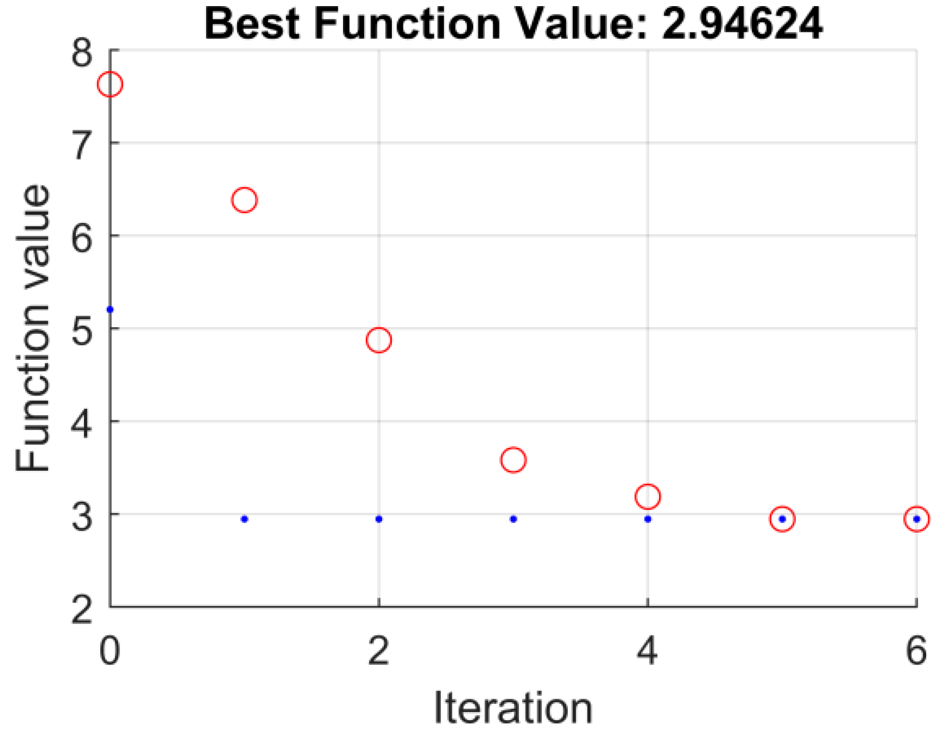
| Cost function y1 (14) | 5.0309 | 4.8601 | 2.9462 | 1.9462 |
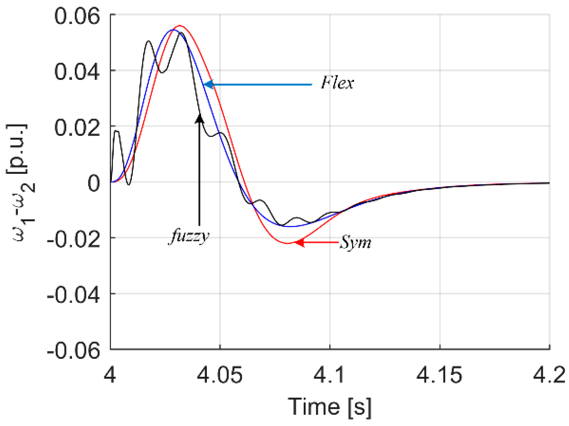
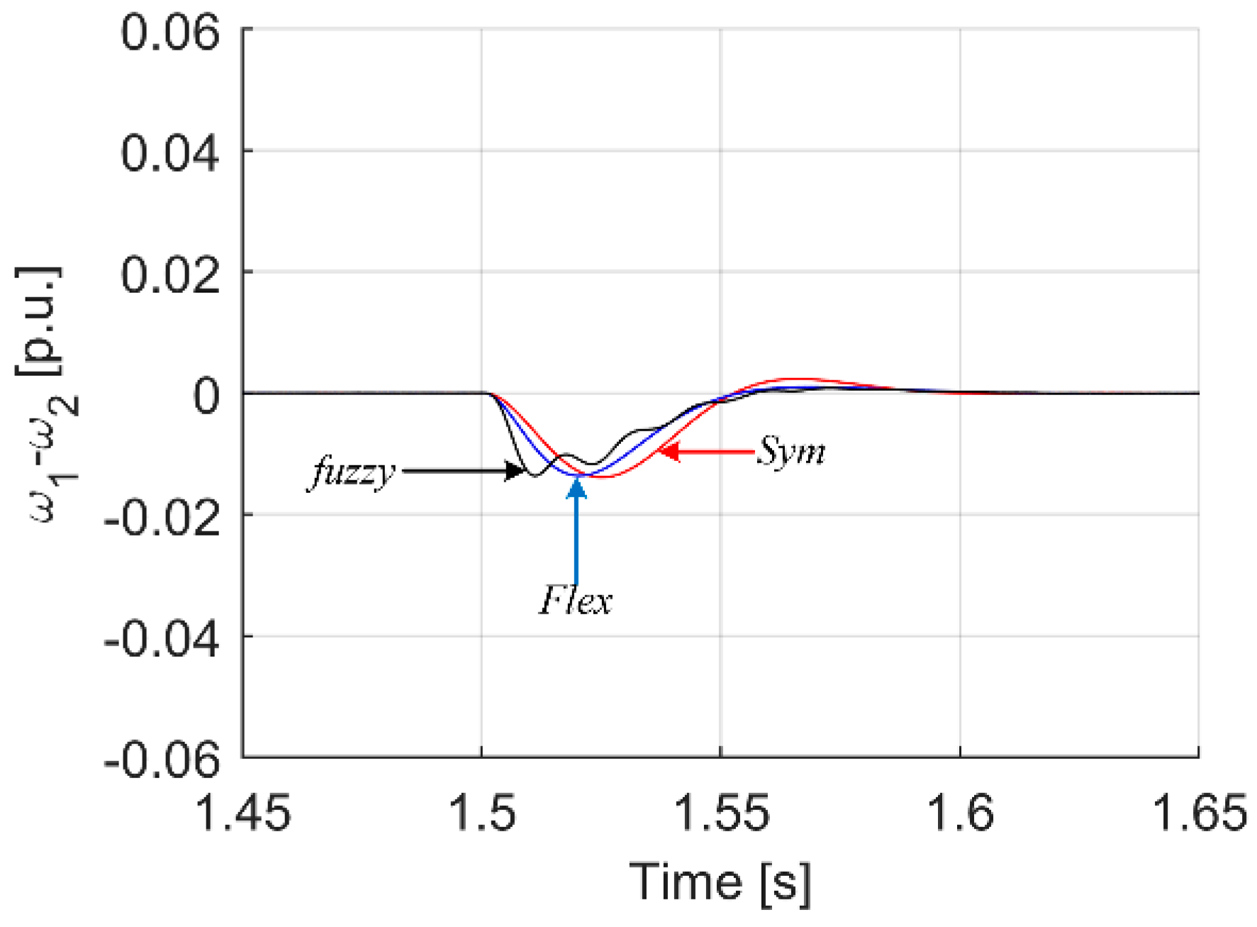
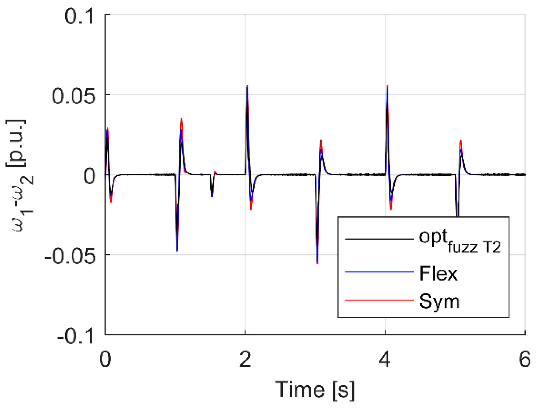
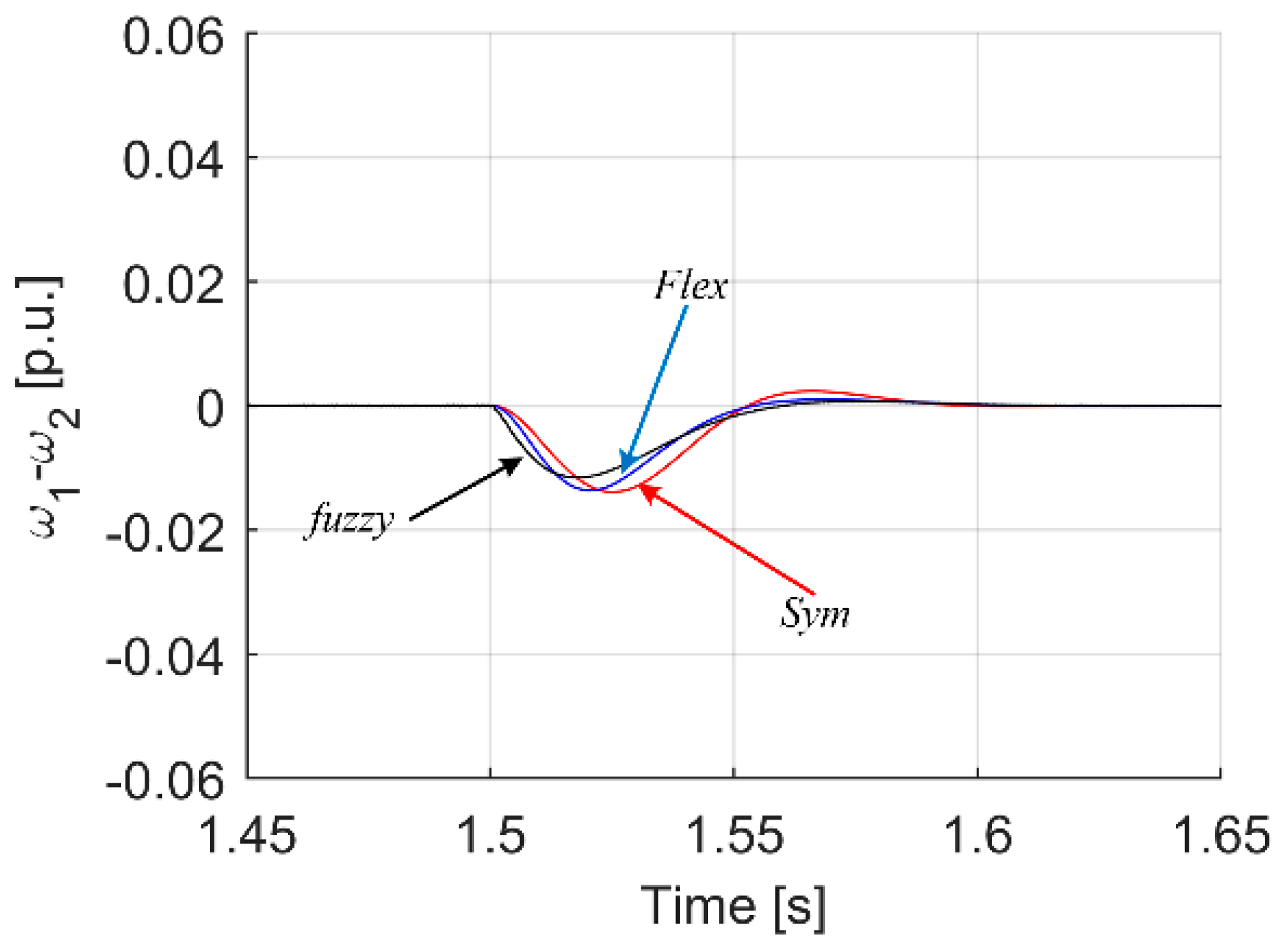
| Max(ω1 − ω2) dynamic state | 0.0560 | 0.0545 | 0.0548 | 0.0460 |
| Max(ω1 − ω2) load occurrence | 0.0139 | 0.0136 | 0.0137 | 0.0116 |
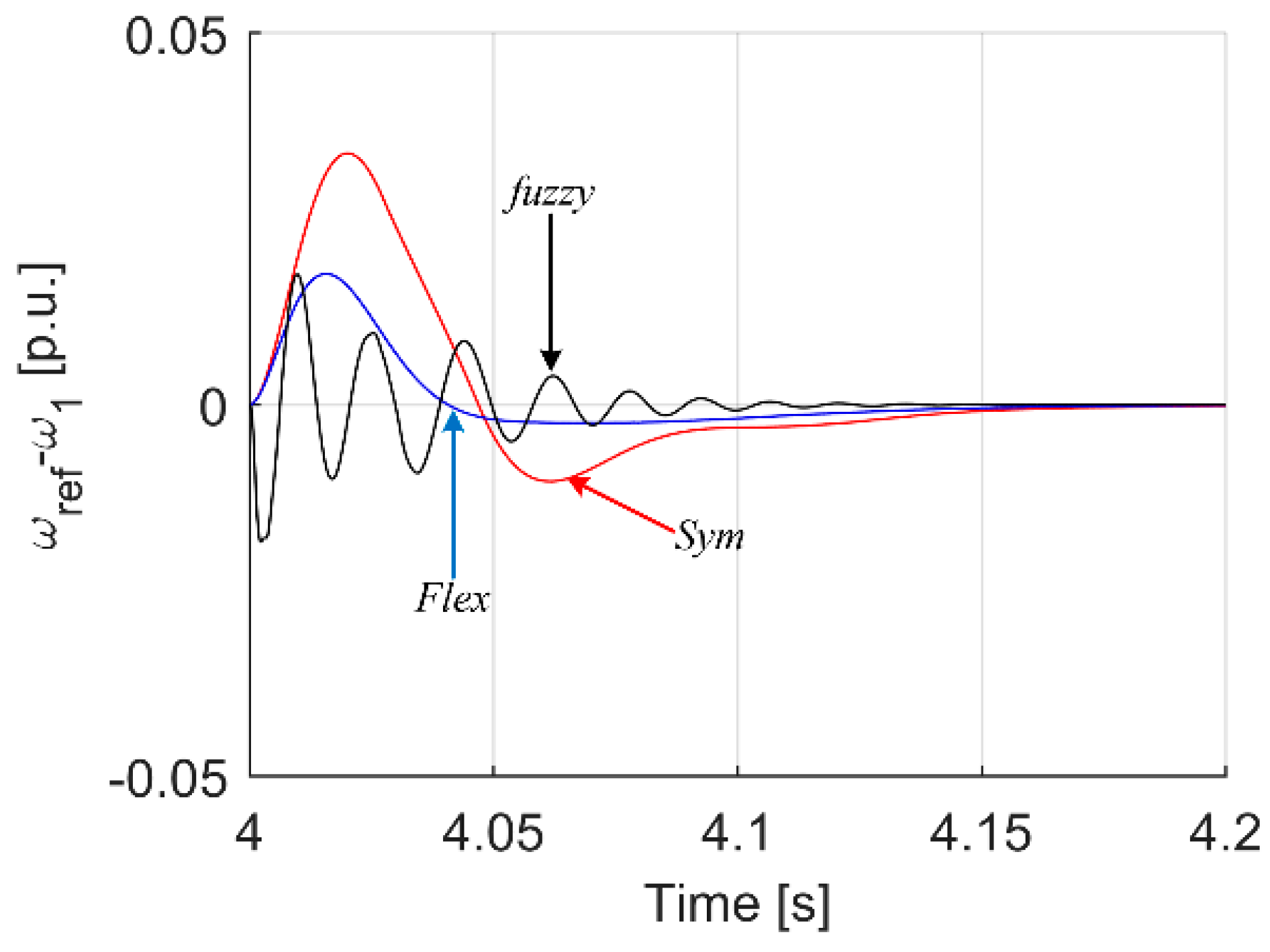
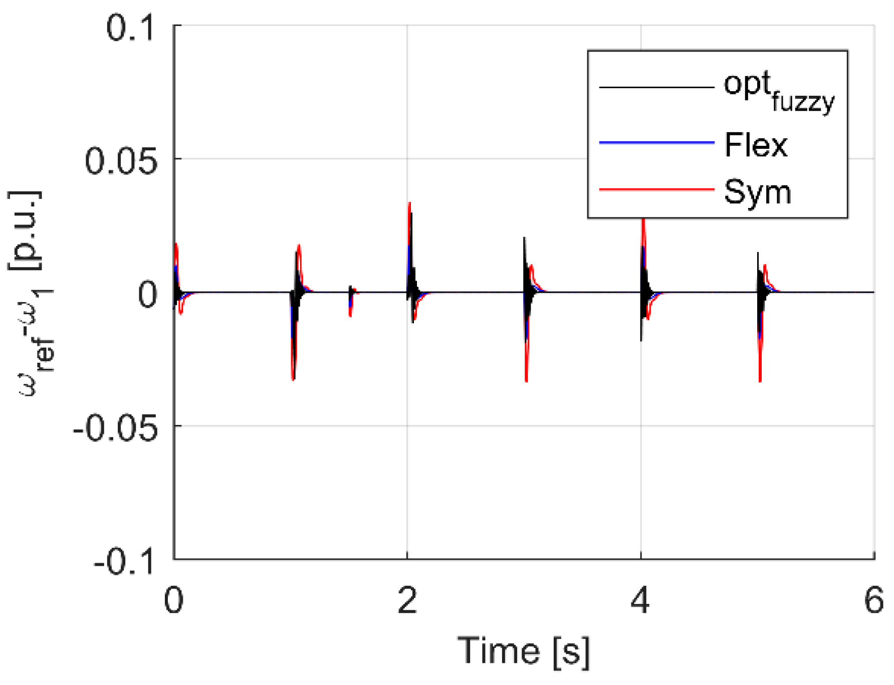
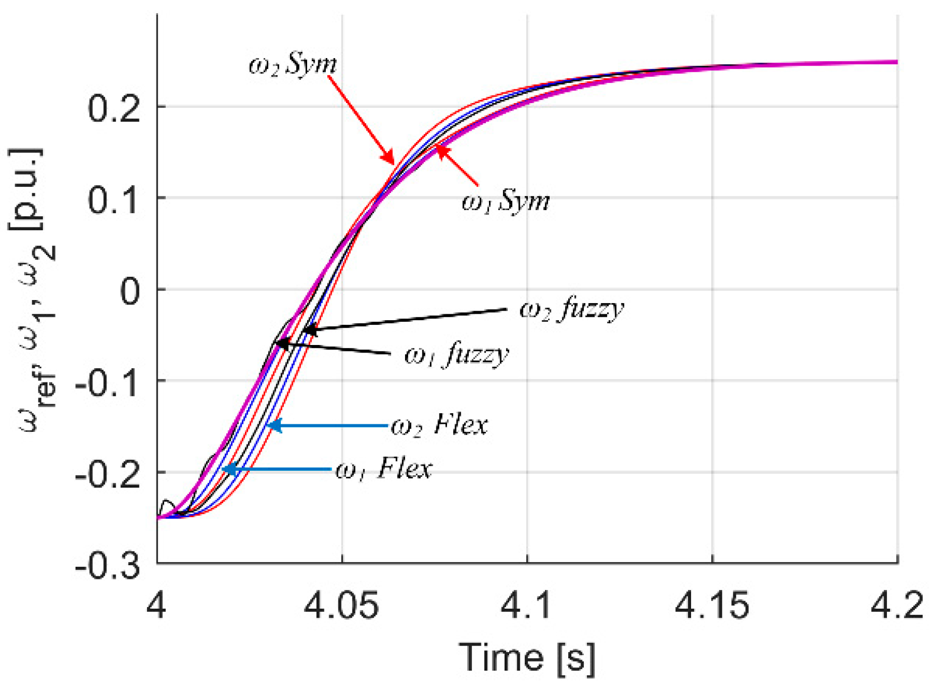
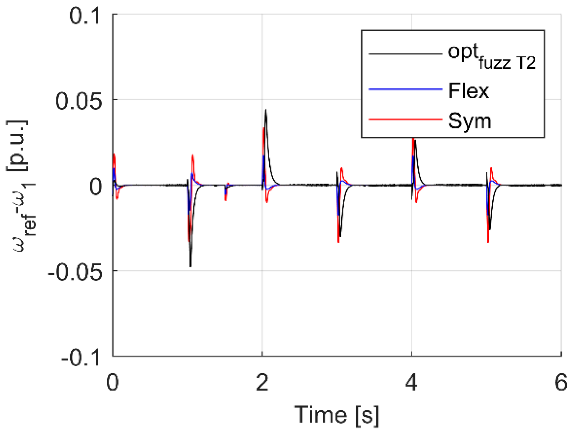
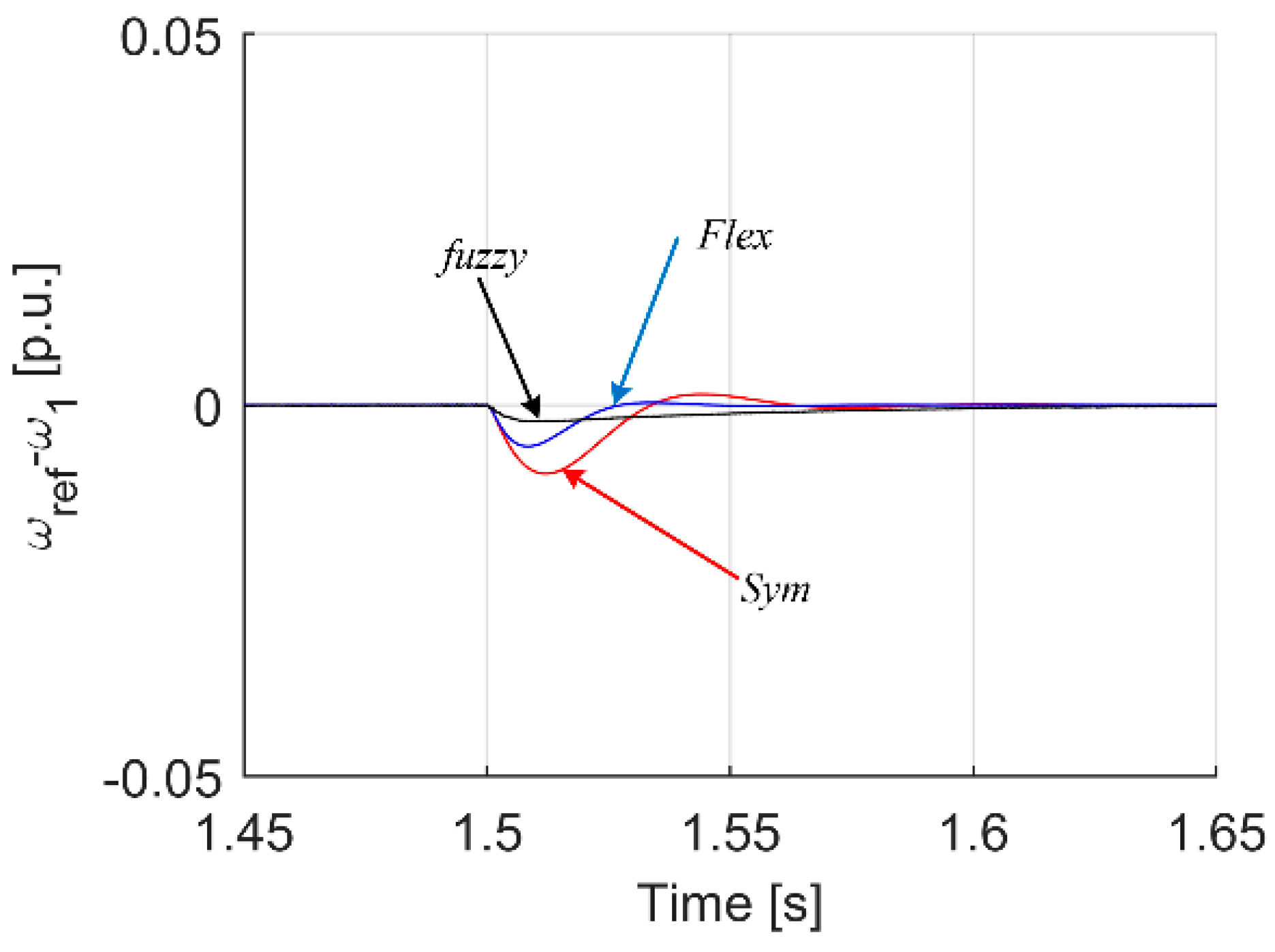
| Max(ωref − ω1) dynamic state | 0.0338 | 0.0176 | 0.0327 | 0.0480 |
| Max(ωref − ω1) load occurrence | 0.0093 | 0.0056 | 0.0033 | 0.0022 |
Publisher’s Note: MDPI stays neutral with regard to jurisdictional claims in published maps and institutional affiliations. |
© 2022 by the authors. Licensee MDPI, Basel, Switzerland. This article is an open access article distributed under the terms and conditions of the Creative Commons Attribution (CC BY) license (https://creativecommons.org/licenses/by/4.0/).
Share and Cite
Derugo, P.; Szabat, K.; Pajchrowski, T.; Zawirski, K. Fuzzy Adaptive Type II Controller for Two-Mass System. Energies 2022, 15, 419. https://doi.org/10.3390/en15020419
Derugo P, Szabat K, Pajchrowski T, Zawirski K. Fuzzy Adaptive Type II Controller for Two-Mass System. Energies. 2022; 15(2):419. https://doi.org/10.3390/en15020419
Chicago/Turabian StyleDerugo, Piotr, Krzysztof Szabat, Tomasz Pajchrowski, and Krzysztof Zawirski. 2022. "Fuzzy Adaptive Type II Controller for Two-Mass System" Energies 15, no. 2: 419. https://doi.org/10.3390/en15020419
APA StyleDerugo, P., Szabat, K., Pajchrowski, T., & Zawirski, K. (2022). Fuzzy Adaptive Type II Controller for Two-Mass System. Energies, 15(2), 419. https://doi.org/10.3390/en15020419