Updatable Probabilistic Evaluation of Failure Rates of Mechanical Components in Power Take-Off Systems of Tidal Stream Turbines

Abstract

This paper presents a method for the probabilistic evaluation of the failure rates of mechanical components in a typical power take-off (PTO) system of a horizontal-axis tidal stream turbine (HATT). The method is based on a modification of the method of the influence factors, when base failure rates, relevant influence factors and, subsequently, resulting failure rates are treated as random variables. The prior (i.e., initial) probabilistic distribution of the failure rates of a HATT component is generated using data for similar components from other industries, while taking into account actual characteristics of the component and site-specific operating and environmental conditions of the HATT. A posterior distribution of the failure rate is estimated numerically based on a Bayesian approach as new information about the component performance in an operating HATT becomes available. The posterior distribution is then employed to obtain the updated mean and lower and upper confidence limits of the failure rate. The proposed method is illustrated by applying it to the evaluation of the failure rates of two key components of the PTO system of a typical HATT—main seal and main bearing. In particular, it is shown that uncertainty associated with the method itself has a major influence on the failure rate evaluation. The proposed method is useful for the reliability assessment of both PTO designs of new HATTs and PTO systems of operating HATTs.

1. Introduction

Ocean and sea tides are an important source of renewable energy. Although the theoretical potential of tidal energy (1200 TWh/year) is much smaller than that of waves (29,500 TWh/year) or offshore wind (420,000 TWh/year), the former source of energy has one major advantage over the latter—since tides do not depend on weather their energy is well predictable both in the short and long term in contrast to that of waves and wind [1,2]. There are two main technologies for harvesting tidal energy—tidal barrages and tidal stream turbines. The former technology is much more mature and has a much larger installed capacity—521.5 MW for tidal barrages vs. 10.6 MW for tidal stream turbines in 2020 [2]. However, the tidal stream technology has a much larger potential since it has a lower capital cost, smaller environmental impact, and much wider choice of suitable sites compared to tidal barrages. The technology has been intensively developed in recent times and just reached a commercial stage; in particular, this concerns horizontal axis tidal turbines (HATTs), which are similar to typical wind turbines and, at present, the dominant type of tidal stream turbines [2,3].

There are currently plans to increase the installed capacity of tidal stream turbines up to 2.4 GW [2] which is a major step towards the commercialisation of the technology. However, this is still very far from attaining the technology’s full potential. To achieve the planned development and accelerate the penetration of tidal stream turbines into the energy market, large investments in this technology are required and for that a number of barriers need to be overcome. One of the barriers is uncertainty [4], a major source of which is the reliability of devices, including HATTs, used for tidal energy harvesting [5]. In addition, the reliability concerns were identified as the top-ranked non-commercial risk for both tidal stream turbines and wave energy converters, while poor reliability of these devices was mentioned as the main operational risk [6].

Why is the reliability of tidal stream turbines so important and what makes it such a large source of uncertainty? The answer to the first part of this question is that tidal stream turbines operate in harsh environments and, therefore, are likely to be subject to extreme loads and face an increased risk of failure. At the same time, their maintenance and repair are costly due to difficult and time-restricted accessibility. Thus, the energy production and costs depend strongly on the device reliability and, unsurprisingly, experts recommend introducing reliability modelling into the device design process [6]. The large uncertainty associated with the reliability is due to the fact that this is mainly untested technology so that historical data on failures of tidal stream turbines and their components are still extremely scarce. In this situation, the reliability of tidal stream turbines is often assessed using surrogate failure data from other industries (e.g., offshore oil and gas [7] or onshore wind), which may be roughly adjusted to specific operational conditions [8].

The approach employed in [8] was, in fact, a relatively simplistic implementation of a general technique, which has existed in system reliability for quite some time. The main idea of the technique is that generic failure data for a certain component are represented by its base failure rate, which is then adjusted to actual operating and environmental conditions of the component by multiplying it by the so-called “influence” factors (e.g., [9]). The technique is particularly useful for the reliability evaluation of design solutions at the early stages of their development and also very relevant for new technologies. Detailed implementation of the technique to various components of mechanical equipment (e.g., seals, bearings, valves, gears, etc.) was presented in [10]. The idea of applying this technique to marine energy converters was proposed in [11]. Since there are significant uncertainties associated with the influence factors and the technique itself, it was suggested, in the context of mechanical components of a HATT, to treat these factors and, subsequently, the resulting failure rate as random variables [12]. This probabilistic approach to failure rates was further developed and implemented for components of a pitch system of a HATT in [13]. In this work, the influence of specific characteristics of components of the pitch systems on their failure rates was taken into account. However, operating and environmental conditions of the HATT were treated as generic (i.e., not site-specific) and updating of the failure rates based on new data available after the turbine became operational was not considered. The reliability of mechanical components can also be assessed via a probabilistic analysis of their failure modes using advanced multi-physics models and taking into account uncertainties associated with the model parameters. Recent applications of this approach to blisks and blades of high-pressure turbines, including studies of relevant failure modes, can be found in [14,15,16,17,18].

The present paper describes a method for the probabilistic evaluation of the failure rates of mechanical components in a typical power take-off (PTO) system of a HATT. The method is based on the approach proposed in [12,19], i.e., the base failure rates, relevant influence factors and, subsequently, resulting failure rates are treated as random variables. In addition, the method addresses the issues mentioned above in connection to [13], i.e., (i) the influence factors account for the site-specific operating and environmental conditions of a HATT, and (ii) the probabilistic distributions of the failure rates can be updated using new data on the HATT’s performance collected during its operational life. The latter is based on a Bayesian approach that uses data for similar components from other industries to construct the prior distribution of the base failure rate for a component. To determine the parameters/distributions of the influence factors, in addition to the data from other industries, the approach accounts for actual characteristics of the component and site-specific operating and environmental conditions of the HATT. The prior distribution of the failure rate for the component is then generated by Monte Carlo simulation using the previously mentioned information about the base failure rate and influence factors. A posterior distribution of the failure rate can be estimated as new information about the component performance in the operating HATT becomes available. The posterior distribution can then be used to find the updated mean and lower and upper confidence limits of the failure rate. The proposed method is useful for the reliability assessment of both PTO designs of new HATTs and PTO systems of operating HATTs.

The rest of the paper is organised as follows. Section 2 presents the method. A brief description of a typical PTO system of a HATT and its reliability assessment are provided in Section 3. Section 4 covers a case study, which illustrates the application of the method to the evaluation of the failure rates of the main seal and main bearing in a typical HATT. This section starts with information about the HATT and its operating and environmental conditions, relevant for the failure rate evaluation of the seal and bearing. After that, the probabilistic evaluation of the failure rates of these two components, including their updating based on new data, is considered in detail. The paper ends with brief conclusions.

2. Probabilistic Estimation of Failure Rates

2.1. Bayesian Approach to Failure Rate Estimation

Estimating the failure rate of a mechanical (or electrical) component in a specific application becomes a challenging problem, when historical failure data for this component in this application are either unavailable or very scarce. This happens when the component either belongs to new technology (e.g., components of marine energy converters) or is highly reliable so that its failure is an extremely rare event (e.g., components in the nuclear industry). The lack of historical failure data creates significant uncertainty in relation to the failure rate estimation, which needs to be dealt with in a consistent and rational way. A Bayesian approach is a tool for doing this; e.g., it has been employed for the estimation of failure rates in the nuclear industry [20] and updating the failure rates of components of marine energy converters using test data [21].

In this approach, a prior (i.e., initial) distribution of the failure rate, π₀(λ), is defined based on initially available data (e.g., generic data from other industries) or/and expert opinions; in the case, when no data/knowledge is available a non-informative prior is used. New information obtained from observing the component performance over a certain period of time, e.g., the number of failures, n_f, over this period, is then utilised to update the distribution of the failure rate based on Bayes’ theorem [9]:

$$\pi \left(\lambda \right)=\frac{1}{c}L\left(n_f|\lambda \right){\pi }_0\left(\lambda \right)$$

(1)

where π(λ) is the posterior (i.e., updated) distribution of the failure rate, L(n_f|λ) the likelihood function (i.e., the likelihood of observing n_f failures given that the failure rate equals λ) and c the normalising factor, which is calculated as:

$$c=\underset{0}{\overset{\infty }{\int }}L\left(n_f|\lambda \right){\pi }_0\left(\lambda \right)d\lambda$$

(2)

The selection of the prior distribution π₀(λ) is considered next.

2.2. Choice of the Prior Distribution

The choice of the prior distribution depends on the amount and form of available data and on the way these data are treated. One of the forms of data, which is often used when the reliability of highly reliable systems is assessed, is expert opinions. In such case, a lack of historical failure data and infeasibility of obtaining necessary data from tests leave expert opinions as the only source of information. The ways of constructing prior distributions using this form of data were discussed in, e.g., [20,22].

For tidal stream turbines, the lack of failure data is primarily due to the fact that this is a new technology. Most of the components of tidal stream turbines are not unique and have been used in the past in other industries in various devices but under different operating and environmental conditions. Thus, generic data on failures of these components exist and, in principle, may be used to estimate their failure rates in this new application. However, in order to do that these generic failure data, which can be expressed in terms of a base (or generic) failure rate, need to be adjusted to specific conditions of the component in a tidal stream turbine. It should be noted that since the generic failure data are often obtained from different sources, significant uncertainty may be associated with the evaluation of the base failure rate.

A method for adjusting the failure rates of electronic components to different operating and environmental conditions was described in MIL-HDBK 217F [23]. According to this method, the failure rate, λ, of a component under specific operating and environmental conditions can be estimated by multiplying its base failure rate, λ_B (i.e., the failure rate for known standard operating and environmental conditions) by the so-called influence factors, C_j

$$\lambda ={\lambda }_B\prod _j{C}_j$$

(3)

The influence factors account for the effects of the differences, which exist between the specific and standard operating and environmental conditions (e.g., temperature, humidity, pressure, etc.) of the component, on its failures and, subsequently, on its failure rate. The method has also been applied to the estimation of the failure rates of mechanical components (e.g., [10,24]), in particular, those of the PTO system of a HATT [12,19].

The implementation of the method for mechanical components is usually more complicated than for electronic ones. A mechanical component often has a number of failure modes, which may be associated with its different parts. The number of factors affecting failures of a mechanical component may be rather large and these factors are usually specific for this particular component. Operating and environmental conditions affecting failures of mechanical components are much more variable compared to those of electronic components. At the same time, obtaining failure data from tests for mechanical components is often much more costly and time-consuming than for electronic equipment.

As a result, there is significant uncertainty associated with the estimation of the influence factors for mechanical components. Thus, it has been proposed to treat the base failure rate, the influence factors and, subsequently, the resulting failure rate as random variables [12]. The treatment of the failure rates as random variables is in line with existing databases on failures of various types of equipment, e.g., OREDA [7]; only the sources of uncertainty there and in the proposed approach are different. In the present paper, the method proposed in [12] is extended to account for new information, which can be obtained by observing the performance of operating tidal stream turbines. This means that the distribution of the failure rate, which is derived using generic failure data represented by the base failure rate and the influence factors, is treated as a prior distribution. Since the failure rate is expressed as the product of several random variables, i.e., the base failure rate and the influence factors—see Equation (3), according to the central limit theorem it can be assumed that it has a lognormal distribution:

$${\pi }_0\left(\lambda \right)=\frac{1}{\xi \lambda \sqrt{2\pi }}\exp \left[-\frac{1}{2{\xi }^2}{\ln }^2\left(\frac{\lambda }{m}\right)\right]$$

(4)

where m and ξ are the distribution parameters. These parameters can be found using Monte Carlo simulation, i.e., by generating values of λ using the distributions of λ_B and C_j’s and then fitting Equation (4) to the generated data. It is necessary to note that in order to account for uncertainties associated with the method itself, i.e., Equation (3), another multiplier, C_M, representing these uncertainties (usually called model uncertainty) will be added to the product in Equation (3) further in this study. C_M will be treated as a random variable with a mean of unity; its variability will represent our belief in the accuracy of the method and of the probabilistic models of λ_B and C_j’s used in the analysis.

2.3. Likelihood Function and Posterior Distribution

As in OREDA [7], it is assumed that for the purpose of the reliability calculation the failure rate λ of a component is independent of time. This assumption is commonly used in practice; moreover, due to the lack of historical failure data for a new technology such as tidal stream turbines, an estimation of the failure rate time-dependency is simply not feasible. However, the probabilistic distribution of λ can be updated over time as new information about the component’s performance becomes available. The updated (or posterior) distribution is obtained using Equation (1) and for that the likelihood function, which represents the new information, needs to be formulated. How this can be done is described in the following. Let us denote the number of failures of the component within the operating time interval t as N_f. Since for the reliability calculation, it is assumed that λ is time-independent then N_f, which is a random variable, follows the Poisson distribution with the parameter λt, i.e., the probability of exactly n_f failures within the time interval t is given by the following formula:

$$P\left[N_f\left(t\right)=n_f\right]=\frac{{\left(\lambda t\right)}^{n_f}}{n_f!}\exp \left(-\lambda t\right)$$

(5)

Equation (5) also gives the likelihood of observing exactly n_f failures of the component over operating time t when the failure rate is λ:

$$L\left(n_f|\lambda \right)=\frac{{\left(\lambda t\right)}^{n_f}}{n_f!}\exp \left(-\lambda t\right)$$

(6)

Substituting Equation (6) into Equation (1) leads to the following formula for the posterior distribution of the failure rate:

$$\pi \left(\lambda \right)=\frac{1}{c}\exp \left[-\frac{1}{2{\xi }^2}{\ln }^2\left(\frac{\lambda }{m}\right)\right]\frac{{\left(\lambda t\right)}^{n_f}}{n_f!}\exp \left(-\lambda t\right)$$

(7)

where the normalising factor is:

$$c=\underset{0}{\overset{\infty }{\int }}\exp \left[-\frac{1}{2{\xi }^2}{\ln }^2\left(\frac{\lambda }{m}\right)\right]\frac{{\left(\lambda t\right)}^{n_f}}{n_f!}\exp \left(-\lambda t\right)d\lambda$$

(8)

The latter can be calculated numerically. It is worth to note that Equation (7) represents the probability density function of the failure rate; hence, after π (λ) has been obtained, statistical characteristics of the failure rate (e.g., mean, variance, lower and upper confidence limits) can easily be calculated numerically in accordance with their definitions.

It should also be noted that since the failure rate is assumed to be time-independent it is unimportant whether the information about the component’s performance comes from a single device or a group of identical devices. For example, whether one device has operated without failure of the component for t years or t identical devices have operated in similar conditions without such failure for one year; in both cases, the time interval in the above equations will be equal to t and n_f = 0.

3. Power Take-Off (PTO) System of a Horizontal Axis Tidal Turbine (HATT) and Its Reliability Assessment

The PTO system of a HATT may be either direct drive, when a rotor is connected directly to a generator, or indirect drive, when a rotor is connected to a generator via a gearbox. The rotational speed of the turbine rotor may be either fixed or variable. Turbine blades may be either fixed pitch or have variable (controlled) pitch. There are a number of other characteristics that may be used to distinguish different configurations of the PTO system of a HATT.

The PTO system, the components of which will be considered further in the paper in the context of the probabilistic evaluation of the failure rates, is an indirect drive with a fixed-speed rotor, a mechanical gearbox and pitch-controlled blades. It also includes brakes, couplings, generator and controllers. The blades are connected through a pitch control system to a hub, which is attached to a low-speed shaft. The latter transmits power from the rotor to the generator via the gearbox. A mechanical type seal (main seal) is installed on the shaft to prevent the entry of seawater into the gearbox and retain lubricating oil inside it. A locating (main) bearing of the low-speed shaft is positioned immediately after the main seal.

It is assumed that the PTO system is functioning when all its components/subsystems are functioning. It is also assumed that failures of different components/subsystems are independent events. Based on these assumptions the PTO system can be modelled as a series system and its reliability block diagram is shown in Figure 1.

Since the PTO system is modelled as a series system its reliability over time t, R_PTO(t), can be estimated as (e.g., [9]):

$$R_{PTO}\left(t\right)=\prod _i{R}_i\left(t\right)$$

(9)

where R_i(t) is the reliability of the i-th component/subsystem. The latter is calculated as [9]:

$$R_i\left(t\right)=\exp \left(-{\lambda }_{i}t\right)$$

(10)

where λ_i is the failure rate of the component, because it is assumed in this study that the failure rate is treated as time-independent for the purpose of the reliability calculation. A case study illustrating the application of the method described in the previous section to the evaluation of the failure rates of key mechanical components of the PTO system such as the main seal and main bearing is presented next. These two components are critical for the operation of a HATT—if they fail, then the entire PTO system fails (see the reliability block diagram in Figure 1). Moreover, their failure can lead to failures of other PTO components, while their replacement in the case of failure is time-consuming and expensive (especially this concerns the main bearing).

4. Case Study: Evaluation of the Failure Rates of PTO Components of HATT

4.1. Characteristics of HATT’s Site

Characterisation of a site intended for the deployment of tidal stream turbines requires the measurement of water level and current velocity profile over a significant period of time [25]. However, this case study is solely to illustrate the previously described method and for this purpose very limited data, namely variations of the speed of bi-directional tidal current at the level of the turbine rotor hub over 24 h (see Figure 2), are sufficient. The data are used in the following to estimate the proportion of the time when the HATT is working as well as variations of the turbine power and thrust with time; of course, much longer (at least 30-day) records of tidal current velocity should be employed in practical applications.

As can be seen from Figure 2, there is a significant difference between flood and ebb tide. Peak flood current speeds are faster (up to 3 m/s) and occur over longer periods of time than peak ebb speeds (which do not exceed 2.4 m/s). A site with such current characteristics may not be a good choice for deploying tidal stream turbines. However, this is not important herein since, as noted above, the example is for illustrative purposes only.

4.2. Main Parameters of HATT

An indirect drive HATT with the following parameters is considered: rated current speed 2.4 m/s; the corresponding mechanical power on the shaft 600 kW; two-bladed 16 m-diameter rotor; rotational speed of the rotor 14 rpm; the blades are pitch controlled. The average water depth at the rotor hub level under operating conditions is 15 m. When in operation the blades are filled with sea water [26]. The NREL S814 section [27] is adopted for the blade section. Forces acting on the blades are calculated using the NWTC Engineering Tool AeroDyn [28], which is based on the blade element momentum theory. The drag and lift coefficients needed for the analysis have been obtained using the two-dimensional vortex panel code XFoil [29]. The calculated power versus current-speed curve and the corresponding trust are shown in Figure 3. It is assumed that the blade pitch angle is adjusted to achieve the maximum power at current speeds below the rated speed and to limit the power to the rated value at current speeds above the rated speed. The cut-in speed is set at 1 m/s.

Variations of the turbine power and thrust with time are obtained using the data from Figure 2 and Figure 3 and shown in Figure 4. The results are presented as 10 min averages. This allows to clearly see major changes in the power and trust with time, sufficient for further analysis, and also in line with existing guidelines [25]. Actual variations of the power and trust with time depend on fluctuations in the tidal current speed and on the performance of the controller.

According to the results shown in Figure 4, the HATT operates 65% of the time. It is also important to note that when the HATT does not operate, the thrust is obviously not necessarily equal to zero. However, in this case study values of the thrust are only needed to estimate the dynamic equivalent load on the main bearing (i.e., load when the bearing is operating); thus, values of the thrust in static condition are not important for the following analysis and not shown.

The low-speed shaft of the PTO system transfers loads from the rotor to the gearbox as shown in Figure 5. The torque acting on the shaft at the rated current speed, M_r, is 410 kNm (see Figure 3). Other loads acting on the shaft include the axial thrust N_a, the weight of the rotor G_r (which is estimated to be 20 kN in the submerged condition), and the weight of the shaft G_s. The shaft dimensions are: l₁ = 0.6 m, l₂ = 0.45 m and l₃ = 0.5l₁. The shaft is hollow to accommodate power cables of a pitch actuation system. The shaft is made of normalised AISI 4140 steel with the yield strength of 655 MPa. Based on the applied loads and dimensions the required external diameter of the shaft is estimated to be 220 mm (internal 100 mm) [30] so that G_s = 1.4 kN.

4.3. Evaluation of the Failure Rate of the Main Seal

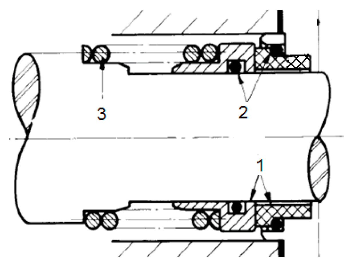
A rotating shaft seal is installed on the low-speed shaft to prevent leakage of seawater into the turbine nacelle (or the gearbox if the drive train is not enclosed in a nacelle). It is assumed that a mechanical face seal is used for this purpose. The main groups of parts of this type of seal are shown in Figure 6. In accordance with the dimensions of the low-speed shaft, the balance (or sliding) diameter of the seal is 220 mm. The inside and outside diameters of the sealing surface are 221.6 mm and 229.6 mm, respectively. The seal face material combination is carbon/silicon carbide, which demonstrated excellent performance in seawater applications (e.g., [31]).

In principle, the operating life of a mechanical face seal should be controlled by wear out of the seal face. However, a relatively small proportion of mechanical seals fail due to wear [32]. Apart from excessive wear, other common modes of seal failure are separation of faces, fatigue-like surface embrittlement, thermal-stress cracking, abrasive removal of surface material and corrosion. The reliable performance of a mechanical face seal mainly depends on the conditions at the seal interface, particularly on the lubrication regime between the seal faces. Most mechanical seals operate under a mixed lubrication regime when the load between the seal faces is carried partly by fluid pressure and partly by mechanical contact (e.g., [33]). Thus, the parameters which affect the operating life and failures of mechanical seals include pressure, sliding velocity and temperature at the seal interface, surface finish of seal faces, properties of the surrounding fluid and its contamination.

Thus, the failure rate of a mechanical face seal, λ_S, Equation (3) can be calculated as [10]:

$${\lambda }_S={\lambda }_{S,B}{C}_Q{C}_F{C}_{\nu }{C}_T{C}_N{C}_{PV}{C}_M$$

(11)

where λ_S,B is the base failure rate, C_Q the influence factor for allowable leakage, C_F the influence factor for surface finish, C_ν the influence factor for fluid viscosity, C_T the influence factor for seal face temperature, C_N the influence factor for contamination, C_PV the influence factor for the pressure-velocity (PV) parameter, and C_M takes into account the model uncertainty.

The base failure rate is estimated using results of 274 tests presented in [32]. Seals in the tests were made of carbon graphite and tungsten carbide and operated in water; the water temperature was not reported. Statistical analysis of the test results yielded the mean of 46.9 failures per million hours (pmh) and standard deviation of 23.3 pmh. The average PV parameter in the tests was 6.9 MPa∙m/s. In absence of more detailed information, it is assumed that the variability of the base failure rate can be described by a lognormal distribution.

According to [10], C_Q = 4.2 − Q_f, where Q_f is the allowable leakage rate under conditions of usage. Since the leakage should not be allowed Q_f ≈ 0 so that C_Q = 4.2. For the material combination carbon/silicon carbide typical surface finish in RMS is 0.125 μm [32]. Thus, according to [10], C_F = 1. The tests results used to estimate λ_S,B were obtained for seals operating in water, while the seal in the HATT operates in seawater. The influence factor for viscosity is C_ν = ν_w/ν_sw [10], where ν_w and ν_sw are the dynamic viscosities of water and seawater, respectively. The viscosity of seawater is slightly higher than that of water, e.g., for T = 10 °C ν_w = 1.27 × 10⁻³ Pa∙s and ν_sw = 1.38 × 10⁻³ Pa∙s. Since C_v should be slightly less than unity in the following analysis it is conservatively assumed that C_ν = 1.

As noted above, no information about the temperature was provided for the test results. Since values of the pressure and sliding velocity at the seal interface were much higher in the tests than in the seal under consideration, it is expected that the temperatures in the tests were also higher. This means that C_T should be less than unity [10]; because of the lack of more concrete data, it is conservatively assumed that C_T = 1.

Seawater around the seal may contain abrasive solid particles like sand; therefore, the seal environment is characterised as rather harsh. Due to a lack of reliable data on actual contamination of the seal environment, C_N is treated as a random variable, which can take values between 1 and its upper bound 4 for a harsh environment [10]. It is assumed that C_N is modelled as a beta random variable defined on (1, 4) with mean 3.5 and coefficient of variation (COV) 0.10.

The influence factor for the PV parameter is determined as C_PV = PV_OP/P_VB [10], where PV_OP and PV_B are the PV parameters for actual seal operation and for the base case operation, respectively. According to the information on the tests, which results were employed to determine λ_S,B, P_VB = 6.9 MPa∙m/s. PV_OP can be estimated based on the net face pressure as [32]:

$$P{V}_{OP}=\left[\mathsf{\Delta }p\left(B-K\right)+p_s\right]V$$

(12)

where Δp is the pressure differential across the seal, B the balance ratio (=1.2 [33]), K the pressure gradient factor (=0.5), p_s the pressure at the seal interface due to the spring (= 0.2 MPa), and V the sliding velocity at the seal face (= 0.33 m/s for the rotor rotational speed of 14 rpm). The pressure inside the nacelle is assumed to be atmospheric. Hence, since the average water depth at the rotor hub level is 15 m, the mean Δp is around 0.15 MPa. However, Δp fluctuates due to the water level variations caused by tides and waves and effects of water flow. It is estimated that these fluctuations can result in changes of Δp within ±0.035 MPa. Thus, Δp is presented as the sum of its mean value (= 0.15 MPa) and a beta random variable δp defined on (−0.035, 0.035) with zero mean and standard deviation 0.0105, i.e., Δp = 0.15 + δp (MPa).

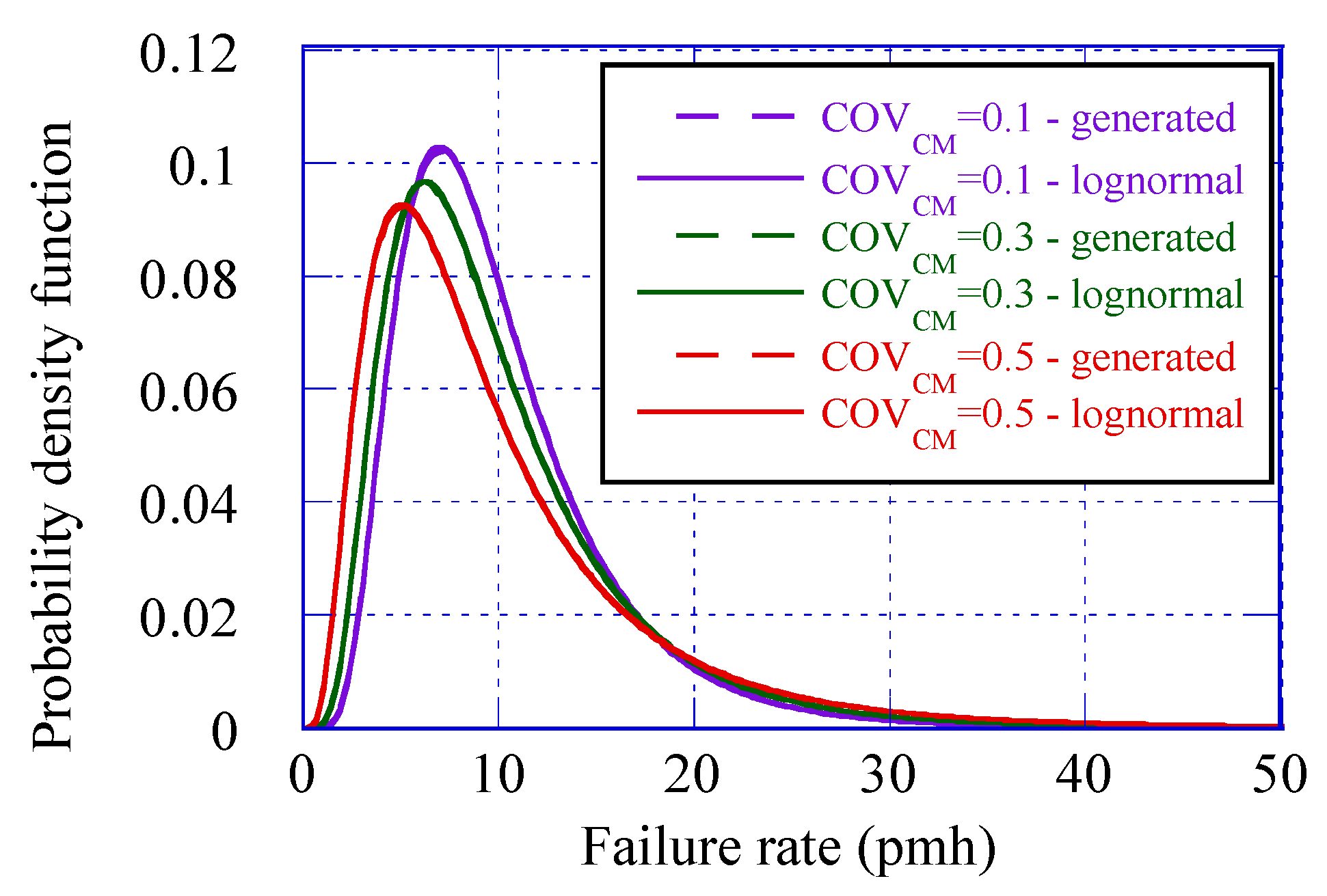
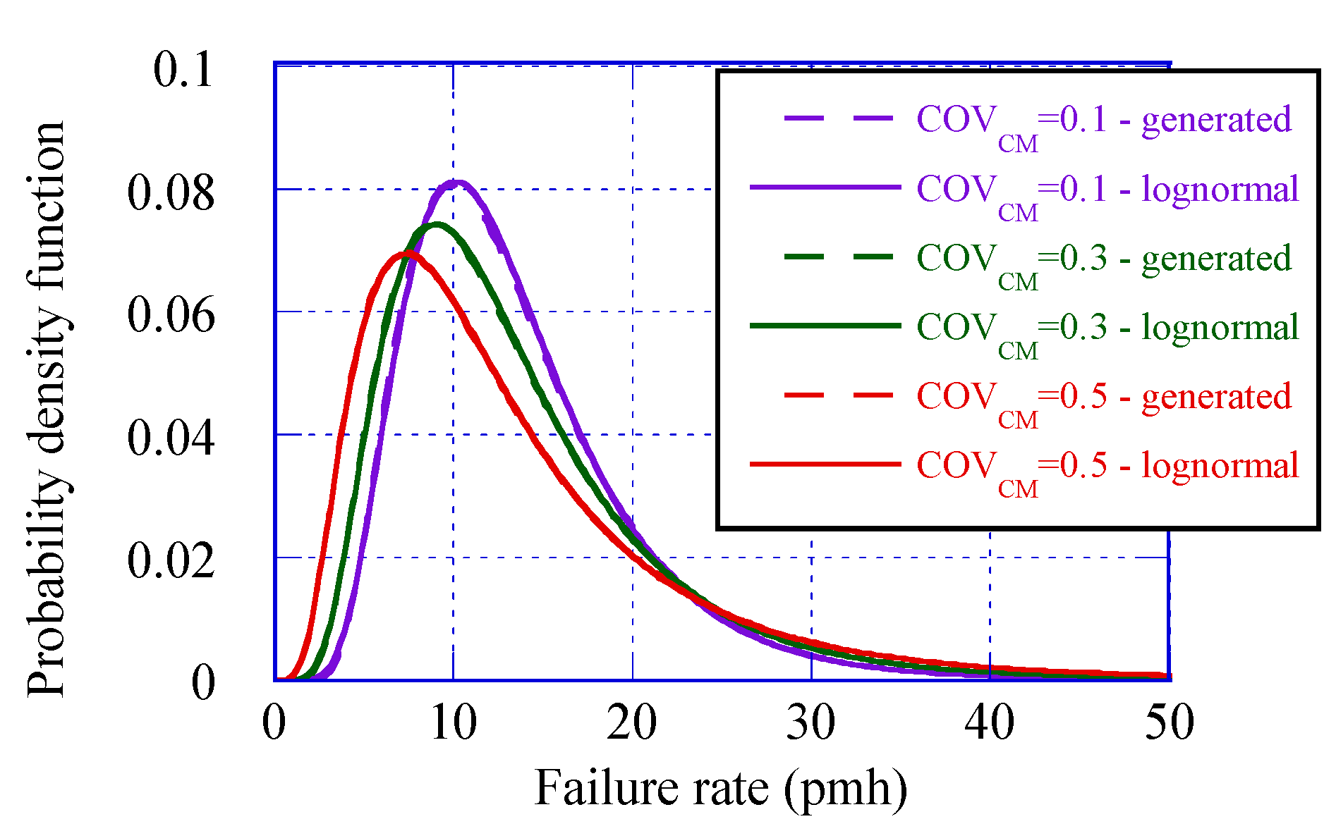
As explained previously, C_M represents the model uncertainty or, in other words, various uncertainties associated with the method of the influence factors, i.e., Equation (11) for the seal. The latter equation is used to construct a prior distribution of the failure rate so that C_M can also be used to represent the degree of belief in this prior. In the following, C_M will be treated as a lognormal random variable with a mean of unity. Three values of its COV, denoted further as COV_CM, representing different degrees of belief will be considered: 0.1—strong belief, 0.3—medium belief, and 0.5—weak belief. Since a lognormal distribution is skewed to the right its choice for C_M also means that results obtained by the proposed method will tend to overestimate the failure rate, i.e., to be on a conservative side.

Initially, as explained previously, a prior distribution of the failure rate of the seal is obtained by generating values of the random variables described above and substituting them into Equation (11). This is done using Monte Carlo simulation. The generated prior distribution of the failure rate is then approximated by a lognormal distribution; since the failure rate is the product of several random variables (see Equation (11)) it is expected, in accordance with the central limit theorem (e.g., [9]), that its distribution approaches a lognormal distribution. Figure 7 shows the generated prior distributions of λ_S and their lognormal approximations (more exactly, probability density functions of the distributions) for the three different values of COV_CM. As can be seen, there is an excellent agreement between the generated distributions and their lognormal approximations (at the scale of the figure, no difference between the generated distributions and their approximations can even be observed). In addition to Figure 7, the prior estimates of the failure rate of the seal obtained are presented in

Table 1. Characteristics of prior and posterior (after one calendar year of operation) distributions of the failure rate of the seal.

COVCM	nf (Failures)	μλs (pmh)	COVλs	λS,0.05 (pmh)	λS,0.95 (pmh)
0.1	prior distribution
	−	10.1	0.52	3.9	19.9
	posterior distribution
	0	9.9	0.52	4.0	19.6
	1	12.6	0.52	5.0	24.8
	2	15.9	0.51	6.4	31.4
	3	20.1	0.51	8.1	39.7
0.3	prior distribution
	−	10.1	0.61	3.3	21.6
	posterior distribution
	0	9.9	0.60	3.4	21.1
	1	13.4	0.60	4.6	28.7
	2	18.3	0.60	6.3	39.0
	3	24.8	0.59	8.6	52.6
0.5	prior distribution
	−	10.1	0.76	2.5	24.2
	posterior distribution
	0	9.7	0.74	2.6	23.3
	1	15.1	0.73	4.1	35.9
	2	23.2	0.72	6.3	54.7
	3	35.2	0.70	9.8	82.1

in the format employed in the OREDA database [7], i.e., in terms of its mean value, μ_λ,s, COV_λ,s (instead of standard deviation given in [7]) and 90% uncertainty interval defined by its lower (5%) and upper (95%) limits (denoted as λ_S,0.05 and λ_S,0.95, respectively).

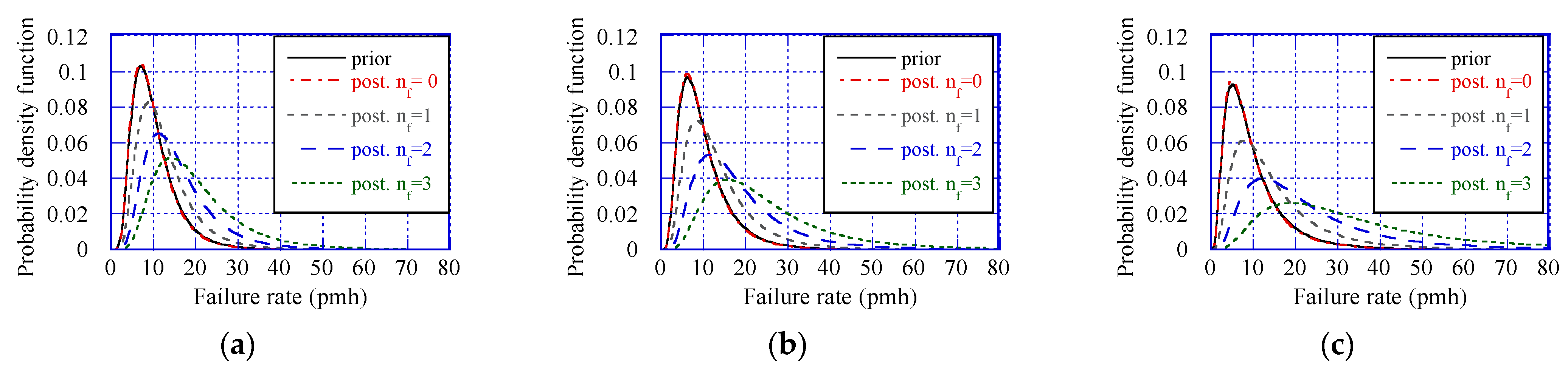
To illustrate the updating, i.e., how new information about the seal performance in operating HATT(s) may affect the distribution and the main characteristics λ_S, several possible scenarios have been considered. First, four possible outcomes—no failure and one, two and three failures, for a single main seal in an HATT, which has been in operation for one calendar year, have been taken into account. Results of this analysis for the three values of COV_CM are presented in Figure 8 and Table 1 in terms of the posterior distributions and the main characteristics of λ_S, respectively. As can be seen, the information that one seal has operated during one calendar year without failure has a very small effect on the distribution of λ_S (the posterior distributions for n_f = 0 are practically identical to the corresponding priors) and, subsequently, on its main characteristics. This occurs because the probability of the seal failure within one calendar year based on its prior mean value is relatively low (less than 0.06) so that this outcome is more or less expected. The effect of this new information is slightly more noticeable but still small when belief in the prior distribution is weak (i.e., COV_CM = 0.5)—the mean value of λ_S and the width of the uncertainty interval marginally decrease. However, if the seal fails during one calendar year of its operation this significantly affects the distribution and the main characteristics of λ_S—the distribution becomes flatter, its mean value and standard deviation increase, and subsequently the uncertainty interval widens. It is interesting to note that the COVs of the posterior distributions change very little compared to their values of the corresponding priors (even slightly decrease) but the increase in the mean values results in a major increase in values of the standard deviations. Obviously, as the number of failures increases, their influence on the distribution of λ_S becomes more prominent.

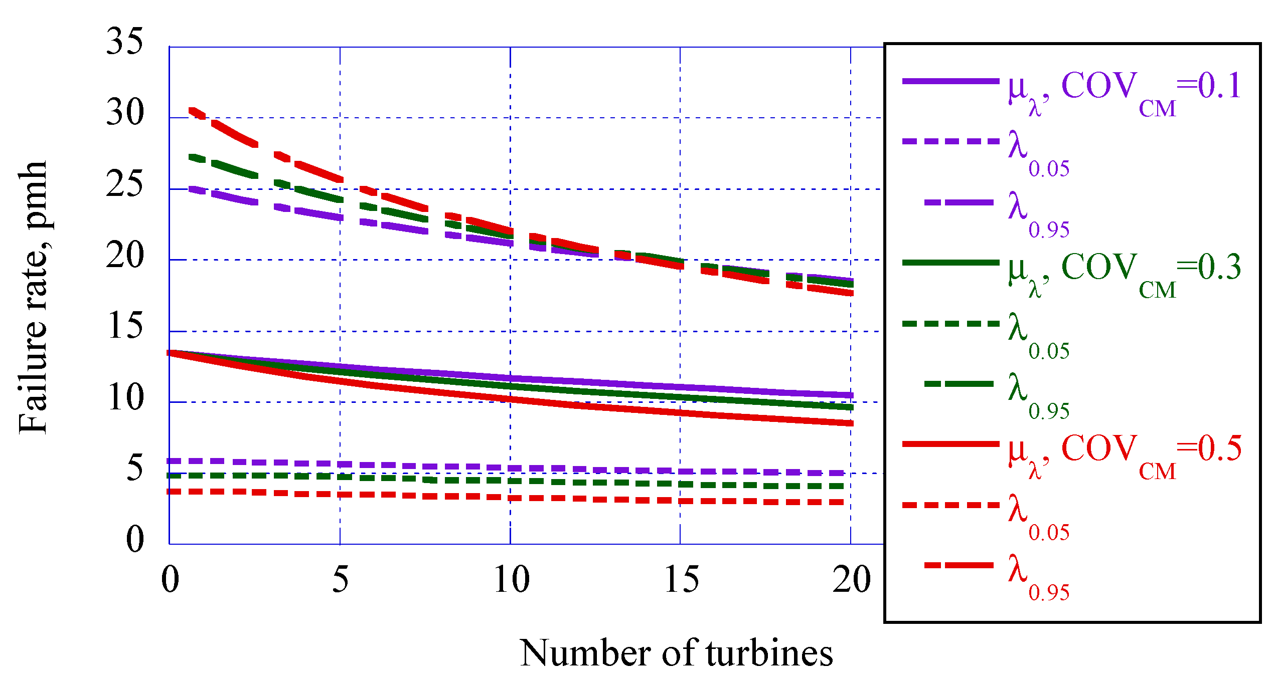
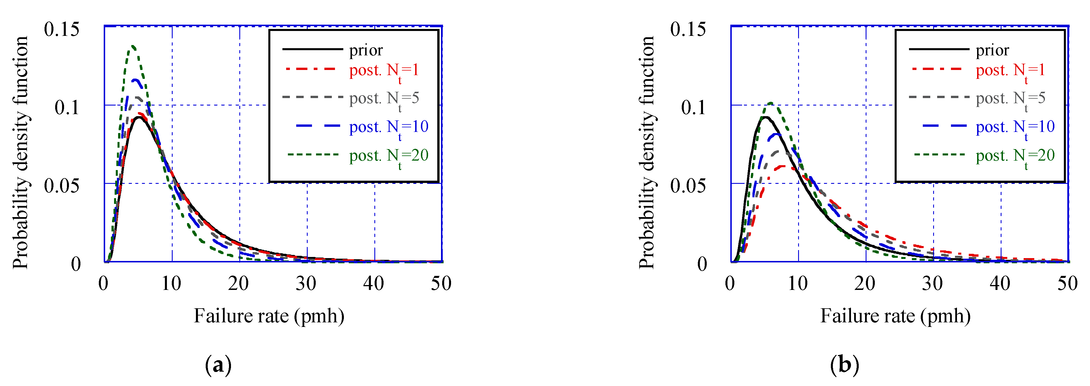
Second, the influence on new information is examined when an array of the identical HATTs (described previously) has been in operation for one calendar year. Three values of the number of the HATTs in the array, N_t, are considered—5, 10 and 20. Two possible outcomes are considered—no failures of the seal and one failure across all HATTs in the array. The main characteristics of the seal’s failure rate after updating are presented in

Table 2. Characteristics of posterior distributions of the failure rate of the seal for an array of identical HATTs after one calendar year of operation.

COVCM	Nt	nf = 0				nf = 1
		μλs (pmh)	COVλs	λS,0.05 (pmh)	λS,0.95 (pmh)	μλs (pmh)	COVλs	λS,0.05 (pmh)	λS,0.95 (pmh)
0.1	1	9.9	0.52	4.0	19.6	12.6	0.52	5.0	24.8
	5	9.4	0.50	3.8	18.3	11.7	0.50	4.8	22.7
	10	8.8	0.48	3.7	16.9	10.8	0.48	4.6	20.7
	20	7.9	0.46	3.4	14.8	9.6	0.45	4.2	17.7
0.3	1	9.9	0.60	3.4	21.1	13.4	0.60	4.6	28.7
	5	9.1	0.58	3.2	19.2	12.2	0.57	4.3	25.3
	10	8.4	0.55	3.1	17.3	11.0	0.54	4.1	22.3
	20	7.4	0.52	2.9	14.7	9.4	0.50	3.7	18.4
0.5	1	9.7	0.74	2.6	23.3	15.1	0.73	4.1	35.9
	5	8.8	0.69	2.5	20.3	12.9	0.67	3.7	29.5
	10	7.9	0.65	2.3	17.7	11.2	0.62	3.5	24.7
	20	6.7	0.61	2.1	14.5	9.1	0.57	3.1	19.3

for the three values of COV_CM; the results for one HATT have been included in the table for ease of comparison. In addition, the posterior distributions of λ_S for COV_CM = 0.5 are presented in Figure 9 for visual comparison. As expected, as the number of the identical seals for which the new information becomes available increases, the impact of this information on the evaluation of the seal’s failure rate becomes more significant. In the case of no observed failure (i.e., n_f = 0), both the mean value and COV of the failure rate steadily decrease as the number of seals increases. If one failure has occurred, then for the smaller numbers of the seals (i.e., 1, 5 and 10) the mean value of λ_S and uncertainty associated with its evaluation increase compared to the prior data. However, when N_t = 20, the mean value and the uncertainty become smaller than the corresponding priors. As expected, the impact of the new information is stronger when belief in the prior distribution of λ_S is weaker (i.e., the strongest for COV_CM = 0.5).

4.4. Evaluation of the Failure Rate of the Main Bearing

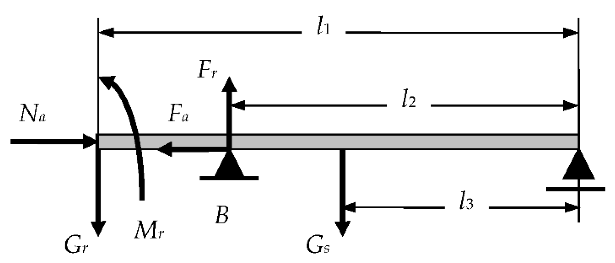
The main bearing is located at point B (see Figure 5). Magnitudes of the horizontal and vertical support reactions acting at B on the shaft are equal to the bearing axial, F_a, and radial, F_r, loads, respectively. The equilibrium of the shaft requires F_a = N_a and F_r = (l₁/l₂)(G_r + 0.5G_s). 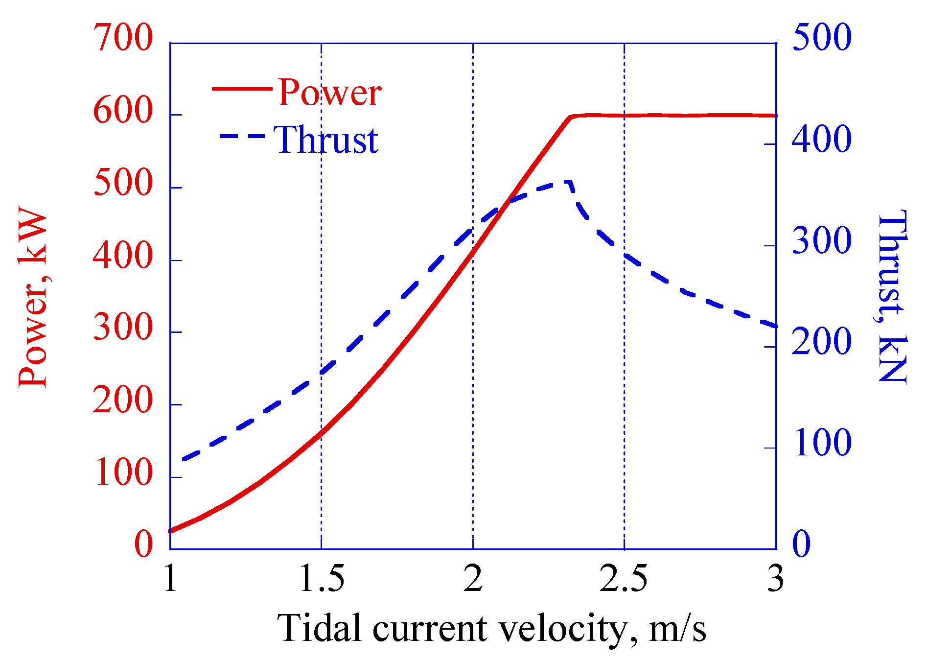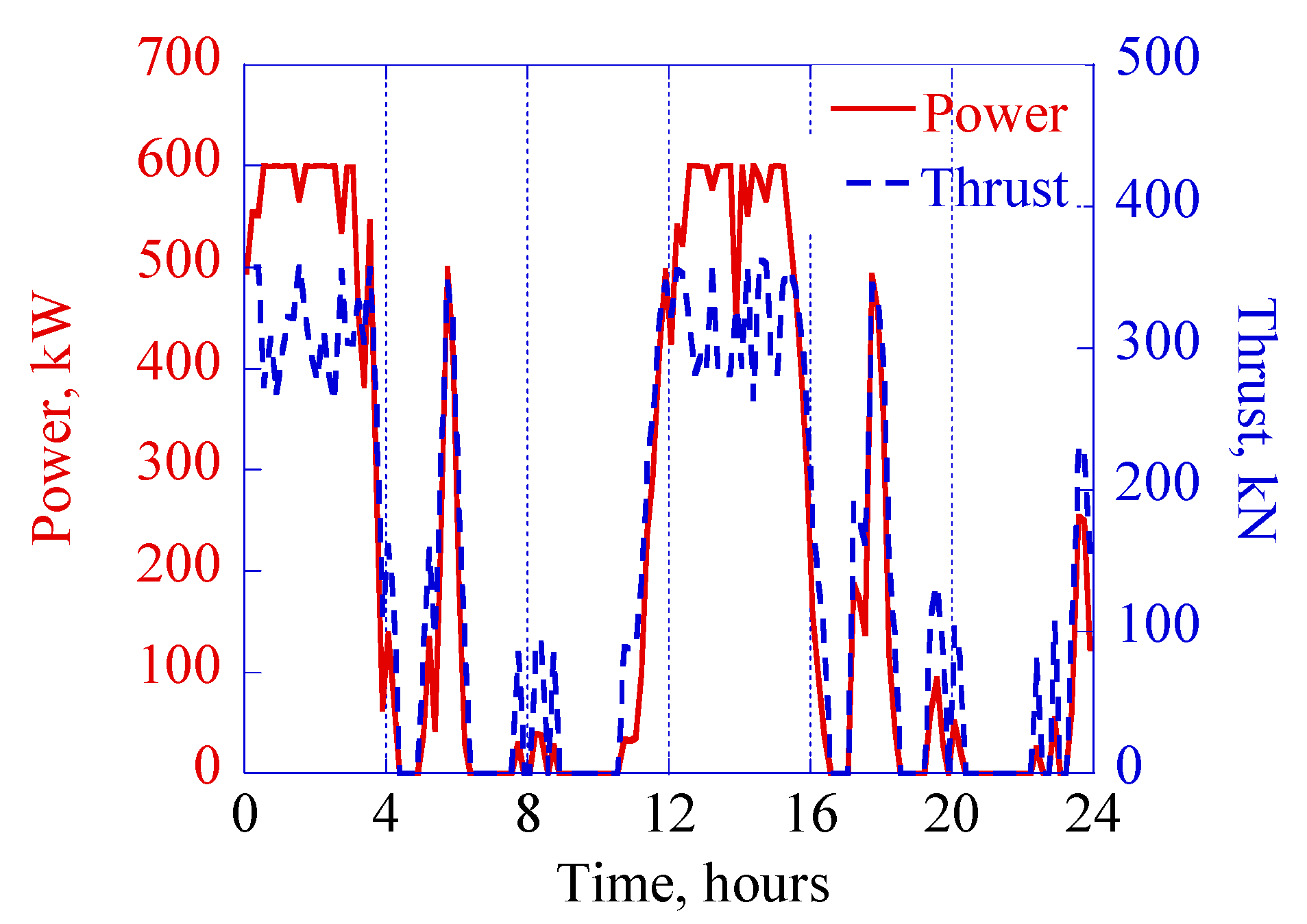The values of the parameters appearing in the formula for F_r have been described previously in Section 4.2; substituting them into the formula results in F_r = 27.6 kN. Comparing the calculated value of the radial load with the values of the thrust shown in Figure 4, it can be seen that the radial load on the main bearing is much smaller than the axial load. Thus, a rolling bearing that is capable to support high axial load along with radial load is needed. A spherical roller bearing suits this requirement. An additional advantage of this type of rolling bearing is that it tolerates misalignment of the shaft relative to the housing and shaft deflection during operation. According to the shaft diameter and estimated axial and radial loads a spherical roller bearing 23,244 CC [34] has been selected for the main bearing in this example. It has the following characteristics: bore diameter d = 220 mm, outside diameter D = 400 mm and basic dynamic load rating C = 2360 kN.

Performance of a rolling bearing is characterised by its basic rating life L₁₀, which is bearing fatigue life associated with 90% reliability expressed in 10⁶ revolutions (e.g., [35])

$$L_{10}={\left(\frac{C}{P}\right)}^p$$

(13)

where P is the dynamic equivalent load and p the load-life exponent (=10/3 for roller bearings). The dynamic equivalent load is estimated by combining axial and radial loads as

$$P=X{F}_r+Y{F}_a$$

(14)

where X is the dynamic radial load factor and Y the dynamic axial load factor; for 23,244 CC X = 0.67 and Y = 2.9 [34]. The trust and, subsequently, the axial load F_a vary with time (see Figure 4). In this case, P in Equation (13) can be replaced by a mean effective bearing load, P_m [35]

$$P_m={\left(\frac{1}{N_r}\underset{0}{\overset{N_r}{\int }}{P}^{p}d{n}_r\right)}^{1/p}$$

(15)

where N_r is the total number of revolutions in one load cycle. Since the rotational speed of the rotor is constant this formula is equivalent to:

$$P_m={\left(\frac{1}{t}\underset{0}{\overset{t}{\int }}{P}^{p}d\tau \right)}^{1/p}$$

(16)

where t is the duration of one load cycle, which can be taken as 24 h (for simplicity, seasonal variations in tidal current velocity are not considered in this example). Equation (16) was integrated numerically using the results for the axial trust shown in Figure 4 that yielded P_m = 820 kN.

The rating life, Equation (13), accounts only for fatigue failure of a properly manufactured rolling bearing, which operates under conventional operating conditions, i.e., when the bearing is properly mounted, protected from foreign matter, adequately lubricated and not exposed to extreme temperature or excessive loads [36]. However, the actual operating conditions of a bearing may differ from the conventional ones. Poor lubrication, contamination, misalignment, shock and vibration, overheating and overload—all these and some other factors may cause premature failures (i.e., earlier than predicted by Equation (13)), whose mechanisms are different from that of rolling contact fatigue. Possible rolling bearing failure modes and their mechanisms are well documented in [37].

To account for the possible failure modes, Equation (3) for the failure rate of a rolling bearing, λ_RB, can be expressed in the following form [10]:

$${\lambda }_{RB}={\lambda }_{RB,B}{C}_{\nu }{C}_C{C}_T{C}_{SF}{C}_M$$

(17)

where λ_RB,B is the base failure rate, C_ν is the influence factor for lubricant, C_C the influence factor for contamination, C_T the influence factor for operating temperature, C_SF the influence factor for operating service conditions, and C_M takes into account model uncertainty. Since the selected bearing 23,244 CC is tolerant to misalignment the corresponding influence factor is not taken into account. It is estimated that the operating temperature of the main bearing does not exceed 100 °C; in such conditions C_T = 1 [10] and, therefore, may be excluded from further consideration.

As should be clear from the previous discussion, λ_RB,B represents the fatigue failure mode and, therefore, should be related to L₁₀. The latter is derived from the distribution of the rolling bearing fatigue life, which is described by a Weibull distribution [35]:

$$R\left(t\right)=\exp \left[-{\left(\frac{t}{\theta }\right)}^{\alpha }\right]$$

(18)

where θ is the characteristic life and α the Weibull slope; for roller bearings, it is recommended to use α = 9/8 [35]. According to the definition of L₁₀, there is the following relationship between the latter and the characteristic life:

$$\theta =\frac{L_{10}}{{\left(-\ln 0.9\right)}^{1/\alpha }}=\frac{L_{10}}{0.1353}$$

(19)

The average failure rate is the reciprocal of the mean time to failure (MTTF) [7], i.e., λ_RB,B = 1/MTTF, while for the Weibull distribution MTTF = θΓ(1/α + 1), where Γ(.) is a gamma function. For α = 9/8, Γ(1/α + 1) = 0.9580 that leads to λ_RB,B = 0.1412/L₁₀. To take into account various uncertainties associated with the determination of λ_RB,B (in particular, with the determination of L₁₀), the latter will be treated as a lognormal random variable with a mean equal to 0.14/L₁₀ and COV = 0.20.

The influence factor for lubricant, C_ν, can be estimated as [10]:

$$C_{\nu }={\left(\frac{{\nu }_1}{\nu }\right)}^{0.54}$$

(20)

where ν is the actual kinematic viscosity of the lubricant at the operating temperature and ν₁ the reference kinematic viscosity required to obtain adequate lubrication condition. For rotational speed ω < 1000 rpm, the latter can be calculated as [36]:

$${\nu }_1=\mathrm{45,000}{\omega }^{-0.83}{d}_m^{-0.5}$$

(21)

where d_m = 0.5(d + D) is the mean bearing diameter in mm. For the main bearing considered in the example ν₁ = 286 mm²/s. The lubrication condition is characterised by the viscosity ratio κ = ν/ν₁. The higher κ, the smaller C_ν and the lower the failure rate, i.e., the longer the bearing life. However, the viscosity ratio should not exceed 5 because of increased friction losses at higher values of κ. Lubricant viscosity decreases exponentially with increasing operating temperature. Therefore, C_ν is very sensitive to the operating temperature of the main bearing, which may vary significantly over the turbine operating time. It is estimated that the operating temperature varies between 20 °C and 100 °C with a mean of 60 °C. This variability of the operating temperature is described by a beta distribution with COV = 0.20. For illustrative purposes, a synthetic lubricant of ISO VG 1500 class with VI = 160 is selected for the main bearing. The relationship between the kinematic viscosity (in mm²/s) of this lubricant and the operating temperature (in °C), T_o, can be approximately described by the following formula:

$$\nu \left(T_o\right)=\mathrm{10,000}\exp \left(-0.048T_o\right)$$

(22)

The influence factor for contamination takes into account both water and particle contamination and is expressed as [12]:

$$C_C=1.176\times {0.21}^{0.01-cw}{\left(FR\right)}^{0.25}$$

(23)

where c_w is the percentage of water in the lubricant and FR the oil filter rating in μm (it is assumed that FR = 20 μm). The percentage of water in the lubricant is treated as a random variable. It is assumed that it can be described by a beta distribution defined on the interval (0.01,1) with mean 0.2% and COV = 0.30.

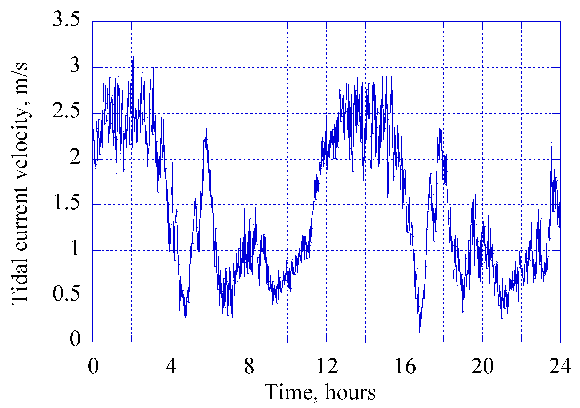
The influence factor for operating service conditions accounts for a negative effect of shock and vibration on the failure rate of a rolling bearing. As can be seen from Figure 2, there is significant turbulence of tidal flow that causes shock loads and possible vibrations of the main bearing. Thus, C_SF is modelled as a beta random variable defined on (1, 3) [10] with a mean of 1.5 and COV = 0.20. C_M is treated exactly in the same way as in the evaluation of the failure rate of the main seal.

Initially, the prior distributions of the failure rate of the main bearing were generated for the three different values of COV_CM and their lognormal approximations were found. These results are presented in Figure 10, while the main characteristics of the prior estimates of the failure rate are shown in

Table 3. Characteristics of prior and posterior (after one calendar year of operation) distributions of the failure rate of the main bearing.

COVCM	nf (Failures)	μλRB (pmh)	COVλRB	λRB,0.05 (pmh)	λRB,0.95 (pmh)
0.1	prior distribution
	−	13.5	0.46	5.9	25.4
	posterior distribution
	0	13.3	0.46	5.9	24.8
	1	16.1	0.46	7.1	30.2
	2	19.5	0.46	8.6	36.2
	3	23.5	0.45	10.5	43.7
0.3	prior distribution
	−	13.5	0.56	4.9	27.8
	posterior distribution
	0	13.2	0.55	4.9	27.0
	1	17.2	0.55	6.5	35.1
	2	22.4	0.54	8.5	45.4
	3	29.0	0.54	11.0	58.6
0.5	prior distribution
	−	13.5	0.71	3.8	31.5
	posterior distribution
	0	13.0	0.69	3.8	30.1
	1	19.2	0.68	5.7	44.1
	2	28.2	0.67	8.4	64.2
	3	41.0	0.66	12.4	92.3

. Similar to the corresponding results for the main seal, an excellent agreement can be observed between the generated prior distributions and their lognormal approximations. To illustrate the effects of updating, first, four possible outcomes of the bearing operating during one calendar year—no failure, one, two and three failures, were considered. The updated values of μ_λ,RB, COV_λ,RB, λ_RB,0.05 and λ_RB,0.95 are presented in Table 3. Similar to the corresponding results for the main seal, the information that one bearing has operated without failures for one year does not change significantly the failure rate estimates compared to their prior values. However, if the main bearing fails during one year the updated values of its failure rate become noticeably higher and the uncertainty interval much wider, in particular when belief in the prior estimate is weak (i.e., COV_CM = 0.5). The results obviously also depend on the number of failures over the one-year period.

Second, the effect of operating without failures of the main bearing of several identical HATTs (up to 20) during one calendar year was considered. The posterior distributions of the failure rate were derived using Equation (7), where t was equal to the number of the turbines. Using these posterior distributions, values of μ_λ,RB, λ_RB,0.05 and λ _RB,0.95 were estimated. Results of the analysis are shown in Figure 11. According to the results, if belief in the prior estimate is strong or medium (i.e., COV_CM ≤ 0.3) updating leads to relatively small changes in the failure rate characteristics. However, if belief in the prior estimate is weak then the use of the new information becomes more beneficial. The results demonstrate the importance of selecting a value of COV_CM. They show that this value should depend not only on existing data and knowledge about the performance of the mechanical component in other operating and environmental conditions but also on the availability of new reliability data related to the performance of this component in tidal stream turbines. If a large amount of such data is expected to become available within a relatively short period of time then a high value of COV_CM may be set to benefit more from these new data. However, if new data are scarce (e.g., obtained from testing a single prototype device) then more efforts need to be put into the validation and quantification of a prior model in order to increase our confidence in this model and reduce the value of COV_CM. The selection of COV_CM needs to be re-assessed as new data become available. If there is a noticeable difference between the observed number of failures and the expected one in accordance to the prior distribution, this may indicate that the model used to derive the prior does not take into account all possible failure modes and/or the influence factors do not fully cover the effects of actual operating and environmental conditions. As a result, the degree of belief in the prior model needs to be re-considered and then either the model should be modified or COV_CM increased.

Regarding the frequency of the failure rate updating, for mechanical components like the main seal and main bearing with the expected failure rate of the order of 10⁻⁵ pmh, it can be recommended this is carried out annually, like in the case studies presented above. Taking into account the bathtub curve for failure rates (e.g., [9]), it is expected that initially the failure rate of a component will be converging to its actual expected value. A steady increase of the failure rate over time will indicate that the component has reached its wear-out stage. At this stage, the proposed approach can still be used (with constant updating of the failure rate) or, if there are enough data, a time-dependent model of the failure rate can be introduced. However, modelling of the failure rate at this stage is not that important from a practical point of view because if there is an indication of wear, the component should be replaced rapidly.

5. Conclusions

A modified method of the influence factors for the assessment of the failure rates of mechanical components of a PTO system of tidal stream turbines has been presented. The method enables various uncertainties associated with the determination of the influence factors and the method itself to be accounted for. Using a Bayesian approach, the method also allows combining generic failure data for similar components from other industries with new information from observing the performance of the components in operating tidal stream turbines. A case study illustrating the application of the method has been provided. The probabilistic evaluation of the failure rates of two components of the PTO system of a HATT—main seal and main bearing—was considered. It has been shown how probabilistic models (or deterministic values) of the influence factors can be derived in accordance with the specific operating and environmental conditions of a HATT. Special attention has been paid to updating the initial/prior estimates of the failure rates, when new information about the performance of the components in operating HATTs becomes available. In particular, it has been shown that the factor representing uncertainty associated with the method (in the context of a Bayesian approach, it can also be interpreted that this factor represents the degree of belief in the method and its results) has a major influence on results of the updating. It has been suggested that the coefficient of variation (COV) of this factor should be selected in relation to the amount of new data on the component performance, which become available for the assessment. If a large amount of such data is expected to be available, a relatively high value of the COV (say, 0.5 or higher) should be selected to gain more benefit from these data. Finally, the proposed method can be applied not only to tidal stream turbines but for the reliability assessment of devices in any new technology, which includes mechanical components used previously in other technologies.

References

1. IEA. Offshore Wind Outlook 2019, International Energy Agency. Available online: https://www.iea.org/reports/offshore-wind-outlook-2019 (accessed on 27 July 2021).
2. IRENA. Innovation Outlook: Ocean Energy Technologies; International Renewable Energy Agency: Abu Dhabi, United Arab Emirates, 2020; Available online: https://www.irena.org/publications/2020/Dec/Innovation-Outlook-Ocean-Energy-Technologies (accessed on 12 October 2021).
3. Encarnacion, J.I.; Johnstone, C.; Ordonez-Sanchez, S. Design of horizontal axis tidal turbine for less energetic current velocity profiles. J. Mar. Sci. Eng. 2019, 7, 197. [Google Scholar] [CrossRef] [Green Version]
4. Energy Roadmap 2050. Available online: https://ec.europa.eu/energy/sites/ener/files/documents/2012_energy_roadmap_2050_en_0.pdf (accessed on 27 July 2021).
5. Magagna, D.; Uihlein, A. Ocean energy development in Europe: Current status and future perspectives. Int. J. Mar. Energy 2015, 11, 84–104. [Google Scholar] [CrossRef]
6. Bucher, R.; Jeffrey, H.; Bryden, I.G.; Harrison, G.P. Creation of investor confidence: The top-level drivers for reaching maturity in marine energy. Renew. Energy 2016, 88, 120–129. [Google Scholar] [CrossRef] [Green Version]
7. SINTEF and NTNU. OREDA Handbook 2015: Offshore and Onshore Reliability Data, 6th ed.; SINTEF and NTNU: Gjøvik, Norway, 2015. [Google Scholar]
8. Delorm, T.M.; Zappala, D.; Tavner, P.J. Tidal stream device reliability comparison models. Proc. Inst. Mech. Eng. Part O J. Risk Reliab. 2011, 226, 6–17. [Google Scholar] [CrossRef]
9. Modarres, M.; Kaminskiy, M.; Krivtsov, V. Reliability Engineering and Risk Analysis: A Practical Guide; CRC Press: New York, NY, USA, 1999. [Google Scholar]
10. NSWC-10. Handbook of Reliability Prediction Procedures for Mechanical Equipment; Naval Surface Warfare Center, Carderock Division: West Bethesda, MA, USA, 2010.
11. Wolfram, J. On assessing the reliability and availability of marine energy converters: The problems of a new technology. Proc. Inst. Mech. Eng. Part O J. Risk Reliab. 2006, 220, 55–68. [Google Scholar] [CrossRef]
12. Iliev, C.; Val, D. Tidal current turbine reliability: Power take-off train models and evaluation. In Proceedings of the 3rd International Conference on Ocean Engineering, Bilbao, Spain, 6–8 October 2010; pp. 1–6. [Google Scholar]
13. Ewing, F.J.; Thies, P.R.; Shek, J.; Bittencourt Ferreira, C. Probabilistic failure rate model of a tidal turbine pitch system. Renew. Energy 2020, 160, 987–997. [Google Scholar] [CrossRef]
14. Han, L.; Wang, Y.; Zhang, Y.; Lu, C.; Fei, C.; Zhao, Y. Competitive cracking behavior and microscopic mechanism of Ni-based superalloy blade respecting accelerated CCF failure. Int. J. Fatigue 2021, 150, 106306. [Google Scholar] [CrossRef]
15. Lu, C.; Fei, C.-W.; Feng, Y.-W.; Zhao, Y.-J.; Dong, X.-W.; Choy, Y.-S. Probabilistic analyses of structural dynamic response with modified Kriging-based moving extremum framework. Eng. Fail. Anal. 2021, 125, 105398. [Google Scholar] [CrossRef]
16. Keshtegar, B.; Bagheri, M.; Fei, C.-W.; Lu, C.; Taylan, O.; Thai, D.-K. Multi-extremum modified response basis model for nonlinear response prediction of dynamic turbine blisk. Eng. Comput. 2021, 1–12. [Google Scholar] [CrossRef]
17. Han, L.; Chen, C.; Guo, T.; Lu, C.; Fei, C.; Zhao, Y.; Hu, Y. Probability-based service safety life prediction approach of raw and treated turbine blades regarding combined cycle fatigue. Aerosp. Sci. Technol. 2021, 110, 106513. [Google Scholar] [CrossRef]
18. Lu, C.; Fei, C.-W.; Liu, H.-T.; Li, H.; An, L.-Q. Moving extremum surrogate modeling strategy for dynamic reliability estimation of turbine blisk with multi-physics fields. Aerosp. Sci. Technol. 2020, 106, 106112. [Google Scholar] [CrossRef]
19. Val, D.V.; Iliev, C. Reliability of power train components in tidal stream turbines. In Proceedings of the 11th International Conference on Applications of Statistics and Probability in Civil Engineering (ICASP11), Zurich, Switzerland, 26 July 2011. [Google Scholar]
20. Williams, M.M.R.; Thorne, M.C. The estimation of failure rates for low probability events. Prog. Nucl. Energy 1997, 31, 373–476. [Google Scholar] [CrossRef]
21. Thies, P.R.; Smith, G.H.; Johanning, L. Addressing failure rate uncertainties for marine energy converters. Addressing failure rate uncertainties of marine energy converters. Renew. Energy 2012, 44, 359–367. [Google Scholar] [CrossRef] [Green Version]
22. Mosleh, A.; Apostolakis, G. The assessment of probability distributions from expert opinions with an application to seismic fragility curves. Risk Anal. 1986, 6, 447–461. [Google Scholar] [CrossRef]
23. MIL-HDBK 217F. Reliability Prediction of Electronic Equipment; United States Department of Defense: Washington, DC, USA, 1991.
24. Doyle, R.L. Mechanical reliability. In Handbook of Reliability Engineering and Management, 2nd ed.; Ireson, G., Coombs, C.F., Moss, R.Y., Eds.; McGraw-Hill: New York, NY, USA, 1995; pp. 19.1–19.27. [Google Scholar]
25. DNV GL. DNVGL-ST-0164: Tidal Turbines; DNV GL: Bærum, Norway, 2015. [Google Scholar]
26. Fraenkel, P. Marine current turbines: Pioneering the development of marine kinetic energy converters. Proc. Inst. Mech. Eng. Part A J. Power Energy 2007, 221, 159–169. [Google Scholar] [CrossRef]
27. Somers, D.M. The S814 and S815 Airfoils; Airfoils Inc.: Pennsylvania, PA, USA; State College: Pennsylvania, PA, USA, 1992. [Google Scholar]
28. NREL. NWCT Engineering Tools (AeroDyn). Available online: https://www.nrel.gov/wind/nwtc/aerodyn.html (accessed on 27 July 2021).
29. Drela, M. XFoil: An Analysis and Design System for Low Reynolds Number Airfoils. In Proceedings of the Conference on Low Reynolds Number Aerodynamics, Indiana, IN, USA, 5–7 June 1989; University of Notre Dame: Indiana, IN, USA, 1989. [Google Scholar]
30. Mott, R. Machine Elements in Mechanical Design; Prentice Hall: London, UK, 2006. [Google Scholar]
31. Netzel, J.P.; Freimanis, I. Performance and wear testing of mechanical seals in sea water service. Lubr. Eng. 1999, 55, 15–19. [Google Scholar]
32. Lebeck, A.O. Principles and Design of Mechanical Face Seals; John Wiley & Sons: New York, NY, USA, 1991. [Google Scholar]
33. Summers-Smith, J.D. (Ed.) Mechanical Seal Practice for Improved Performance; Mechanical Engineering Publications: London, UK, 1992. [Google Scholar]
34. SKF Interactive Engineering Catalogue. Available online: http://www.skf.com (accessed on 27 July 2021).
35. Harris, T.; Kotzalas, M. Essential Concepts of Bearing Technology; Taylor & Francis: New York, NY, USA, 2007. [Google Scholar]
36. ISO 281:2007. Rolling Bearings—Dynamic Load Ratings and Rating Life; International Standard Organisation: Geneva, Switzerland, 2007. [Google Scholar]
37. Tallian, T.E. Failure Atlas for Hertz Contact Machine Elements, 2nd ed.; ASME: New York, NY, USA, 1999. [Google Scholar]
Figure 1. Reliability block diagram of power take-off (PTO) system.
Energies 14 06586 g001
Figure 2. Tidal current velocity versus time at the horizontal axis tidal turbine’s (HATT) site.
Energies 14 06586 g002
Figure 3. Power and thrust versus current speed.
Energies 14 06586 g003
Figure 4. Power and thrust versus time.
Energies 14 06586 g004
Figure 5. Loads acting on the low-speed shaft.
Energies 14 06586 g005
Figure 6. General arrangement of mechanical face seal: 1—seal faces; 2—secondary seals; 3—face loading elements (spring, bellows).
Energies 14 06586 g006
Figure 7. Generated prior distributions of the seal failure rate and their lognormal approximations.
Energies 14 06586 g007
Figure 8. Prior and posterior (after one calendar year) distributions of the seal’s failure rate: (a) COVCM = 0.1; (b) COVCM = 0.3; (c) COVCM = 0.5.
Energies 14 06586 g008
Figure 9. Prior and posterior (after one calendar year) distributions of the seal’s failure rate for arrays of HATTs (COVCM = 0.5): (a) nf = 0; (b) nf = 1.
Energies 14 06586 g009
Figure 10. Generated prior distributions of the bearing failure rate and their lognormal approximations.
Energies 14 06586 g010
Figure 11. Change of the failure rate characteristics when a number of HATTs operate without failure of the main bearing during one calendar year.
Energies 14 06586 g011