Economic Dispatch of Power Retailers: A Bi-Level Programming Approach via Market Clearing Price

Abstract

For power retailers in a smart grid, it is necessary to design an economic dispatch method to maintain a balance between power supply and demand on the sale side as well as obtain better economic benefits. This study concentrates on the economic dispatch of the dominant retailer in a regional market. The dominant retailer is considered to be equipped with generator resources such as distributed photovoltaics (PV), wind turbines (WT), and microturbines (MT). As one retailer cannot exactly predict the market conditions of other retailers, the retail market is considered to be modeled as a dichotomous-market model consisting of the dominant retailer market and the other retailers market. As a result, a bi-level optimal dispatch model is proposed for the dominant power retailer based on the dichotomous-market model. In the proposed model, the outer problem aims to minimize the costs of purchases under time-of-use (TOU) price given in the market clearing process, while the inner problem is formulated to simulate the process of market clearing. Furthermore, the bi-level model is converted to a single-level model via the Karush–Kuhn–Tucker (KKT) conditions and eventually solved by employing the YALMIP toolbox with Gurobi solver. Finally, a case study is conducted to validate the effectiveness and adaptability of the proposed model, and the analysis of the variables is presented.

1. Introduction

The economic dispatch problem of the smart grid has been of considerable interest in the power system academia in recent years [1]. The study of economic dispatch in power systems involves microgrids [2], virtual plants [3], renewable energy [4], battery storage systems (BSS) [5], power retailers [6], demand response (DR) [7,8], etc. Moreover, with the further development of the power industry, modern power systems have been transformed to be far more complex, characterized with high renewable energy penetrations, distributed facilities, and advanced metering and communication technologies, as well as ever-increasing customer risk awareness. These new trends bring participants tremendous challenges, especially for power retailers [9] that lie between the supply side and the demand side.

As proposed by the French economist François Perroux in [10], all markets, including the electricity market, can be structurally divided into perfect competition and incomplete competition markets. The difference between these two categories of markets is whether the prices can be influenced by suppliers and/or customers [11,12]. In electricity markets, the presence and absence of different elements such as DR and renewable energy can lead to fluctuations in electricity prices [13], and these phenomena are more evident in regional markets. For instance, in the retail markets in China, a number of power retailers established by the state grid will play a dominant role in the regional markets in the next few years. In [14,15,16], it is presented that significant difference appears in the market operations of retailers with different qualifications in countries and regions such as the UK, Singapore, Northern Europe, and the US. As a result, it is valuable to study the economic dispatch of dominant retailers in regional markets. In order to maintain the dominant role, power retailers are willing to own generation resources. Such generation resources can be derived from retailers’ self-owned generating units, sale-side aggregated distributed power, and aggregators’ purchasable resources. Additionally, these generation resources enable dominant retailers to have economic dispatch capabilities in a region.

The trading behavior of retailers can be summarized as two types of contracts, one with the supply side and the other with the demand side, which is commonly described as a bi-level Stackelberg-based model [17]. These bi-level models can be divided into two main categories depending on the different participants in the game. One is the game between retailers and customers [18], and the other is between retailers and the energy market [1,19,20]. In [18], a bi-level model is proposed to determine the optimal interplay between the retailer’s tariff design and the prosumer’s decisions regarding using the storage, consumption, and electricity purchases from as well as electricity sales to the grid. In [1], a pricing strategy in the smart grid is analyzed by modeling the economic dispatch problem as a bi-level game in the electricity market, including the wholesale market and the retail market. However, the impacts of the uncertainty and the renewable energy consumption are not involved in [1,18]. In [19], a two-stage stochastic programming scheme is modeled to cope with the uncertainty, and both the participation of retailers in the day-ahead market and impacts of DR are taken into account. In [17], a bi-level Stackelberg-based model between an electricity retailer and consumers is presented, in which the upper level consists of a price-maker retailer (PMR) modeled as the leader who seeks to maximize its own profit by adopting optimal pricing strategies.The lower level of the model consists of four followers, three of them represent customer groups with distinct reactions to DR programs, and their objective function is defined as minimizing the cost of purchased electricity while preserving the welfare level. The fourth follower is the electricity pool, which is responsible for the implementation of market mechanisms and determination of market clearing price (MCP), with the aim of increasing the consumers’ welfare. However, these kind of models are based on the assumption that information is completely knowable, which is challenging to realize in practice.

Given that one retailer cannot exactly anticipate the market conditions and decision making of other retailers in a regional market, a dichotomous-market model is proposed in this study, which contains the dominant power retailer market and other retailers market. In this dichotomous-market model, the dominant retailer reduces operating costs while satisfying customers’ demands with dispatchable resources such as microturbines (MT), distributed photovoltaics (PV), wind turbines (WT), etc. These dispatchable resources can be considered either self-built by the dominant retailer or aggregated from the demand side. In this process, the uncertainty brought by renewable energy consumption is represented by random variables and confidence levels, which reflect the retailer’s tolerance to cope with risk. In contrast, other retailers are modeled as passive recipients of prices, as for one retailer, it is unable to predict their decision-making and market conditions accurately. Considering the problem of distributed renewable energy consumption, uncertainties faced by the dominant retailer in a given region, and the impacts of retailers’ day-ahead economic dispatch on the market clearing process, a bi-level model between retailers, market, and customers is proposed.

The main contributions of this paper are as follows:

• In the proposed dichotomous-market model, a regional retail market containing the dominant retailer and other retailers is constructed through market share.
• A bi-level model based on the dichotomous-market model is proposed for scenarios where the decision making of other retailers in the market is unavailable, and its advantages are explored in Section 3.
• Apart from the effect of economic dispatch on the clearing price, the effect of different confidence levels and renewable energy consumption rate (indicate risk tolerance for retailers) has been taken into consideration, which are discussed in the numerical case.

The rest of this paper is organized as follows. A bi-level optimal scheduling model for the dominant power retailer is proposed in Section 2, as well as the models of uncertain variables, such as load and PV output, along with chance-constrained programming, are carried out. Afterwards, the proposed dispatch model is numerically verified in Section 3. Finally, the conclusions are drawn in Section 4.

2. Main Results

2.1. Problem Formulation

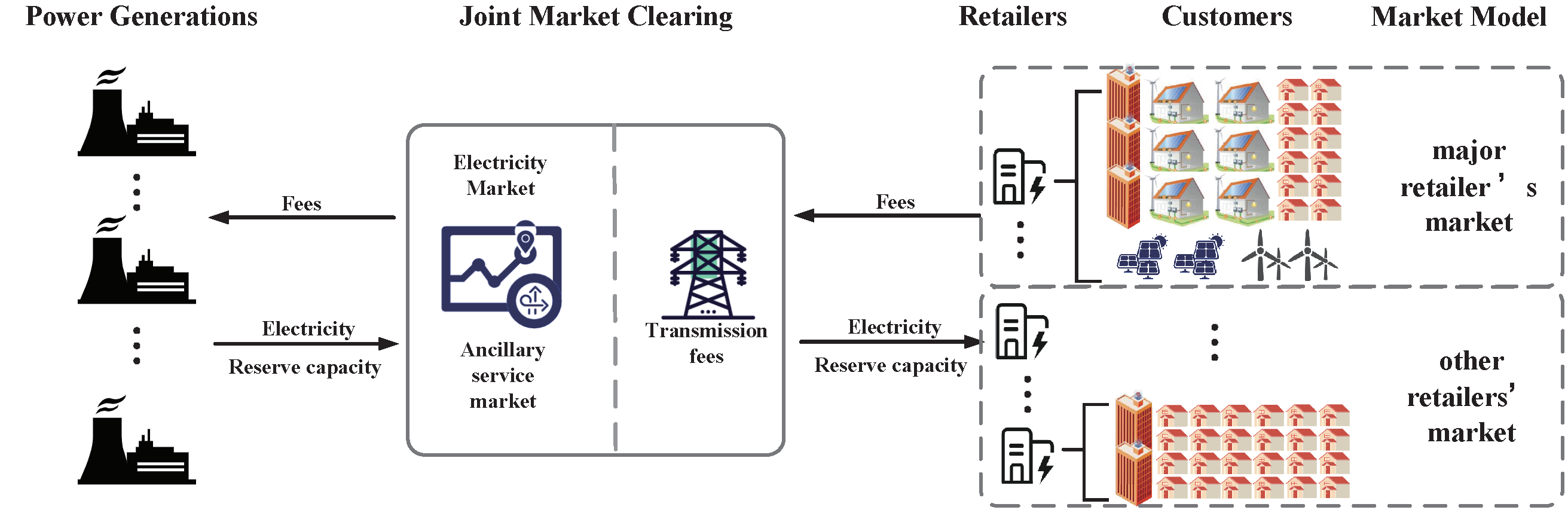
In this section, the concrete content of the dichotomous market is presented in Figure 1. Additionally, the construction of the bi-level model is introduced. To begin with, the dichotomous market proposed in this study consists of two parts: (1) the dominant retailer market and (2) the other retailers market. According to the current retail markets in China, a number of power retailers established by the state grid have been playing a dominant role in the regional markets. The operations of dominant retailers differ significantly from that of ordinary retailers in that the actions of the dominant retailer have an impact on MCP, while the common retailers are price recipients. The economic dispatch model in this paper is proposed for the dominant retailers with dispatching capabilities, as illustrated in the concept of incomplete competition market, where the decisions of such retailers have an impact on prices. However, the other retailers in the given region are aggregated into the other part in the model, referred to as “the other retailers’ market”, considered to be passive recipients of prices. Distinguished with many existing studies, the behavior of other retailers is modeled to be the passive reception of prices, which is from the perspective of one retailer rather than the whole market. It is consistent with reality because the behavior of the various participants in the market is difficult to accurately predict.

Based on the dichotomous market, the behavior of retailers can be described in a bi-level model. On the demand side, the dominant retailer is required to satisfy customers’ electricity demand within its service and undertake the task of renewable energy consumption. To obtain better purchasing costs, the dominant retailer can dispatch self-built resources (such as microturbines (MT), distributed photovoltaics (PV), wind turbines (WT), etc.) in addition to purchasing power and reserve on energy and auxiliary markets. These dispatchable resources can be considered either self-built by the dominant retailer or aggregated from the demand side. As a result, the outer problem of the bi-level model is constructed to obtain an optimal purchase cost with market clearing price (MCP) for the dominant retailer. The inner problem is to model the joint market clearing process of the energy and auxiliary markets. The electricity and reserve in the whole market should be considered in the market clearing process. However, for the dominant retailer, it can only know information about its own customers; therefore, in the proposed model, the whole market demand is modeled by market share, which builds on the assumption that market share shall not change significantly in a short period.

2.2. The Outer Problem

For the dominant retailer, operating costs can be reduced with the economic dispatch of self-built generation resources. The model in this paper takes microturbines (MTs) as an example of controllable generation resources. Apart from controllable generation resources, uncontrollable distributed power resources may be installed within the power sales area, taking WT and PV as examples. To highlight the economics of renewable energy, their operating costs are not included in the outer objective function.

(1) The objective function

Excluding the depreciation and maintenance costs of WT, PV, and MTs, the objective function of the outer problem for a dominant retailer’s day-ahead operating costs, which include the acquisition cost of electricity, the acquisition cost of spare capacity, and the generation cost of gas turbines, follows Equation (1).

$$minf=\sum _{t=1}^T\left. [C_{\mathrm{TR}}\left(P_{\mathrm{TR},t}\right)\mathsf{\Delta }T+C_{\mathrm{R}}\left(U_t,D_t\right)\mathsf{\Delta }T+\sum _{d=1}^{N_{\mathrm{D}}}{C}_{\mathrm{MT}d}\left(P_{\mathrm{MT}d,t}\right)\mathsf{\Delta }T\right]$$

(1)

where $C_{\mathrm{TR}}\left(·\right)$, $C_{\mathrm{R}}\left(·\right)$, and $C_{\mathrm{MT}}\left(·\right)$ denote the electricity purchasing cost, the reserve capacity purchasing cost, and the generation cost of the gas turbine d in hour t, respectively.

The cost of electricity and reserve can be calculated as Equation (2).

$$\begin{array}{c}{C}_{\mathrm{TR}}\left(P_{\mathrm{TR},t}\right)={\gamma }_t{P}_{\mathrm{TR},\mathrm{t}}\\ C_{\mathrm{R}}\left(U_t,D_t\right)={\alpha }_t{U}_t+{\beta }_t{D}_t\end{array}$$

(2)

where $P_{\mathrm{TR},t}$, $U_t$, and $D_t$ are the electricity purchased in the day-ahead (DA) market and the positive and negative reserve resources purchased in the DA ancillary services market in hour t, respectively.

As only considering the cost of MTs, the cost of MTs can be calculated as Equation (3) [21].

$$\sum _{d=1}^{N_{\mathrm{D}}}{C}_{\mathrm{MT}d}\left(P_{\mathrm{MT}d,t}\right)=\sum _{d=1}^{N_{\mathrm{D}}}\left(\frac{C_{\mathrm{nl}}}{L}\times \frac{P_{\mathrm{MT}d,t}}{{\mu }_d}\right)$$

(3)

where $P_{\mathrm{MT}d,t}$ is the active output of microturbine d in hour t, $N_{\mathrm{D}}$ is the number of MTs, $C_{\mathrm{nl}}$ is the price of gas, L represents the calorific value of gas, and ${\mu }_d$ denotes the power generation efficiency of MT d.

(2) Constraint conditions

The equality and inequality constraints in an economic dispatch are as follows.

(a) System power balance constraint. In each dispatch period t, the sum of the power planned to be purchased by retailers in the DA energy market, the WT output, PV output forecast, and the MTs’ active output, ignoring network losses, should equal the load forecast.

$$\sum _{s=1}^{N_S}{P}_{\mathrm{L}fs,t}=\sum _{i=1}^{N_{\mathrm{I}}}{P}_{\mathrm{WT}fi,t}+\sum _{g=1}^{N_{\mathrm{G}}}{P}_{\mathrm{PV}fg,t}+\sum _{d=1}^{N_{\mathrm{D}}}{P}_{\mathrm{MT}d,t}+P_{\mathrm{TR},t}$$

(4)

(b) Reserve constraints.

$$\mathrm{Pr}\left\{U_t+\sum _{d=1}^{N_{\mathrm{D}}}{P}_{\mathrm{MTU}d,t}+\sum _{d=1}^{N_{\mathrm{D}}}{P}_{\mathrm{MT}d,t}+P_{\mathrm{TR},t}\ge \sum _{s=1}^{N_{\mathrm{S}}}{P}_{\mathrm{L}s,t}-\sum _{i=1}^{N_I}{P}_{\mathrm{WT}i,t}-\sum _{g=1}^{N_{\mathrm{G}}}{P}_{\mathrm{PV}g,t}\right\}\ge \eta$$

(5)

$$\mathrm{Pr}\left\{\sum _{d=1}^{N_{\mathrm{D}}}{P}_{\mathrm{MT}d,t}+P_{\mathrm{TR},t}-D_t-\sum _{d=1}^{N_{\mathrm{D}}}{P}_{\mathrm{MTD}d,t}⩽\sum _{s=1}^{N_{\mathrm{S}}}{P}_{\mathrm{L},t}-\sum _{i=1}^{N_I}{P}_{\mathrm{WT}i,t}-\sum _{g=1}^{N_{\mathrm{G}}}{P}_{\mathrm{PV}g,t}\right\}\ge \eta$$

(6)

where $\eta$ is the confidence probability and $P_{\mathrm{MTU}d,t}$ and $P_{\mathrm{MTD}d,t}$ are the positive and negative reserve provided by the MT d in hour t.

(c) MTs constraints.

$$\begin{array}{c}{P}_{\mathrm{MT}d,t}+P_{\mathrm{MTU}d,t}\le P_{\mathrm{MT}dmax}\hfill \\ P_{\mathrm{MT}d,t}-P_{\mathrm{MTD}d,t}\ge P_{\mathrm{MT}dmin}\hfill \\ 0\le P_{\mathrm{MTU}d,t}\le P_{\mathrm{MTU}dmax}\hfill \\ 0\le P_{\mathrm{MTD}d,t}\le P_{\mathrm{MTD}dmax}\hfill \end{array}$$

(7)

where $P_{\mathrm{MT}dmax}$ and $P_{\mathrm{MT}dmin}$ are the upper and lower limits of gas turbine d output. $P_{\mathrm{MTU}dmax}$ and $P_{\mathrm{MTD}dmax}$ are the upper and lower reserve limits that MT d can provide, respectively. Due to the rapid adjustment and small capacity of the MTs’ output, the constraints on the climbing rate of MTs are not considered in this paper.

2.3. The Inner Problem

The inner problem is formulated to simulate the joint clearing process of the energy and auxiliary markets to maximize social welfare. As market clearing is a multi-settlement process containing day ahead (DA) and real time (RT), the proposed model puts more emphasis on the DA schedule to simulate the market clearing process. Ultimately, the DA-scheduled market clearing price for each period in a day can be calculated by making a summation of marginal price and transmission price.

(1) The objective function

The total cost of multi-generators comprises the following two folds: the fuel cost and the spinning reserve cost. To simplify the market clearing model, demand response (load response to price) is ignored [22], and the quotation of the generators is considered to be quoted at cost, which can be formulated as Equation (8).

$$minF=\sum _{t=1}^T\left. [\sum _{i=1}^N{C}_{\mathrm{G}i}\left(P_{\mathrm{G}i,t}\right)\mathsf{\Delta }T+\sum _{i=1}^N{C}_{\mathrm{UR}i}\left(P_{\mathrm{UR}i,t}\right)\mathsf{\Delta }T+\sum _{i=1}^N{C}_{\mathrm{DR}i}\left(P_{\mathrm{DR}i,t}\right)\mathsf{\Delta }T\right]$$

(8)

where $C_{\mathrm{G}i}\left(P_{\mathrm{G}i,t}\right)$, $C_{\mathrm{UR}i}\left(P_{\mathrm{UR}i,t}\right)$, and $C_{\mathrm{DR}i}\left(P_{\mathrm{DR}i,t}\right)$ denote the output cost (quote), positive reserve cost (quote), and negative reserve cost (quote) of the ith generator during time period t, respectively. t stands for the period, and T is the number of periods, which is assumed to be 24 for a DA model; N is the number of generator units in the power system.

The cost quotations contain the output cost, positive reserve cost, and negative reserve cost of the ith generator during time period t. They can be formulated as Equations (9)–(11) [22]:

$$C_{\mathrm{G}i}\left(P_{\mathrm{G}i,t}\right)=a_i{P_{\mathrm{G}i,t}}^2+b_i{P}_{\mathrm{G}i,t}$$

(9)

$$C_{\mathrm{UR}i}\left(P_{\mathrm{UR}i,t}\right)=b_{\mathrm{UR}i}{P}_{\mathrm{UR},t}$$

(10)

$$C_{\mathrm{DR}i}\left(P_{\mathrm{DR}i,t}\right)=b_{\mathrm{DR}i}{P}_{\mathrm{DR}i,t}$$

(11)

where $a_i$, $b_i$, $b_{\mathrm{UDR}i}$, and $b_{\mathrm{DR}i}$ are the quote parameters of generator units.

(2) Constraints

The equality and inequality constraints for the proposed DA market clearing approach are as follows.

(a) System power balance constraint and spinning reserve constraints. In order to maintain the power balance against an outage of the online generator and uncertainties of load forecasts, the controllable spinning reserve (SR) requirement is considered, which is given as Equations (12)–(14).

$$\sum _{i=1}^N{P}_{\mathrm{G}i,t}=P_{\mathrm{Ltotal},t}$$

(12)

$$\sum _{i=1}^N{P}_{\mathrm{UR}i,t}=P_{\mathrm{URtotal},t}$$

(13)

$$\sum _{i=1}^N{P}_{\mathrm{DR}i,t}=P_{\mathrm{DRtotal},t}$$

(14)

where $P_{\mathrm{Ltotal},t}$, $P_{\mathrm{URtotal},t}$, and $P_{\mathrm{DRtotal},t}$ denote the total electricity and positive and negative reserve purchased by all retailers in hour t, respectively; $P_{\mathrm{G}i,t}$, $P_{\mathrm{UR}i,t}$, and $P_{\mathrm{DR}i,t}$ are the bid electricity and positive and negative reserve provided by generator i in hour t.

(b) Generator constraints: The output of each generator is restricted by its minimum and maximum limits and rate constraints.

$$P_{\mathrm{G}i,t}+P_{\mathrm{UR}i,t}\le P_{\mathrm{G}imax}$$

(15)

$$P_{\mathrm{Gi},t}-P_{\mathrm{DR}i,t}\ge P_{\mathrm{G}imin}$$

(16)

$$P_{\mathrm{G}i,t-1}-R_i\mathsf{\Delta }T\le P_{\mathrm{G}i,t}\le P_{\mathrm{G}i,t-1}+R_i\mathsf{\Delta }T$$

(17)

where $P_{\mathrm{G}imax}$ and $P_{\mathrm{G}imin}$ denote the upper and lower output limits of the generator unit i. Additionally, $R_i$ is the climbing rate of unit i.

(c) Spinning reserve constraints. The operating constraints of the spinning reserve, including minimum and maximum limits, are also taken into account, which can be given as Equations (18) and (19)

$$0\le P_{\mathrm{UR}i,t}\le P_{\mathrm{UR}imax}$$

(18)

$$0\le P_{\mathrm{DR}i,t}\le P_{\mathrm{DR}imax}$$

(19)

(3) Market clearing price

The bid-winning electricity and spinning reserve of the generator unit i are obtained through the inner problem. Then, the final market clearing price can be obtained by adding the transmission price, which can be modeled as a constant number $P_{\mathrm{Tr}}$. The final market clearing price can be formulated as follows:

$$P_{\mathrm{L},t}={\lambda }_{\mathrm{L},t}+P_{\mathrm{Tr}}$$

(20)

$$P_{\mathrm{UR},t}={\lambda }_{\mathrm{UR},t}+P_{\mathrm{Tr}}$$

(21)

$$P_{\mathrm{DR},t}={\lambda }_{\mathrm{DR},t}+P_{\mathrm{Tr}}$$

(22)

where the left-hand side of the equation are the final market clearing price of electricity ($P_{\mathrm{L},t}$) and positive and negative reserve ($P_{\mathrm{UR},t}$ and $P_{\mathrm{DR},t}$), while the right-hand side is the marginal price (${\lambda }_{\mathrm{L},t}$, ${\lambda }_{\mathrm{UR}}$, and ${\lambda }_{\mathrm{DR},t}$) obtained through the lower-level optimization.

2.4. Uncertainty Modeling

The uncertainty variables considered in the proposed model include PV, WT, and load. For instance, the PV output is mainly dependent on the amount of solar irradiance reaching the ground, temperature, and characteristics of the PV module itself, as shown in previous studies [23,24]. However, the given bi-level model emphasizes the hourly characteristics, considering the climbing rate of the unit. Distinguished from commonly used probabilistic models, a model established on prediction and bias is applied instead.

On top of this, the PV output can be described as follows, which contains both day and night parts:

$$\sum _{g=1}^{N_{\mathrm{G}}}{P}_{\mathrm{PV}g,t}=\left\{\begin{array}{c}0,nighttime\hfill \\ \sum _{g=1}^{N_G}{P}_{\mathrm{PV}fg,t}+{\epsilon }_{\mathrm{PV},t},daytime\hfill \end{array}\right.$$

(23)

where $P_{\mathrm{PV}g,t}$ denotes the output of the gth PV in time period t, and $N_{\mathrm{G}}$ is the number of PV. In this way, PV output can be expressed as the sum of the output prediction ($P_{\mathrm{PV}gf,t}$) and the bias prediction (${\epsilon }_{\mathrm{PV},t}$) in the daytime, while it comes to 0 in the nighttime. ${\epsilon }_{\mathrm{PV},t}$ denotes the bias prediction in time period t, which obeys a normal distribution with mean 0, and its standard deviation is approximated by Equation (24) [25]:

$${\sigma }_{\mathrm{PV},t}=0.2\sum _{g=1}^{N_{\mathrm{G}}}{P}_{\mathrm{PV}fg,t}+0.02\sum _{g=1}^{N_{\mathrm{G}}}{P}_{\mathrm{PVN}g}$$

(24)

where $P_{\mathrm{PVN}g}$ denotes the installed PV capacity for unit g.

The wind power output is also described in the same way as Equations (25) and (26):

$$\sum _{i=1}^{N_I}{P}_{\mathrm{WT}i,t}=\sum _{i=1}^{N_I}{P}_{\mathrm{WT}fi,t}+{\epsilon }_{\mathrm{WT},t}$$

(25)

$${\sigma }_{\mathrm{WT},t}=0.2\sum _{g=1}^{N_{\mathrm{G}}}{P}_{\mathrm{WT}\mathrm{f}i,t}+0.02\sum _{g=1}^{N_{\mathrm{G}}}{P}_{\mathrm{WT}i}$$

(26)

Similarly, the load within the business of the retailer can be expressed as follows:

$$P_{\mathrm{L},t}=P_{\mathrm{L}fs,t}+{\epsilon }_{\mathrm{L},t}$$

(27)

where $P_{\mathrm{L}fs,t}$, ${\epsilon }_{\mathrm{L},t}$ denote the forecast load and forecast bias in time period t, respectively. ${\epsilon }_{\mathrm{L},t}$ obeys a normal distribution with mean 0 and standard deviation ${\sigma }_{\mathrm{L},t}$. Additionally, ${\sigma }_{\mathrm{L},t}$ can be described in Equation (28) [26], and the coefficient k is normally taken as 1:

$${\sigma }_{\mathrm{L},t}=k{P}_{\mathrm{L}fs,t}/100$$

(28)

2.5. Chance Constraints

Chance constraint programming (CCP), proposed by Charnes and Cooper [27], is a stochastic programming method used to solve problems where the constraints contain random variables, and decisions must be made before the realization of the random variables is observed. Considering that the decision made may not satisfy the constraint when an unfavorable situation occurs, the principle of species is applied: the decision made is allowed not to satisfy the constraint to some extent, but the probability that the constraint holds is not less than a certain confidence level $\alpha$. One of the common forms of CCP can be formulated as follows:

$$\begin{array}{c}maxf\left(x\right)\\ s.t.P_{\mathrm{r}}\left\{g_j(x,\xi )\le 0,j=1,2,\cdots ,k\right\}\ge \alpha \end{array}$$

(29)

where x is an n-dimensional decision vector; $\xi$ is a random vector with known probability density function; $f\left(x\right)$ denotes the objective function; $g_j(x,\xi )\le 0$ represents the random chance constraint function; $P_{\mathrm{r}}\left(·\right)$ represents the probability of an event; and $\alpha$ is the given confidence level.

The chance constraints posed by random variables with uncertainty, such as wind, PV, and load, can be transformed into deterministic constraints. Equations (5) and (6) can be translated into a standard form [28].

$$\mathrm{Pr}\left\{h_1\left(x_1\right)\ge f_1\left({\xi }_1\right)\right\}\ge \eta$$

(30)

$$\mathrm{Pr}\left\{h_2\left(x_2\right)⩽f_2\left({\xi }_2\right)\right\}\ge \eta$$

(31)

where x is the decision variable to be sought, i.e., $U_t$, $D_t$, $P_{\mathrm{MTU}d,t}$, $P_{\mathrm{MTD}d,t}$, and $\xi$ are random variables. ${\xi }_1$ follows a normal distribution with mean ${\sum }_{s=1}^{N_{\mathrm{S}}}{P}_{\mathrm{L}s,t}-{\sum }_{i=1}^{N_I}{P}_{\mathrm{WT}i,t}-{\sum }_{g=1}^{N_{\mathrm{G}}}{P}_{\mathrm{PV}g,t}$ and variance ${\left({\sigma }_{L,t}\right)}^2+{\left({\sigma }_{\mathrm{WT},t}\right)}^2+{\left({\sigma }_{PV,t}\right)}^2$; ${\xi }_2$ follows a normal distribution with mean ${\sum }_{i=1}^{N_I}{P}_{\mathrm{WT}i,t}+{\sum }_{g=1}^{N_{\mathrm{G}}}{P}_{\mathrm{PV}g,t}-{\sum }_{s=1}^{N_{\mathrm{S}}}{P}_{\mathrm{L},t}$ and variance ${\left({\sigma }_{L,t}\right)}^2+{\left({\sigma }_{\mathrm{WT},t}\right)}^2+{\left({\sigma }_{\mathrm{PV},t}\right)}^2$ [25]. It is converted to a deterministic constrained form employing random variable quantile points.

$$\left\{\begin{array}{c}{h}_1\left(x\right)\ge {\Phi }_1^{-1}\left(\eta \right)\hfill \\ h_2\left(x\right)⩽{\Phi }_2^{-1}\left(1-\eta \right)\hfill \end{array}\right.$$

(32)

where $\Phi \left(·\right)$ denotes the specific normal distribution function of $\xi$.

2.6. The Bi-Level Program and KKT Conditions

Following the general formulation of a bi-level program, the retailer problem can be drawn as:

$$\begin{array}{cc}\hfill \mathit{min}& f\left(P_{\mathrm{TR},t},U_t,D_t,P_{\mathrm{MT}d,t}\right)\hfill \\ \hfill s.t.& \mathrm{Equation}\left(4\right)–\mathrm{Equation}\left(7\right)\hfill \\ \hfill & argminF\left(P_{\mathrm{G}i,t},P_{\mathrm{UR}i,t},P_{\mathrm{DR}i,t}\right)\hfill \\ \hfill & s.t.\mathrm{Equation}\left(12\right)–\mathrm{Equation}\left(22\right)\hfill \end{array}$$

Based on the work in [29], the inner problem can be reformulated as an equivalent system of the Karush–Kuhn–Tucker (KKT) conditions, thus turning a bi-level problem into a single-level one. When it comes to the model solution, the Lagrange function can be solved by applying either Jacobian or the function $kkt\left(·\right)$ in the Gurobi solver. It should be noticed that the objective function in Equation (8) contains a quadratic term as shown in Equation (9), while other terms in the objective function and constraints are all linear ones. The resulting problem can be solved as a single-level problem due to the convexity of both the objective function and the constraints. Problems of this type can be solved by employing the Gurobi solver in YALMIP toolbox.

3. Numerical Results and Discussion

In this section, the methodologies and parameters employed for generating scenarios for the market clearing process and economic dispatch are presented. Furthermore, the role and impact of the MTs, the confidence level of stochastic programming, and the renewable energy consumption rate in the economic dispatch decision of the dominant retailer are discussed separately in the generated scenarios.

3.1. Scenario Generation

In the numerical example presented in this paper, the inner market clearing model contains three power generation units. The quoted and operating parameters of the generating units are shown in

Table 1. The quote parameters of generator units.

Generator Unit i	Electricity Cost Parameters/ $\mathbf{\$}·{\left(\mathbf{MW}·\mathbf{h}\right)}^{-1}$		Reserve Cost Parameters/ $\mathbf{\$}·{\left(\mathbf{MW}·\mathbf{h}\right)}^{-1}$
	${\mathit{a}}_{\mathit{i}}$	${\mathit{b}}_{\mathit{i}}$	${\mathit{b}}_{\mathrm{UR}\mathit{i}}$	${\mathit{b}}_{\mathrm{DR}\mathit{i}}$
1	0.045923	15.47	14.00	13.80
2	0.012800	17.82	18.14	15.34
3	0.010875	12.88	16.18	15.12

and

Table 2. The operating parameters of generator units.

Generator Unit i	Active Output Limits/MW		Reserve Limits/MW		Climbing Rate Limit/ $\mathbf{\$}·{\left(\mathbf{MW}·\mathbf{h}\right)}^{-1}$
	${\mathit{P}}_{\mathbf{G}\mathit{i}max}$	${\mathit{P}}_{\mathrm{G}\mathit{i}min}$	${\mathit{P}}_{\mathbf{UR}\mathit{i}max}$	${\mathit{P}}_{\mathbf{DR}\mathit{i}max}$	${\mathit{R}}_{\mathit{i}}$
1	60	15	3.335	3.335	40.02
2	80	12.5	4.150	4.150	49.80
3	140	25	8.350	8.350	100.20

, which can be referred to in [30].

In the outer dispatch model, the dominant retailer A is used as an example, which has two MTs. For two MTs, the essential parameters are as follows: the price of gas $C_{\mathrm{nl}}=4$ $/MBtu and the calorific value of gas L = 0.0097 MWh/m³, while the operating parameters of MTs are shown in

Table 3. The operating parameters of MTs.

Microturbine Units d	Active Output Limits/ MW		Reserve Limits/MW		Generation Efficiency
	${\mathit{P}}_{\mathbf{MT}\mathit{d}max}$	${\mathit{P}}_{\mathbf{MT}\mathit{d}min}$	${\mathit{P}}_{\mathrm{MTU}\mathit{d}max}$	${\mathit{P}}_{\mathrm{MTD}\mathit{d}max}$	${\mathbf{\mu }}_{\mathit{d}}$
1	4.0	0.2	0.5	0.5	58.7%
2	4.0	0.2	0.5	0.5	60.0%

, which can be referred to in [21]. Furthermore, retailer A faces problems with renewable energy consumption within their service, which usually comes from aggregators and customers’ distributed power generators. The renewable energy is equated as PV with an installed capacity of 9.1 MW and WT with a rated power of 5 MW.

Apart from the dispatchable MTs and the renewable energy that can be selectively consumed as described above, the main business of the electricity retailer is to provide electricity to customers. This part is modeled by the whole market electricity demand and the market share of electricity sales companies. Since the market share fluctuates little in the short term, it can be regarded as a constant, which is set to 30% in this example. In order to cope with fluctuations in power demand, an additional positive and negative spinning reserve is necessary. The coefficient of the positive and negative spinning reserve to power demand is set to 0.02. The forecasted loads in the whole market and PV and WT output for retailer A in each period are shown in Figure 2. In the cost calculation, transmission price is considered, which is taken as 2/3 of the market clearing price [31], thus giving the MTs a cost advantage.

3.2. Analysis of the Dichotomous-Market Model

At the very beginning, the dichotomous-market model is proposed in this study because we suggest that the dominant retailer’s decisions impact the amount of electricity and reserve involved in the market clearing process. To visualize this, a comparison case is presented where the clearing price is not influenced by the retailer’s decision, and all retailers are left to passively accept the price and then make a dispatch action. Thus, the original bi-level model becomes a two-stage model with the market clearing and dispatch processes. To obtain a fair comparison performance, the global parameters market share, confidence level, and the renewable energy consumption rate are set to 30%, 95%, and 100%, respectively. Additionally, a large consumption rate is set to make the results more visible, which are shown as in demand for positive and negative reserves.

In

Table 4. The cost of retailers in four scenarios. Scenario i: two-stage model for a dominant retailer; scenario ii: two-stage model for a common retailer; scenario iii: bi-level model for a dominant retailer; scenario iv: bi-level model for a common retailer.

Scenarios	Electricity Cost $\left(\mathbf{\$}\right)$	Positive Reserve Cost $\left(\mathbf{\$}\right)$	Negative Reserve Cost $\left(\mathbf{\$}\right)$	MTs Cost $\left(\mathbf{\$}\right)$	Total Cost $\left(\mathbf{\$}\right)$
i	26,375.56	1892.05	1831.40	3268.23	33,367.25
ii	32,943.30	611.00	611.00	0	34,165.29
iii	25,595.66	1481.19	1787.88	4395.33	33,260.06
iv	32,636.99	626.13	642.03	0	33,905.15

, retailers are divided into two categories: (1) the dominant retailer, which is equipped with dispatchable resources, and (2) the common retailers, who can only passively accept prices. In the two-stage model, the retailers’ economic dispatch decisions do not affect the simulated market clearing process. As shown in scenario ii and scenario iv, it can be found that the total cost of the common retailer decreases by 0.76%, as the common retailer is classified as other retailers in the dichotomous market due to the perceived lack of access to specific information and can only act as a price recipient. The reduction in costs in two scenarios indicates that the bi-level has a lower clearing price compared with the two-stage model. This result proves that the dispatch of retailers impacts the clearing price, as the dispatching behavior of retailers reduces the amount of electricity participating in the market clearing process, resulting in a lower clearing price. A similar result can be obtained in scenario i and scenario iii, where the total cost of the dominant retailer is reduced by 0.32%. The deterioration in cost reduction performance is due to the increase in reserve costs resulting from renewable energy consumption. Apart from this, a comparative analysis of scenarios i, ii iii, and iv shows that it is not reasonable to ignore the dominant retailer’s dispatching behavior.

3.3. Impact of MTs

In the given model, MT1 and MT2 are set up to undertake part of the power and reserve supply at a lower cost because of the lower transmission fees compared with power plants on the generation side. Given a confidence level of 95% and complete consumption of renewable energy, a discussion on the cost of retailer A in scenarios with and without MTs is presented. The power purchase cost for retailers is shown in

Table 5. Purchasing cost with or without MTs under a confidence level of 95%.

With MTs or Not	Electricity Cost $\left(\mathbf{\$}\right)$	Positive Reserve Cost $\left(\mathbf{\$}\right)$	Negative Reserve Cost $\left(\mathbf{\$}\right)$	MTs Cost $\left(\mathbf{\$}\right)$	Total Cost $\left(\mathbf{\$}\right)$
yes	25,595.66	1481.19	1787.88	4395.33	33,260.06
no	26,485.09	3494.30	3494.30	0	33,473.68

. The partial optimization results in two scenarios are shown in Figure 3 and Figure 4.

(1) Analysis of MTs’ impact on retailer’s day-ahead economic dispatch costs

In Table 5, it can be found that when retailer A is equipped with MTs, although the generation cost of MTs is incurred, the power cost and reserve cost are lower than that where it is not equipped with MTs. MTs reduce the total operating cost and reserve cost of retailer A by 0.64% and 53.22% compared with that where it is not equipped with MTs. The reasons for this phenomenon are as follows:

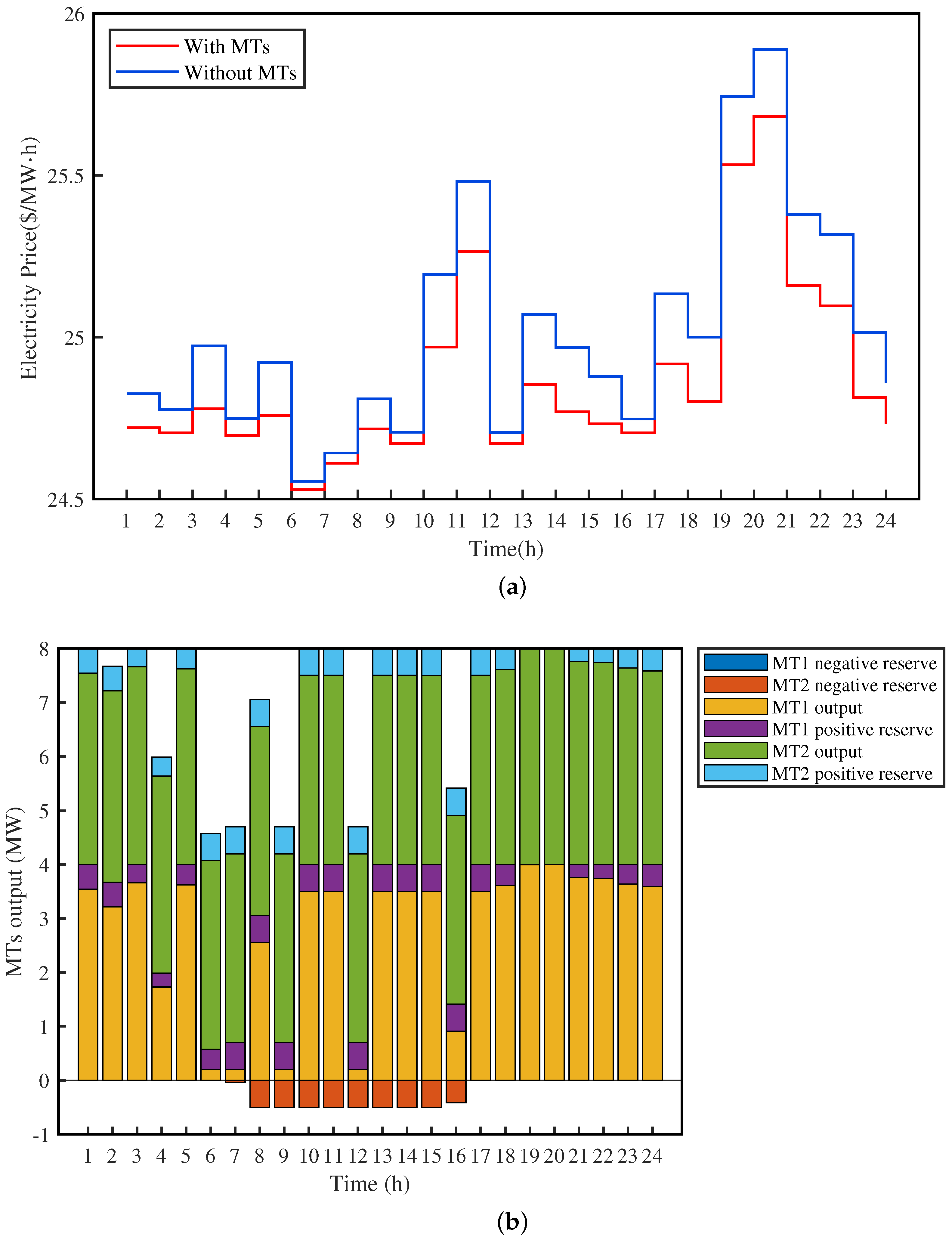
(a) Figure 3a demonstrates the market clearing price in scenarios with and without MTs, and the price has the same double-peak character as the electricity demand. Figure 3b demonstrates the output and reserve planning of MT1 and MT2 in each interval. From Figure 3a,b, it can be observed that MTs’ output increases when the power price is high, which is specifically reflected in the two intervals, 10:00–11:00 and 19:00–20:00. As a result, retailer A’s power purchase during the high-price period is reduced, which is the main reason for the power cost reduction. Additionally, at the same time, it can also be observed that MT2, owing to its lower cost, gives priority to the power output, as shown in Figure 3b.

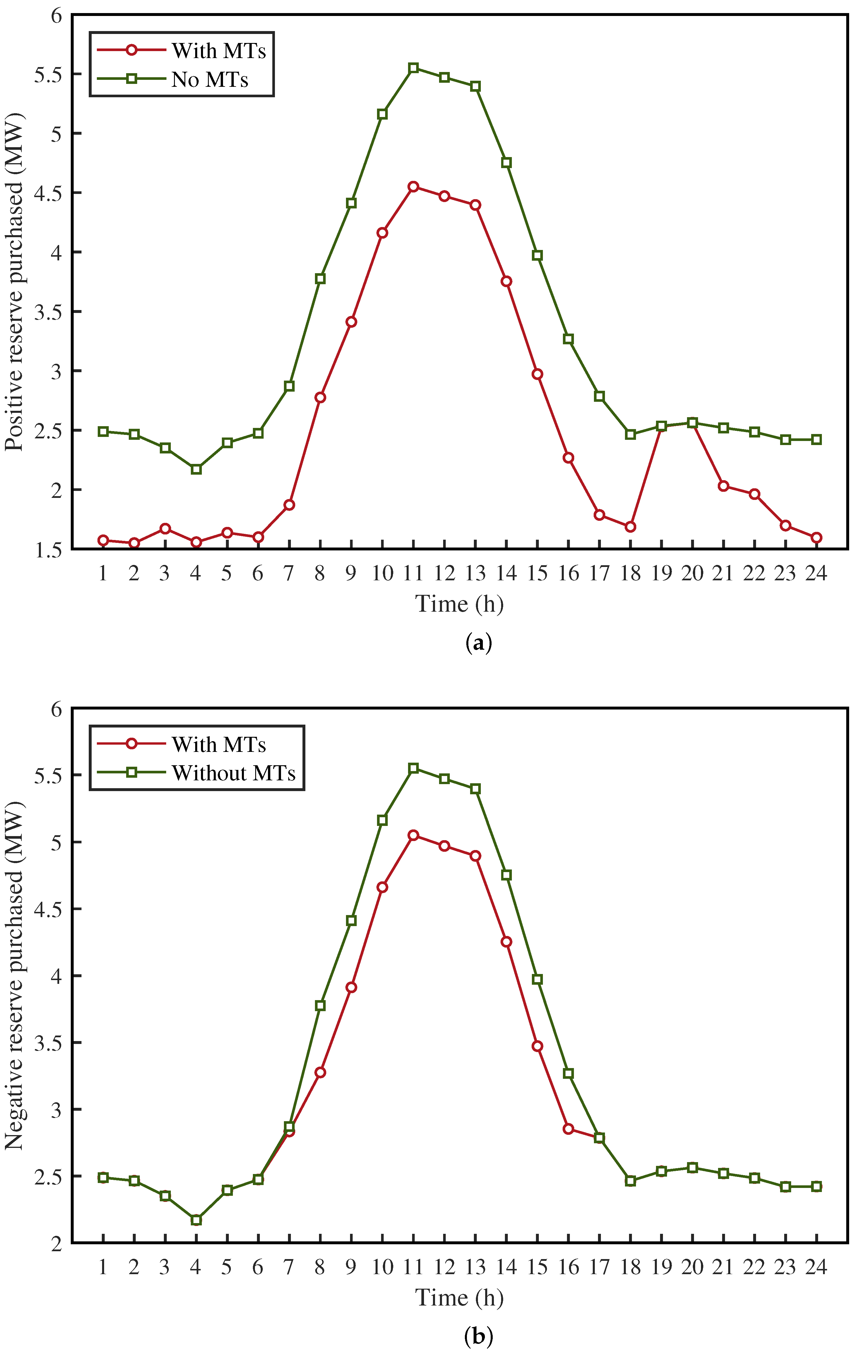
(b) The positive and negative reserve purchased from the auxiliary market is shown in Figure 4. In Figure 4a, it can be observed that MT1 and MT2 prioritize power over the reserve to cope with higher electricity prices between 18:00 and 20:00. During this interval, the positive reserve is provided by the auxiliary market. At other intervals, both MT1 and MT2 arrange positive reserve output, resulting in a reduction in positive reserve purchase from the market. The negative reserve purchase case is similar to the positive reserve. In some intervals, 00:00-6:00 and 17:00–24:00, MTs fail to provide cheap negative reserve as higher negative reserve cost. Furthermore, it is worth noting that reserve demand is related to electricity demand and new energy consumption. As can be seen in Figure 2 and Figure 4, the electricity demand has a double-peak character, while the reserve demand only has a single-peak character. This phenomenon is because the active consumption of renewable energy requires more reserve resources to satisfy the power balance requirements.

(2) Analysis of MTs’ impacts on power clearance price

It can be observed in Figure 3b that the power clearance prices are both high in two cases during the peak load periods, such as 10:00–12:00 p.m. and 19:00–21:00 p.m., because the amount of purchased power is large, and the unit 2 with higher cost needs to join, resulting in a high price.

To conclude, the dispatch schedule of retailers with controllable distributed power sources may have a certain impact on market clearing results, especially during peak load periods; by optimizing the scheduling of controllable distributed power sources (MTs), the operating costs of retailers can be effectively reduced.

3.4. Impact of Confidence Levels and Consumption Rate

For retailer A equipped with MTs, under the chance constraint confidence levels of 98%, 95%, and 91%, the power purchase cost is shown in

Table 6. The cost of electricity purchased by the retailer at $\eta$ of 98%, 95%, and 91%.

Confidence Levels	Electricity Cost $\left(\mathbf{\$}\right)$	Positive Reserve Cost $\left(\mathbf{\$}\right)$	Negative Reserve Cost $\left(\mathbf{\$}\right)$	MTs Cost $\left(\mathbf{\$}\right)$	Total Cost $\left(\mathbf{\$}\right)$
98%	25,687.37	1892.14	2183.45	4500.72	34,263.69
95%	25,595.66	1481.19	1787.88	4395.33	33,260.06
91%	25,488.86	1243.24	1449.27	4337.42	32,518.80

, and the partial optimization results under the three confidence levels are shown in Figure 5, Figure 6 and Figure 7.

(1) Impacts of confidence levels on purchase cost

As the confidence levels increase, it can be observed in Table 6 that the purchase cost of retailer A increases, in which the costs of the positive reserve, negative reserve, and MTs all tend to increase. Additionally, when the confidence level changes from 91% to 98%, the positive reserve cost increases by 52.19% and the negative reserve cost increases by 50.66%, while the MTs cost increases by 3.76%, but the power cost increases by only 0.78%. The reasons for this phenomenon are as follows.

(a) As already pointed out in Section 2.4 and Section 2.5, confidence levels affect the tolerance of constraints that contain random variables ($P_{\mathrm{L},t}$, $P_{\mathrm{WT}i,t}$, and $P_{\mathrm{PV}g,t}$). As the confidence level rises, the constraints become tighter, resulting in increased demand for power and reserve, but the reasons for the increase are different. 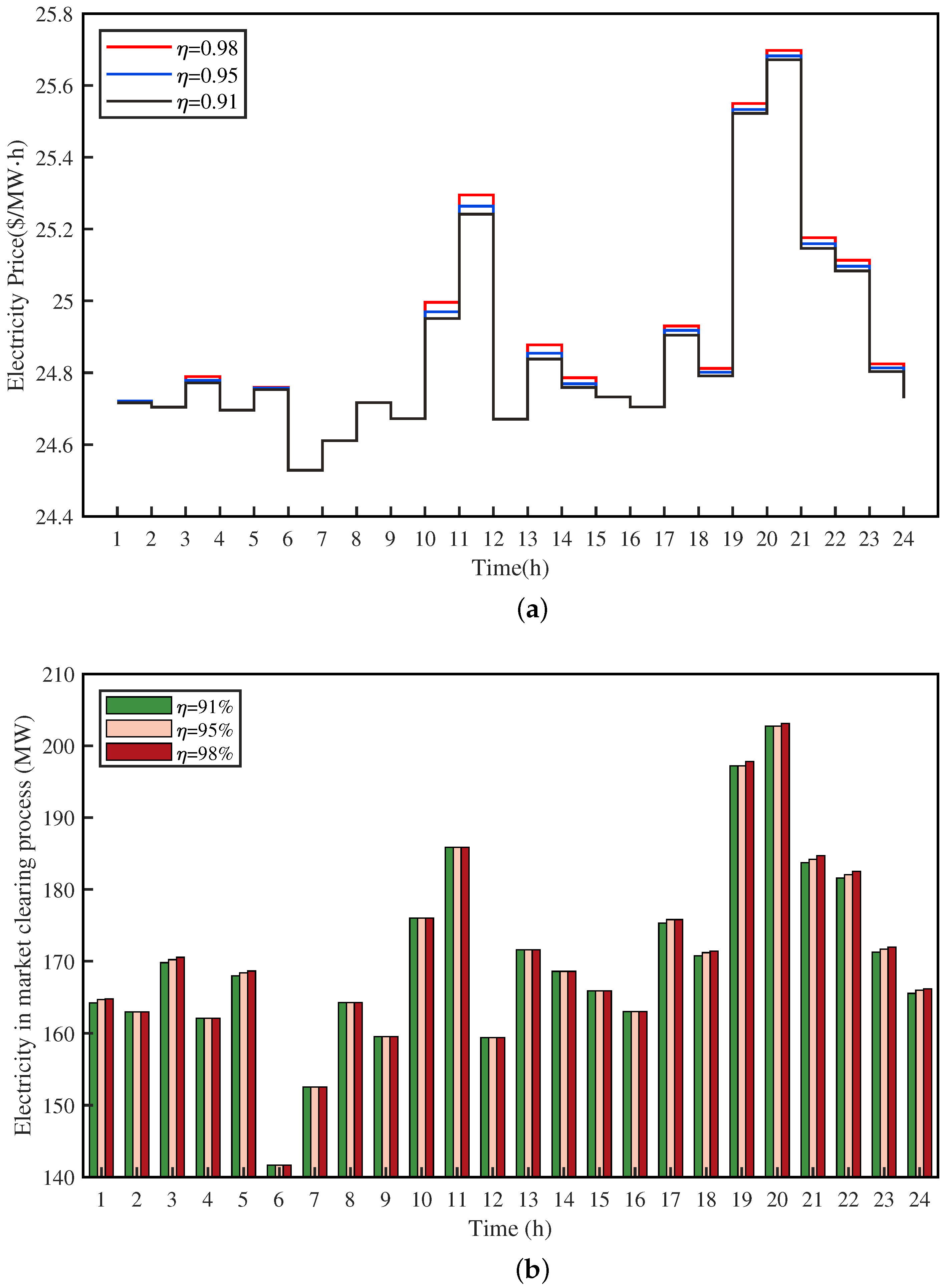For electricity, it is affected by the power balance constraint and the chance constraints (Equations (4)–(6)), while the variation of reserve is mainly reflected in the chance constraints and operating constraints (Equations (5)–(7)). As confidence levels rise, power purchases rise in all intervals (as shown in Figure 5b) and maintain the same double-peak character as power demand. The variation resulted from the chance constraint is small compared with the total demand, so the increase in power purchase cost is not significant.

(b) As shown in Figure 6, the positive and negative reserve purchased by retailer A under three different confidence levels are presented. In comparison with Figure 6a,b, it is evident that the positive and negative reserves do not increase in the same way as the confidence level rises. In Figure 3b, it can be found that the output strategy of MTs is to provide power and positive reserve as a priority, and only in some periods such as 7:00–16:00; MT2 is arranged with negative reserve, which is determined by the cost. As a result, the negative reserve is mainly purchased from the ancillary services market, which is significantly impacted as the confidence level rises. Moreover, MTs’ output strategy reduces the purchase of positive reserve in the auxiliary service market, which is more evident when the confidence level is below 95% (as shown in Figure 3a, in the intervals such as 0:00–6:00, 16:00–18:00, and 20:00–24:00, the increase in confidence level does not affect the purchase of positive reserve.).

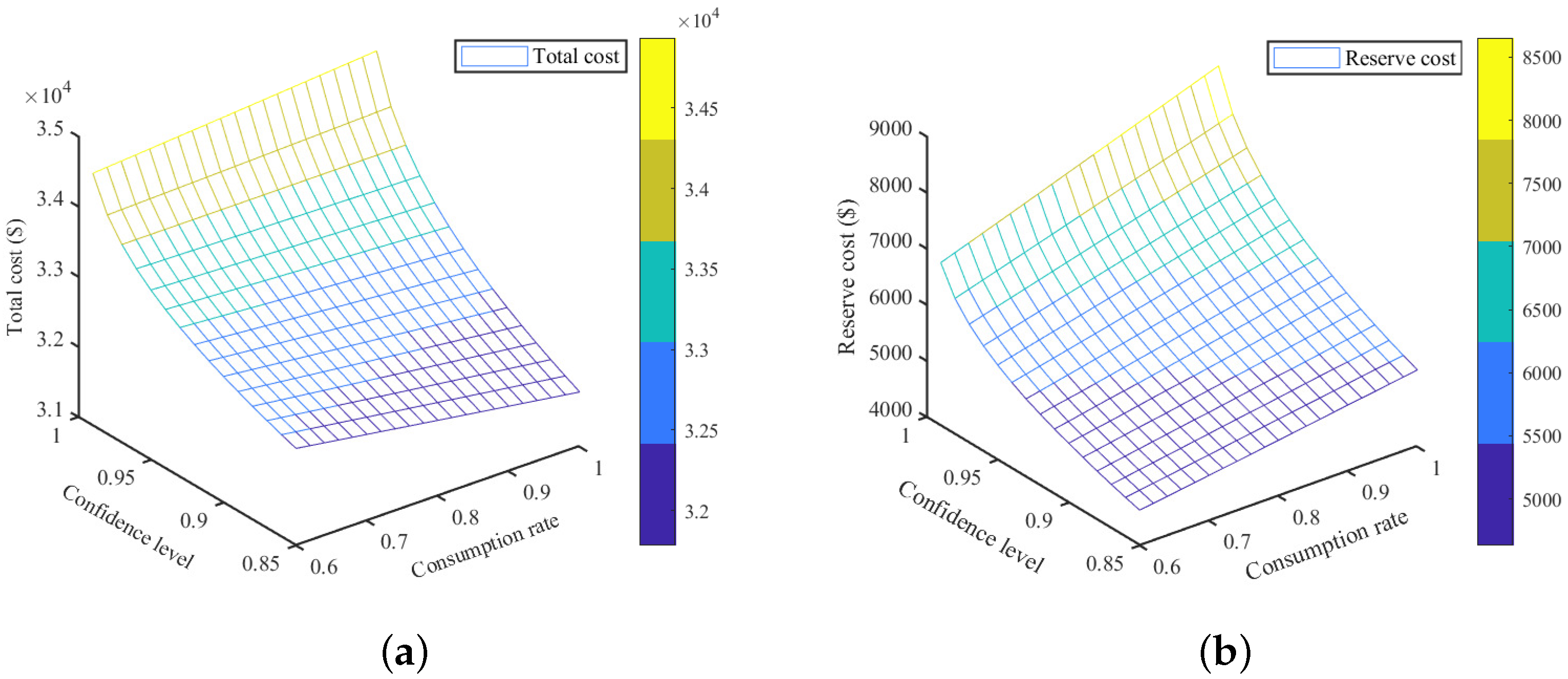
(2) Impacts of consumption rate on purchase cost

Renewable energy consumption affects the balance and chance constraints on electricity consumption, which leads to changes in the amount of electricity and reserve purchases, coupled with the market clearing price. Therefore, in addition to the confidence level discussion, renewable energy consumption’s impact should also be considered. As shown in Figure 7a,b, at the same confidence level, the increase in the consumption rate has different impacts on the total cost and reserve cost. It is worth noting that the total cost contains electricity cost and positive and negative reserve cost, while the reserve cost only contains positive and negative reserves.

Without difficulty, the phenomenon in Figure 7b is that the reserve cost increases as both the confidence level and the consumption rate increase. This is consistent with the intuition that the confidence level and consumption rate increase, the uncertainty becomes more prominent, and the chance constraints tighten, leading to a higher lowerbound on the target value. However, as shown in Figure 7a, it presents a richer connotation due to the incorporation of electricity cost. When the confidence level is low (retailer risk is expected to be low, such as when the confidence level is below 90%), the consumption of more cheap renewable energy contributes to lower total costs. However, when the confidence level is higher (higher risk expectation for retailers, such as when the confidence level is higher than 90%), the consumption of more cheap renewable energy may reduce the electricity cost, while the higher reserve cost will lead to higher total cost instead.

To conclude, the choice of confidence level is related to the risk appetite of the retailer, and a good selection of both confidence level and consumption rate is also essential.

4. Conclusions

In this study, a bi-level model based on the dichotomous market is proposed for scenarios where the decision making of other retailers in the market is unavailable. For a dominant retailer, it is faced with the uncertainty brought by renewable energy consumption, represented by random variables, reflecting the retailer’s tolerance to cope with risk. Additionally, from the case study in Section 3, the conclusion can be drawn in three parts: (1) the impacts of the dominant retailers’ economic dispatching decisions on the whole market shall not be ignored; (2) controllable dispatching resources have good performance in renewable energy consumption scenarios; and (3) a good selection of both confidence levels and consumption rate is essential. However, the dichotomous-market model is created as a last resort. In future research, methods such as power flow analysis, multi-agents, and distributed optimization shall be helpful in studying complex retailer problems.