Article

Performance Simulation of the Active Magnetic Regenerator under a Pulsed Magnetic Field

1
School of Energy and Power Engineering, Huazhong University of Science and Technology, Wuhan 430074, China
2
Wuhan National High Magnetic Field Center, Huazhong University of Science and Technology, Wuhan 430074, China
*
Author to whom correspondence should be addressed.
Energies 2022, 15(18), 6804; https://doi.org/10.3390/en15186804
Submission received: 5 August 2022 / Revised: 11 September 2022 / Accepted: 15 September 2022 / Published: 17 September 2022

Abstract

:
Magnetic refrigeration is acknowledged as a potential substitute for the conventional vapor-compression refrigeration technology, owing to its high efficiency and environmental friendliness. Existing magnetic refrigeration systems are mostly based on permanent magnets, owing to the characteristics of lower magnetic field intensity, non-uniform magnetic field distribution, and lower operating frequency due to the moving parts, which results in a low cooling capacity and small temperature difference. Thus, this study proposes the application of a pulsed magnetic field, with a high intensity and frequency, to a magnetic refrigeration system to achieve a high performance. A verified numerical model is established to investigate the thermodynamic cycle and cooling performance of an active magnetic regenerator (AMR). The transient and steady-state performances of AMR under pulsed and permanent magnetic fields are compared. The results suggest that an AMR can establish a stable temperature difference under a pulsed magnetic field that is 40 times faster than that under a permanent magnetic field. The maximum steady-state cooling capacity under a pulsed magnetic field is 2.5 times that under a permanent magnetic field when the temperature difference is 20 K. Additionally, the effects of pulsed magnetic field waveforms, frequency, and intensity on the performance of AMR are investigated under various utilization factors. These results can guide the improvement of room-temperature magnetic refrigerators.

1. Introduction

It is urgent to develop novel refrigeration technologies to replace the traditional refrigeration technology, due to the increasing energy demand of the refrigeration sector and its increasing contribution to climate change [1]. Room-temperature magnetic refrigeration (RTMR) based on the magnetocaloric effect (MCE) is regarded as a potential alternative to vapor-compression refrigeration, owing to its high efficiency and environmental friendliness [2,3,4].
Since the development of the first RTMR prototype in 1976 [5], there have been more than 70 RTMR prototypes, currently [6,7]. However, RTMR has not been fully commercialized, due to the limited cooling capacity and temperature span of the prototypes. One of the main reasons limiting the performance of prototypes is the limited intensity of the permanent magnet, which is generally lower than 2 T [6]. In addition, the relative motion of permanent magnets and regenerators causes friction loss and system complexity [8]. To address the above problems, Zhang et al. [9] proposed applying pulsed magnets in place of permanent magnets. On the one hand, pulsed magnets can produce high magnetic field intensity, which can fully stimulate the MCE of magnetic materials, thus improving the cooling capacity of prototypes. On the other hand, pulsed magnets can generate magnetic fields that vary over time; therefore, the magnetization and demagnetization of magnetic materials can be realized with no moving parts. Thus, friction losses, flow path, and system complexity caused by the movement are avoided, which can improve the efficiency and reliability of prototypes.
Recently, many scholars have measured the MCE of different magnetic materials under pulsed magnetic fields. Kihara et al. [10,11,12] developed a direct measurement system and measured the adiabatic MCE of Gd and NiCoMnIn in pulsed magnetic fields up to 55 T. The observed adiabatic temperature change (ΔTad) of Gd reached 60 K at 55 T, which is much larger than that at 2 T. Kamantsev et al. [13,14] measured the ΔTad of Gd under different pulsed magnetic field intensities. It showed that ΔTad increased with the field intensity, and the temperature change of Gd can well catch up with the change of pulsed magnetic fields. Ghorbani Zavareh et al. [15] measured the MCE of Gd under different pulsed magnetic field sweep rates (that is, frequency). The results suggested that the MCE of Gd showed inconsiderable changes with magnetic field frequency, which means the MCE of Gd will not be affected even under the high-frequency pulsed magnetic fields. Therefore, the application of high-intensity and frequency-pulsed magnetic fields may be one of the potentially effective solutions to solve the inadequate refrigeration performance of the RTMR prototypes. However, the ultra-high frequency of the pulsed magnetic field poses a challenge to the heat transfer of AMR, the core component of RTMR prototypes [16]; however, there is a lack of research on this issue. Moreover, the effect of the pulsed magnetic field on the refrigeration performance of the AMR is not clear. In this context, the performance of the AMR under a pulsed magnetic field was investigated by numerical simulation in this paper. First, the thermodynamic cycle of an AMR in a pulsed magnetic field was explored. Then, the transient and steady-state performances of AMR under pulsed and permanent magnetic fields were compared. Finally, the influence of characteristic parameters of a pulsed magnetic field on the performance of the AMR was analyzed.

2. Materials and Methods

2.1. Numerical Model Description

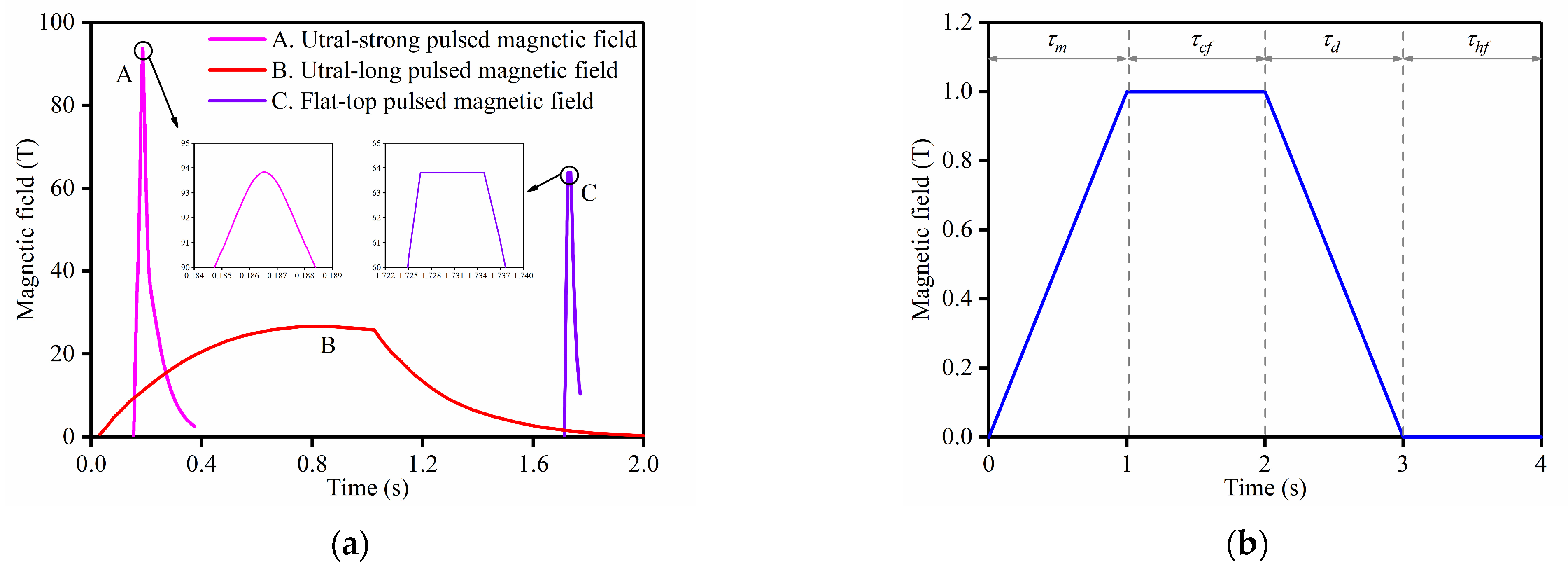
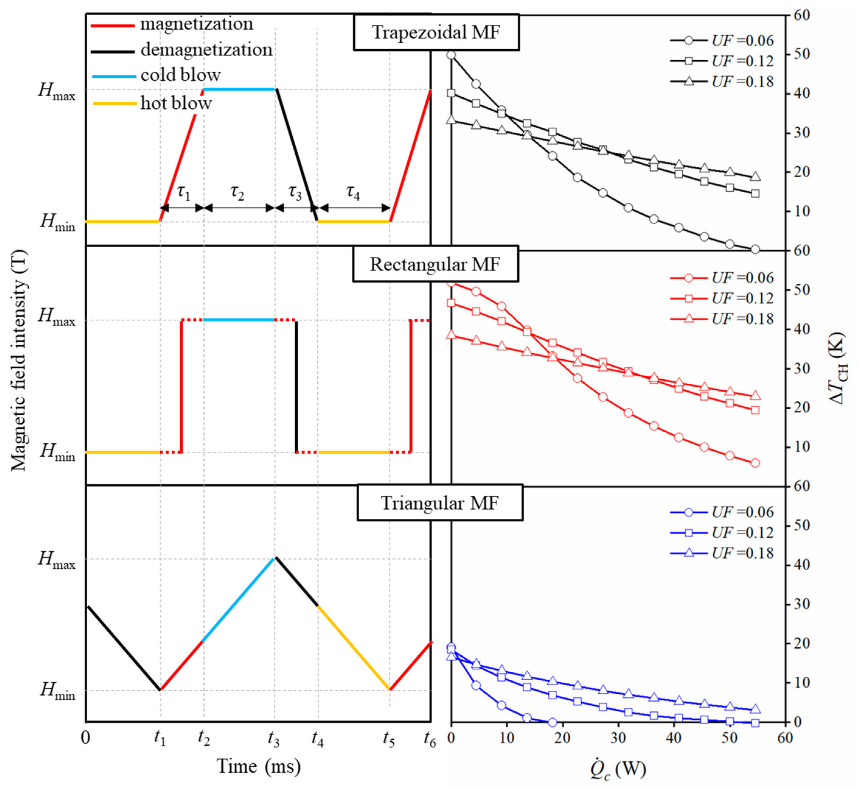
2.1.1. Pulsed Magnetic Field

Pulsed magnetic fields include ultra-strong, ultra-long, and flat-top pulsed magnetic fields, as shown in Figure 1a [17]. Ultra-strong pulsed magnetic fields can reach intensities up to 100 T; however, they have approximately no peak duration, which is required in the classical AMR cycle. Ultra-long pulsed magnetic fields have a second-order pulse width; however, they lack an appropriate peak duration. The profile of flat-top pulsed magnetic fields is similar to that of the magnetic field profile commonly used in the classical AMR cycle, as illustrated in Figure 1b. Thus, it can be applied to the AMR cycle. In contrast to the conventional magnetic field profile, the rise time, fall time, and peak duration of flat-top pulsed magnetic fields are on the order of milliseconds. The extremely short rise and fall times of the magnetic field provide adiabatic conditions for the magnetization and demagnetization of magnetic materials, which reduces adiabatic irreversible losses. However, an extremely short peak duration poses a challenge for the heat transfer. Therefore, the thermodynamic cycle and the performance of the AMR in a flat-top pulsed magnetic field are worth exploring.

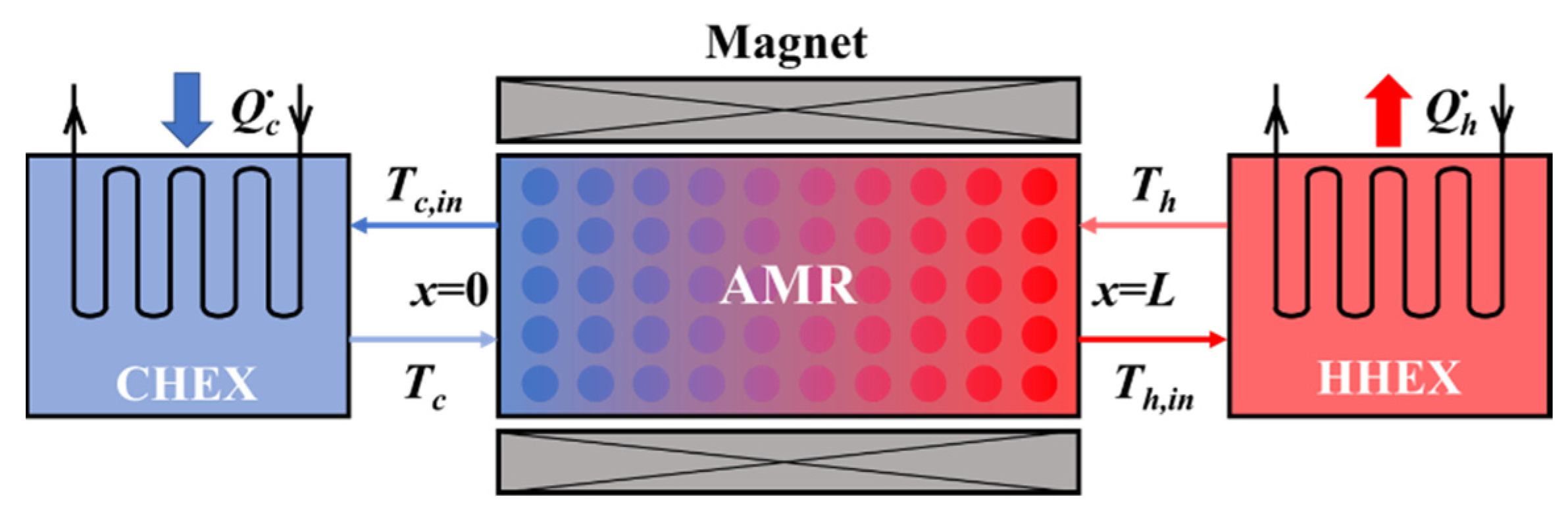
2.1.2. Numerical Model

A schematic diagram of the model is presented in Figure 2, which includes the AMR, magnet, cold-end heat exchanger (CHEX), and hot-end heat exchanger (HHEX).
The AMR is the most important component of the RTMR system and is a porous bed packed with Gd particles in most systems. The 1-D numerical model described by Nakashima et al. [18,19,20] has been widely used to investigate the performance of the AMR and has been validated experimentally. The energy equations for the MCM and heat transfer fluid (HTF) in the AMR can be expressed as:
( 1 ε ) ( ρ c ) s T s t = h e α ( T f T s ) + ( 1 ε ) λ s 2 T s x 2 + ( 1 ε ) ( ρ c ) s ( Δ T a d ) H H t
ε ( ρ c ) f T f t = h e α ( T s T f ) + ε λ f 2 T f x 2 u ε ( ρ c ) f T f x + | u ε p x |
where ε is the porosity of the AMR bed, he refers to the effective heat transfer coefficient. α represents the heat transfer area per unit volume, defined as α = 6(1 − ε)/d, where d is the particle diameter of the MCM. ρ, c, and λ refer to density, specific heat, and heat conductivity, respectively. ΔTad is the adiabatic temperature change of the MCM, and H is the magnetic field intensity. In addition, u and p represent the average fluid velocity and pressure, respectively. The subscripts s and f represent the MCM and HTF, respectively. The items in Equation (1) are the internal energy change of the MCM, heat transfer with the HTF, axial heat conduction, and MCE, respectively. The MCE was expressed as the adiabatic temperature change ΔTad, which is a function of temperature and the magnetic field. The items in Equation (2) represent the internal energy change of the HTF, heat transfer with the MCM, axial heat conduction, advection heat transfer, and viscous dissipation, respectively.
The convective heat transfer coefficient of the HTF and MCM in porous AMR beds was calculated using Equation (3) [21]. Moreover, since the 1-D model neglects the heat conduction in the MCM orthogonal on the flow direction, the convectional heat transfer coefficient was modified by Equation (4) [20].
N u = h d λ f = 2 + 1.1 R e 0.6 P r 1 3
h e = h 1 + B i a 0 = h 1 + h d 2 λ s a 0
where Nu, Re, Pr, and Bi are the Nusselt number, Reynolds number, Prandtl number, and Biot number, respectively. The shape factor a0 depends on the MCM geometry and has a value of 3 for particles.
In addition to the AMR, the CHEX and HHEX are also important components of the RTMR system to ensure the refrigeration function of the system. The HTF absorbs heat from the cold-end space through the CHEX and releases heat to the hot-end environment through the HHEX. The numerical model of CHEX and HHEX was established using the lumped parameter approach [20], as shown in Equations (5) and (6):
m C H E X c f T c t = m f . c f ( T f ( t , x = 0 ) T c ) + Q c .
m H H E X c f T h t = m f . c f ( T f ( t , x = L ) T h ) Q h .
where m, m f . , Q c . , and Q h . are the fluid mass within the heat exchanger, fluid mass flow rate, cooling capacity, and heating capacity, respectively. T f (t, x = 0) and T c are the fluid temperature inflow and outflow of the CHEX in the hot-blow process, respectively. Tf (t, x = L) and Th are the temperatures of the fluid inflow and outflow of HHEX in the cold-blow process, respectively.
According to the flow direction, the boundary conditions can be expressed as:
Cold blow:
T f , x = 0 = T c ;   T f , x = L x = 0
Hot blow:
T f , x = L = T h ;   T f , x = 0 x = 0
MCM:
T s , x = 0 x = 0 ;   T s , x = L x = 0
Frequency ν and utilization factor UF were used to characterize the operating conditions of the AMR.
τ = τ m + τ c f + τ d + τ h f
ν = 1 τ
U F = m ˙ f c f τ c f m s c ¯ s
where τ is the total time of the cycle, τm and τd represent the magnetization and demagnetization times, respectively, and τcf and τhf represent the cold and hot blowing times, respectively.
In addition, the temperature difference ΔTCH between the hot and cold ends of the AMR and cooling capacity Q c . were used to evaluate the performance of the AMR, defined as follows:
Δ T CH = T f , x = L T f , x = 0
Q c . = 1 τ τ d τ d + τ h f m f . c f ( T c T f , x = 0 ( t ) ) d t
In this study, Gd was used as the magnetic refrigerant, and its magnetocaloric properties were obtained using a physical property measurement system and the molecular field theory [22,23], as described in the supplementary material. The time and space steps in the simulation were set to 10−3, and the convergence accuracy was set to 10−6 to ensure that the model could capture the temperature change of the AMR under the fast pulsed magnetic field. The AMR sizes and operating parameters are presented in Table 1.

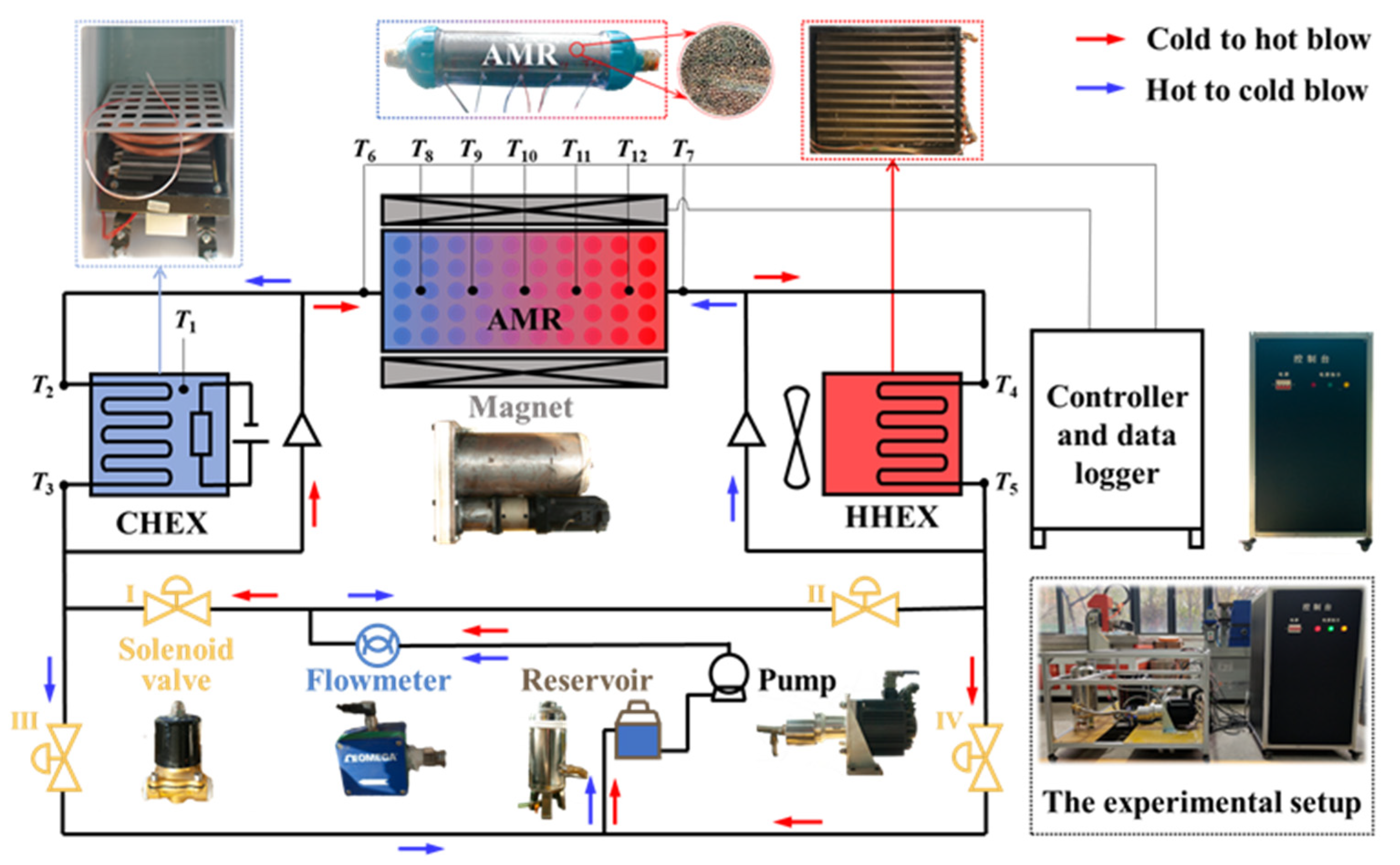
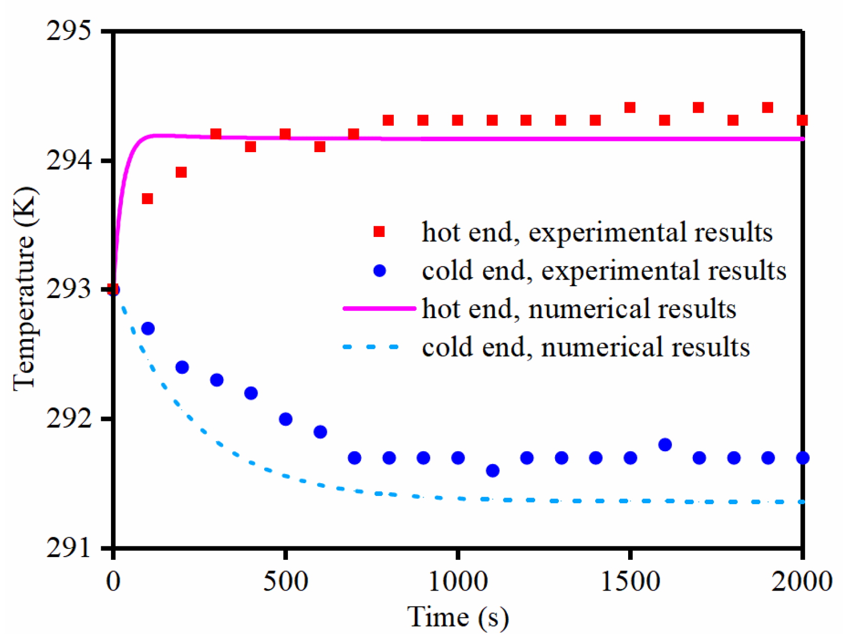
2.1.3. Model Validation

An experimental apparatus was established to verify the numerical model, as illustrated in Figure 3. The AMR bed was a cylinder filled with gadolinium spheres, which was placed in a Halbach magnet. Five T-type thermocouples (TT-T-36-72, accuracy = ±0.5 K) were mounted equidistantly along the AMR, and temperatures were transmitted to the data logger in an interval of 1 s. The CHEX was a coil heat exchanger located in a cabinet with an electrical heater. The HHEX was a finned-tube heat exchanger with a fan. Temperatures of the inlet and outlet of the heat exchangers and cold cabinet were measured using temperature sensors (PT100A, accuracy = ±0.15 K). Water was used as the HTF, and its flow rate was measured using a flowmeter (FMG72B, accuracy = ±0.0009 l/s). A reservoir was used to store the HTF, and the pump delivered oscillatory fluid to the AMR. The flow direction was controlled using four solenoid valves and two check valves. The AMR sizes and operating parameters of experiment are presented in Table 2.
The numerical and experimental results were compared using the hot- and cold-end outlet fluid temperatures of the AMR after hot blowing. Both the numerical and experimental results were based on the parameters listed in Table 1. As demonstrated in Figure 4, the simulated hot-end temperature (i.e., T12) was approximately equal to the experimental value after stabilization, with a maximum error of 0.8%. The simulated cold-end temperature (i.e., T8) was lower than the experimental value, with a maximum error of 3.4%. The deviation between the numerical and experimental values might have been caused by heat leakage losses between the surrounding environment and the AMR. Furthermore, the solenoid valves were significantly heated during the experiments, which caused an increase in the thermal load. Therefore, both the experimental cold- and hot-end temperatures were higher than the simulated values.

3. Results and Discussion

The numerical model was applied to investigate the effects of different factors on the performance of the AMR. First, thermodynamic processes of the AMR cycle were simulated. Subsequently, the performance of the AMR in both pulsed and permanent magnetic fields was investigated. Finally, the effects of fluid mass flow rates and pulsed magnetic field characteristics were investigated. It should be noted that the power consumption required to drive the motion of permanent magnets or the AMR is difficult to be calculated by numerical simulation, as is the power consumption required to generate the pulsed magnetic field and cool the pulsed magnets. Therefore, this paper does not consider the energy consumption of the magnet itself but only explores the thermodynamic cycle and refrigeration performance of the AMR. As a result, the coefficient COP, which characterizes the performance of the system, was not regarded.

3.1. Thermodynamic Cycle

Figure 5 shows the temperature profiles of magnetic material (MCM) at the cold and hot ends of the AMR, where the corresponding pulsed magnetic field waveform is the magnetic field C shown in Figure 1a. Figure 5a demonstrates that the MCM experiences magnetization, heat release (cold blow), demagnetization, and heat absorption (hot blow) in one cycle, which are comparable to those under a permanent magnetic field. Figure 5b shows that after running for several cycles, a periodic steady state was eventually reached, with a ΔTCH established between the hot and cold ends of the AMR, demonstrating the feasibility of pulsed magnetic refrigeration.

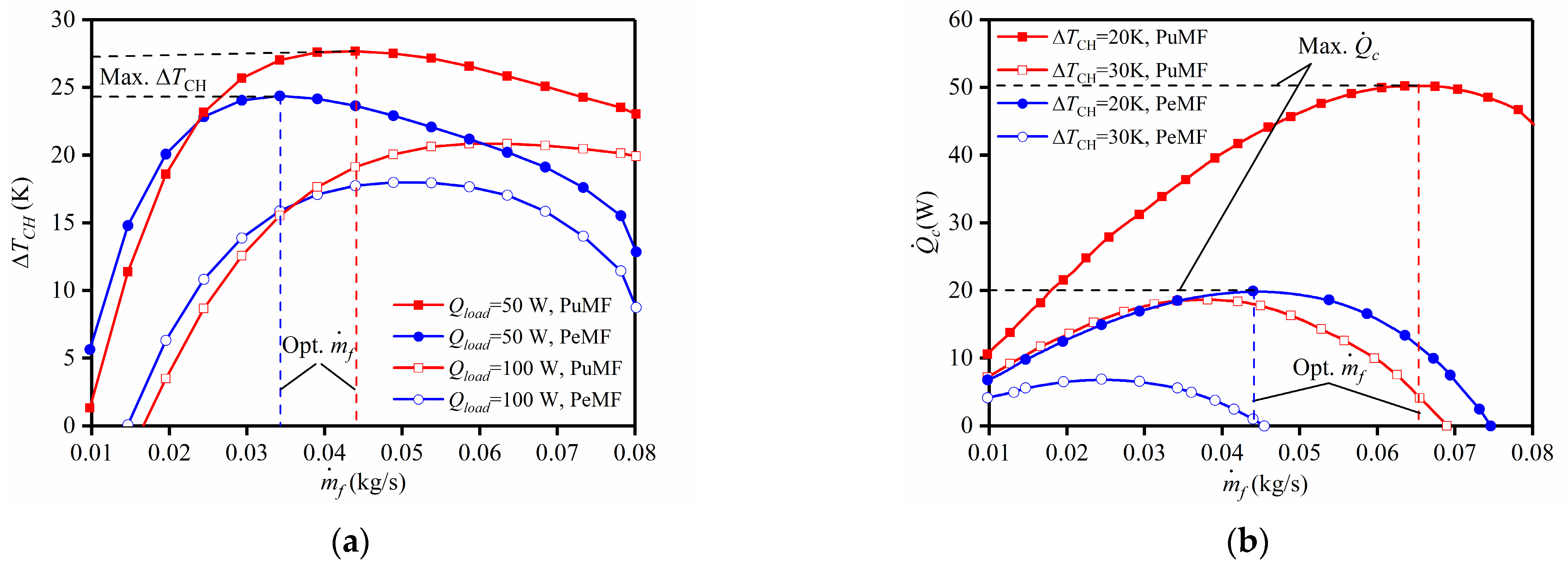
3.2. Comparison of AMR Performance in the Pulsed and Permanent Magnetic Fields

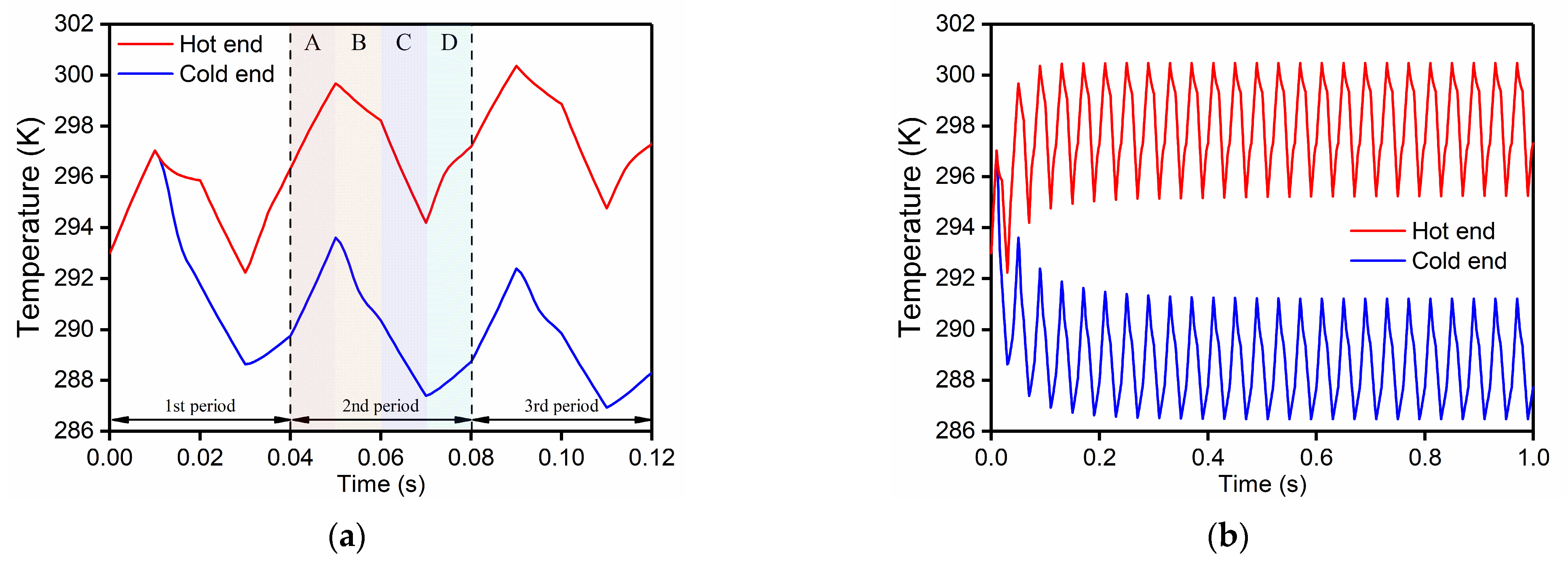
3.2.1. Transient-State Performance

The transient-state performance of the AMR in pulsed and permanent magnetic fields was compared by simulating the transient cold-end temperature (Ts,c) and ΔTCH between the cold and hot ends of the AMR at various UFs, as shown in Figure 6. The corresponding pulsed magnetic field waveform is the magnetic field C in Figure 1a, and the permanent magnetic field waveform is shown in Figure 1b, with the same intensity of 1 T. When the UF was the same, Ts,c decreased faster under the pulsed magnetic field, as did the establishment of ΔTCH. Indeed, both Ts,c and ΔTCH reached steady values in approximately 0.8 s under the pulsed magnetic field, which was 39 times faster than that under the permanent magnet field (i.e., 32 s). This was because the frequency of the pulsed magnetic field was extremely high, and the AMR performed 20 cycles in 0.8 s, which led to a decrease in Ts,c and rapid establishment of ΔTCH. However, the AMR did not complete a cycle under the permanent magnetic field. In addition, Ts,c and ΔTCH stabilized faster with an increase in UF, and the effect of the UF on the stabilization time was more significant in the permanent magnetic field.

3.2.2. Steady-State Performance

The steady-state performance of the AMR in pulsed and permanent magnetic fields was compared by calculating the Q c . and steady ΔTCH at different mass flow rates ( m ˙ f ). As presented in Figure 7, ΔTCH and Q c . in the pulsed and permanent magnetic fields both first increased and then decreased with an increase in m ˙ f . However, optimal m ˙ f values corresponding to the maximum ΔTCH or Q c . were different. Because the pulsed magnetic field had a higher frequency, a larger m ˙ f was required to guarantee the heat transfer. When the cold-end thermal load was 50 W, with an optimal m ˙ f of 0.044 kg·s−1, ΔTCH reached a maximum value of 27.69 K under the pulsed magnetic field, which was 13.6% higher than that in the permanent magnetic field (i.e., 24.37 K). Figure 7b illustrates that Q c . is always larger in the pulsed magnetic field. When ΔTCH was 20 K, with an optimal m ˙ f of 0.065 kg·s−1, the maximum Q c . is 50.24 W in the pulsed magnetic field and was 2.5 times that of the permanent magnetic field (i.e., 19.94 W). In terms of the steady-state Q c . and ΔTC, the performance of the AMR in the pulsed magnetic field was higher than that in the permanent magnetic field.

3.3. Effects of Key Parameters on the Performance of AMR

Because the magnetic field is a vital component of a magnetic refrigeration system, the effects of the pulsed magnetic field parameters must be investigated on the performance of the AMR. Therefore, the effects of three characteristic parameters, including the magnetic field waveform, frequency, and intensity, were investigated.

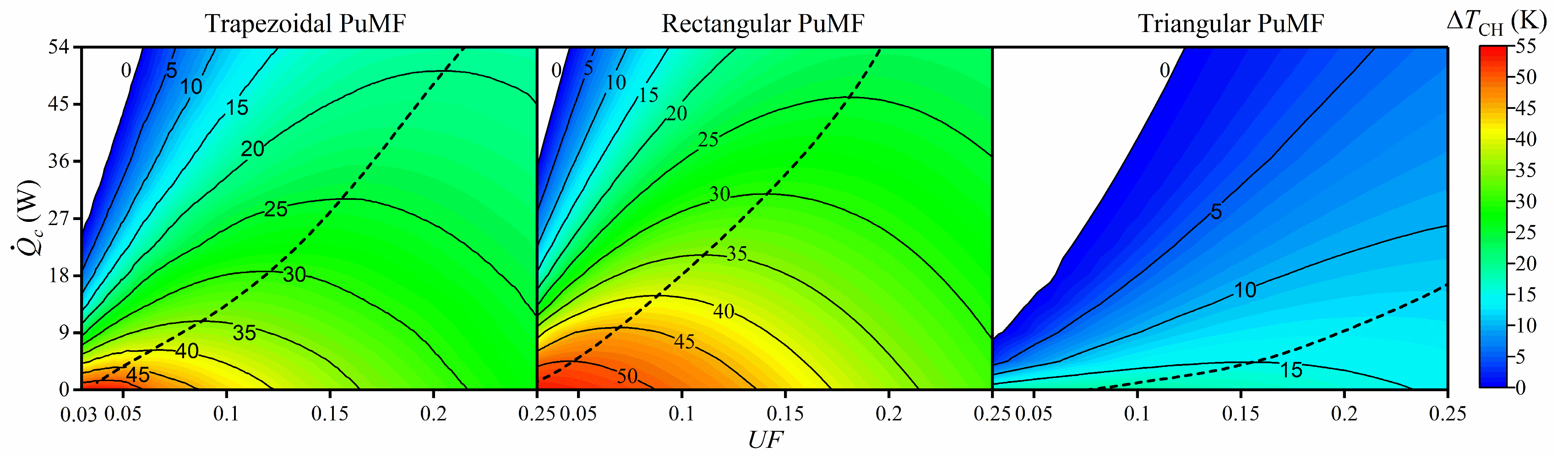
3.3.1. Effect of the Pulsed Magnetic Field Waveform

Figure 8 shows ΔTCH variations, with Q c . for various UFs and magnetic field waveforms. It shows that ΔTCH decreased with an increase in Q c . under all conditions. In addition, the smaller the UF, the more drastic the decrease in ΔTCH. This is because when UF is small, the excessive thermal load at the cold end of the AMR cannot be transferred to the hot end, which leads to a cold-end temperature increase, and then a decrease in ΔTCH. For the three magnetic field waveforms, it was found that when Q c . was equal, ΔTCH was the largest within the rectangular magnetic field and the smallest within the triangular magnetic field. This was because the MCM was magnetized or demagnetized, while simultaneously transferring heat with the HTF in the triangular magnetic field. In this case, the heat transfer quantity between the MCM and HTF was reduced because the MCM was not completely magnetized or demagnetized before heat transfer. Consequently, the hot-end temperature of the AMR decreased, whereas the cold-end temperature increased; therefore, ΔTCH decreased. As for rectangular and trapezoidal magnetic fields, the MCM completed magnetization or demagnetization before the HTF cold or hot blowing; thus, the MCE could be fully utilized. Therefore, the performance of the AMR under the two magnetic fields was higher than that under a triangular magnetic field. Moreover, the performance of the AMR under a rectangular magnetic field was the highest because the magnetization and demagnetization of the MCM were both adiabatic without any loss.
To further explore the performance of the AMR under the three magnetic field waveforms, Q c . and ΔTCH variations with UF were calculated, as shown in Figure 9. Variations of Q c . and ΔTCH with UF were similar under the three magnetic field waveforms; that is, the optimal UF existed. This was because the MCE cannot be fully utilized if the UF is extremely small, and the temperature distribution of the AMR will be disturbed if the UF is extremely large, both of which will reduce Q c . and ΔTCH. Moreover, the performance of the AMR under the rectangular magnetic field was the highest, and that under the triangular magnetic field was the worst. When ΔTCH = 25 K, the maximum Q c . under rectangular and trapezoidal magnetic fields were 45.16 and 30.6 W, respectively. However, the maximum ΔTCH under the triangular magnetic field was only 19.3 K, even if Q c . = 0. The maximum values of ΔTCH under the rectangular and trapezoidal magnetic fields were 54.9 and 54.5 K, respectively, which were 2.84 and 2.82 times that under the triangular magnetic field.

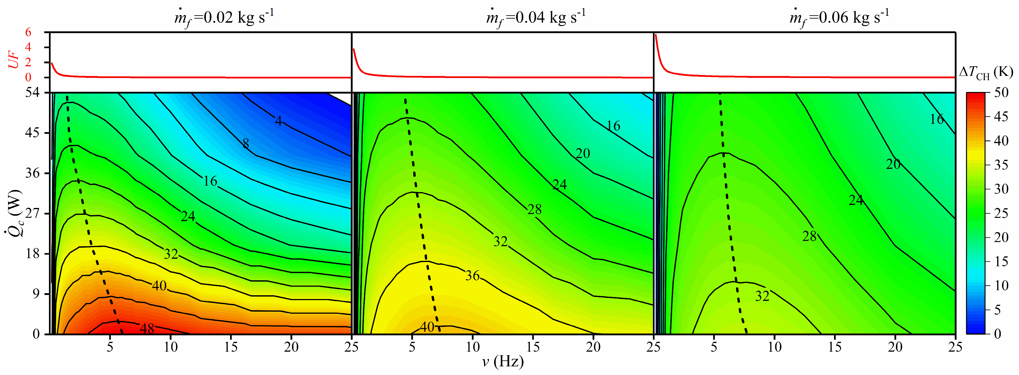
3.3.2. Effect of the Pulsed Magnetic Field Frequency

The existing studies have shown that an increase in the frequency can improve the performance of the AMR. However, whether the higher frequencies are better or not should be explored. The frequency of the pulsed magnetic field can vary over a wide range by adjusting the peak duration, which provides an opportunity to study the effect of high frequency on the performance of the AMR. Figure 10 shows the effects of the magnetic field frequency (ν) on Q c . and ΔTCH at different mass flow rates. It shows that the maximum Q c . was achieved at an optimal frequency when ΔTCH was fixed. The optimum frequency increased with an increasing ΔTCH, as indicated by the dashed lines. Similarly, when Q c . was fixed, the maximum ΔTCH was achieved at an optimal frequency. To better explain the reason, the UFs were calculated, as shown by red lines. The UF was extremely large when the frequency was significantly low, which perturbed the temperature distribution of the AMR and thus decreased the ΔTCH and Q c . . When the frequency was considerably high, the UF was too small to utilize all of the MCEs. In addition, a high frequency implies a considerably short heat-transfer time, which further worsened the transfer of heat. Consequently, Q c . and ΔTCH were reduced. Moreover, both Q c . and ΔTCH highly depend on the frequency when the frequency was extremely low, whereas the dependence was the lowest near the optimal frequency. Therefore, an optimal frequency in the range of 0.93–7.67 Hz was necessary for the AMR to achieve a reasonable cooling performance and stability.
Figure 10 also shows that the contours became sparser under higher mass flow rates, indicating that the dependence of the temperature span on Q c . was weakened. It means that a significant increase in the temperature span can be achieved by reducing a small amount of Q c . at a high mass flow rate.

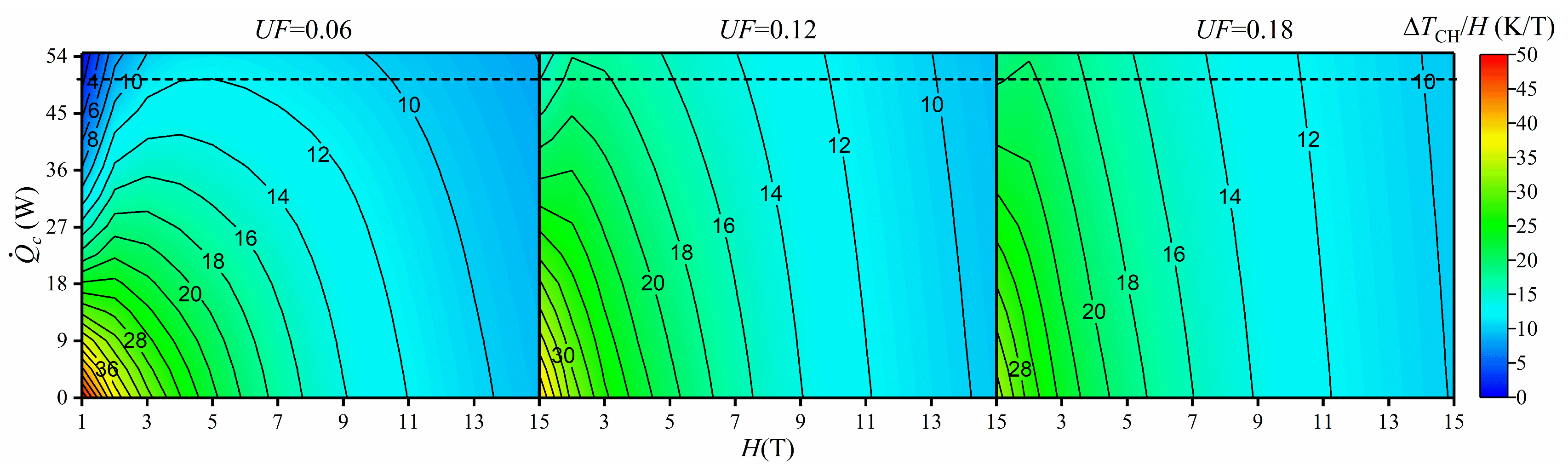
3.3.3. Effect of Pulsed Magnetic Field Intensity

The effect of the magnetic field intensity on the performance of the AMR was investigated under various UFs. In addition to Q c . , we introduced ΔTCH/H as a new evaluation index to characterize the efficiency of the magnetic field. Consequently, a trade-off existed between the performance of the AMR and magnetic field intensity. Figure 11 demonstrates that when ΔTCH/H was constant, a critical magnetic field maximized Q c . , as indicated by the solid lines. Similarly, when Q c . was constant, a critical magnetic field maximized ΔTCH/H, as indicated by the dashed line. The reason was because a trade-off existed between the increased MCE caused by the increased intensity and MCE that the AMR can exploit. Increasing the magnetic field intensity increases the MCE of the MCM, which could significantly improve the cooling performance of the AMR. However, the AMR can only exploit limited MCE because other conditions, such as UF, remain unchanged. Indeed, a simultaneous increase in the magnetic field intensity and UF is more conducive to improving the performance of the AMR.

4. Conclusions

A numerical model based on the energy conservation law was established to investigate the performance of the AMR under the pulsed magnetic field. The model was verified using experiments, with a maximum error of 3.4%. The feasibility of pulsed magnetic refrigeration was demonstrated by simulating the thermodynamic cycle of the AMR. Subsequently, the transient and steady-state performances of the AMR under pulsed and permanent magnetic fields were compared. A stable ΔTCH between the cold and hot ends of AMR could be established in only 0.8 s under the pulsed magnetic field, which was 40 times faster than that under the permanent magnetic field. As for the steady-state performance, the maximum Q c . under a pulsed magnetic field was 2.5 times that of the permanent magnetic field when ΔTCH was 20 K. Moreover, the effects of the pulsed magnetic field waveforms, frequency, and intensity on the performance of AMR were investigated under various UFs.
Consequently, it found that the performance of the AMR was the highest under a rectangular magnetic field, followed by that of the trapezoidal and triangular magnetic fields. The maximum no-load ΔTCH was 54.9 K under the rectangular magnetic field, which was 1.007 and 2.84 times that under the trapezoidal and triangular magnetic fields, respectively. In addition, an optimal frequency in the range of 0.93–7.67 Hz yielded a reasonable cooling performance and stability. Furthermore, a trade-off existed between the performance of the AMR and the intensity of the magnetic field. A critical magnetic field maximizes the performance of AMR and efficiency of the magnetic field, which was found using a newly introduced evaluation index.
However, there are still some challenges of implementing a pulsed magnetic field in new MR applications, such as fast heat transfer of the AMR and acquisition of a pulsed high magnetic field at room temperature. The heat of the magnetic material inside the AMR is gradually brought out by the heat transfer fluid through the AMR, which takes seconds. However, it needs to realize the cyclic heat transfer of the AMR in a few milliseconds to match the high frequency of the pulsed magnetic field. Due to the mechanism of heat convection, the heat transfer speed of the AMR is limited, and AMR fully solid heat transfer could be one of the possible solutions. The generation of pulsed magnetic field requires a cooling system to cool the magnet coil at present, which increases the energy consumption and hinders the implementation of the pulsed magnetic field in new MR applications. Future studies on room-temperature pulsed magnetic fields may solve this problem.

Supplementary Materials

The following supporting information can be downloaded at: https://www.mdpi.com/article/10.3390/en15186804/s1, Figure S1: Magnetocaloric properties of the gadolinium.; Table S1: The related parameter values of gadolinium. References [4,8,16,22,23] are cited in the supplementary materials.

Author Contributions

L.S. completed the writing of the whole manuscript; X.T. completed the data analyses of the simulation and experiment; L.L. provided technical support for the analysis of the pulsed magnetic field; Y.L. completed the analysis of the pulsed magnetic field; Z.L. finished the experiment; and J.X. provided the conception of the whole study. All authors have read and agreed to the published version of the manuscript.

Funding

This work was supported by the Fundamental Research Funds for Central Universities (2021yjsCXCY035).

Institutional Review Board Statement

Not applicable.

Informed Consent Statement

Not applicable.

Data Availability Statement

The data that support the findings of this study are available from the corresponding author upon reasonable request.

Conflicts of Interest

The authors declare no conflict of interest.

References

  1. Krautz, M.; Beyer, L.; Funk, A.; Waske, A.; Weise, B.; Freudenberger, J.; Gottschall, T. Predicting the dominating factors during heat transfer in magnetocaloric composite wires. Mater. Des. 2020, 193, 108832. [Google Scholar] [CrossRef]
  2. Zhang, Y.; Wu, J.; He, J.; Wang, K.; Yu, G. Solutions to obstacles in the commercialization of room-temperature magnetic refrigeration. Renew. Sustain. Energy Rev. 2021, 143, 110933. [Google Scholar] [CrossRef]
  3. Benke, D.; Fries, M.; Gottschall, T.; Ohmer, D.; Taubel, A.; Skokov, K.; Gutfleisch, O. Maximum performance of an active magnetic regenerator. Appl. Phys. Lett. 2021, 119, 203901. [Google Scholar] [CrossRef]
  4. Kitanovski, A.; Tušek, J.; Tomc, U.; Plaznik, U.; Ožbolt, M.; Poredoš, A. Magnetocaloric Energy Conversion; Springer International Publishing: Berlin/Heidelberg, Germany, 2015. [Google Scholar]
  5. Brown, G.V. Magnetic heat pumping near room temperature. J. Appl. Phys. 1976, 47, 3673–3680. [Google Scholar] [CrossRef]
  6. Greco, A.; Aprea, C.; Maiorino, A.; Masselli, C. A review of the state of the art of solid-state caloric cooling processes at room-temperature before 2019. Int. J. Refrig. 2019, 106, 66–88. [Google Scholar] [CrossRef]
  7. Kitanovski, A.; Egolf, P.W. Innovative ideas for future research on magnetocaloric technologies. Int. J. Refrig. 2010, 33, 449–464. [Google Scholar] [CrossRef]
  8. Yang, Z.; Xu, Z.; Wang, J.; Li, Y.; Lin, G.; Chen, J. Thermoeconomic performance optimization of an irreversible Brayton refrigeration cycle using Gd, Gd0.95Dy0.05 or Gd0.95Er0.05 as the working substance. J. Magn. Magn. Mater. 2020, 499, 166189. [Google Scholar]
  9. Zhang, B.; Ding, H.; Wang, S.; Cao, Q.; Liu, M.; Wan, Q.; Xu, Y.; Li, L. Bidirectional repeating long pulse magnet system for magnetic refrigerator. IEEE Trans. Appl. Supercond. 2014, 24, 4900105. [Google Scholar] [CrossRef]
  10. Kihara, T.; Kohama, Y.; Hashimoto, Y.; Katsumoto, S.; Tokunaga, M. Adiabatic measurements of magneto-caloric effects in pulsed high magnetic fields up to 55 T. Rev. Sci. Instrum. 2013, 84, 74901. [Google Scholar] [CrossRef]
  11. Kihara, T.; Katakura, I.; Tokunaga, M.; Matsuo, A.; Kawaguchi, K.; Kondo, A.; Kindo, K.; Ito, W.; Xu, X.; Kainuma, R. Optical imaging and magnetocaloric effect measurements in pulsed high magnetic fields and their application to Ni-Co-Mn-In Heusler alloy. J. Alloys Compd. 2013, 577, S722–S725. [Google Scholar] [CrossRef]
  12. Kihara, T.; Xu, X.; Ito, W.; Kainuma, R.; Tokunaga, M. Direct measurements of inverse magnetocaloric effects in metamagnetic shape-memory alloy NiCoMnIn. Phys. Rev. B 2014, 90, 214409. [Google Scholar] [CrossRef]
  13. Kamantsev, A.P.; Koledov, V.V.; Mashirov, A.V.; Shavrov, V.G.; Yen, N.H.; Thanh, P.T.; Quang, V.M.; Dan, N.H.; Los, A.S.; Gilewski, A.; et al. Measurement of magnetocaloric effect in pulsed magnetic fields with the help of infrared fiber optical temperature sensor. J. Magn. Magn. Mater. 2017, 440, 70–73. [Google Scholar] [CrossRef]
  14. Gottschall, T.; Min MD, K.; Skokov, K.P. Magnetocaloric effect of gadolinium in high magnetic fields. Phys. Rev. 2019, 99, 134429. [Google Scholar] [CrossRef]
  15. Ghorbani Zavareh, M.; Salazar Mejía, C.; Nayak, A.K.; Skourski, Y.; Wosnitza, J.; Felser, C.; Nicklas, M. Direct measurements of the magnetocaloric effect in pulsed magnetic fields: The example of the Heusler alloy Ni50Mn35In15. Appl. Phys. Lett. 2015, 106, 71904. [Google Scholar] [CrossRef]
  16. Chiba, Y.; Smaili, A.; Sari, O. Enhancements of thermal performances of an active magnetic refrigeration device based on nanofluids. Mechanika. 2017, 23, 31–38. [Google Scholar] [CrossRef]
  17. Han, X.; Peng, T.; Ding, H.; Ding, T.; Zhu, Z.; Xia, Z.; Wang, J.; Han, J.; Ouyang, Z.; Wang, Z.; et al. The pulsed high magnetic field facility and scientific research at Wuhan National High Magnetic Field Center. Matter Radiat. Extrem. 2017, 2, 278–286. [Google Scholar] [CrossRef]
  18. Nakashima AT, D.; Dutra, S.L.; Trevizoli, P.V.; Barbosa, J.R. Influence of the flow rate waveform and mass imbalance on the performance of active magnetic regenerators. Part I: Experimental analysis. Int. J. Refrig. 2018, 93, 236–248. [Google Scholar] [CrossRef]
  19. Trevizoli, P.V.; Nakashima, A.T.; Peixer, G.F.; Barbosa, J.R. Performance evaluation of an active magnetic regenerator for cooling applications—Part I: Experimental analysis and thermodynamic performance. Int. J. Refrig. 2016, 72, 192–205. [Google Scholar] [CrossRef]
  20. Qian, S.; Yuan, L.; Yu, J.; Yan, G. Variable load control strategy for room-temperature magnetocaloric cooling applications. Energy 2018, 153, 763–775. [Google Scholar] [CrossRef]
  21. Aprea, C.; Greco, A.; Maiorino, A. The use of the first and of the second order phase magnetic transition alloys for an AMR refrigerator at room temperature: A numerical analysis of the energy performances. Energy Convers. Manag. 2013, 70, 40–55. [Google Scholar] [CrossRef]
  22. Balli, M.; Jandl, S.; Fournier, P.A. Kedous-Lebouc, Advanced materials for magnetic cooling: Fundamentals and practical aspects. Phys. Rev. Appl. 2017, 4, 21305. [Google Scholar] [CrossRef]
  23. Koshkid’Ko, Y.S.; Ćwik, J.; Ivanova, T.I.; Nikitin, S.A.; Miller, M.; Rogacki, K. Magnetocaloric properties of Gd in fields up to 14 T. J. Magn. Magn. Mater. 2017, 433, 234–238. [Google Scholar] [CrossRef]
Figure 1. Typical pulsed and permanent magnetic field waveforms. (a) Pulsed magnetic field; (b) permanent magnetic field.
Energies 15 06804 g001
Figure 2. Schematic diagram of the numerical model.
Energies 15 06804 g002
Figure 3. Experimental apparatus.
Energies 15 06804 g003
Figure 4. Fluid temperatures obtained experimentally and numerically.
Energies 15 06804 g004
Figure 5. Temperature profiles of MCM at the hot and cold ends of the AMR. (H = 1 T, Tc = 288 K, Th = 298 K, UF = 0.06; A: magnetization, B: cold blow, C: demagnetization, and D: hot blow.) (a) Details of the MCM temperature during the first three cycles; (b) temperature profiles of MCM.
Energies 15 06804 g005
Figure 6. Transient variations of the cold-end temperature Ts,c and temperature difference ΔTCH under different UFs (H = 1 T, Q c . = 0 W, Th = Ti = 293 K) (a) Cold-end temperature; (b) yemperature difference.
Energies 15 06804 g006
Figure 7. Steady-state temperature difference Δ TCH and cooling capacity Q c . under different m ˙ f (H = 1 T, Th = Ti = 293 K). (a) Temperature difference; (b) cooling capacity.
Energies 15 06804 g007
Figure 8. Temperature difference ΔTCH variations, with the cooling capacity Q c . under different UFs and magnetic field waveforms (ν = 4.54 Hz, H = 1 T, Th = Ti = 293 K).
Energies 15 06804 g008
Figure 9. Cooling capacity Q c . and temperature difference ΔTCH versus UF under three magnetic field waveforms (ν = 4.54 Hz, H = 1 T, Th = Ti = 293 K, solid line: fixed ΔTCH, dashed line: maximum Q c . under the optimal UF).
Energies 15 06804 g009
Figure 10. Cooling capacity Q c . and temperature difference ΔTCH at different mass flow rates (H = 1 T, Th = Ti = 293 K, solid line: fixed ΔTCH, dashed line: maximum Q c . under the optimal UF).
Energies 15 06804 g010
Figure 11. Cooling capacity Q c . and efficiency of the magnetic field ΔTCH/H versus magnetic field intensity under various UFs (ν = 4.54 Hz, Th = Ti = 293 K, solid line: fixed ΔTCH/H, dashed line: fixed Q c . ).
Energies 15 06804 g011
Table 1. AMR sizes and operating parameters of simulation.
ParameterValue or RangeUnit
AMR length (L)0.1 mm
AMR diameter (D)0.03 mm
Porosity (ε)0.35-
MCM particle diameter (d)0.7 mmmm
Magnetic field intensity (H)1~15T
Magnetic field frequency (ν)0~25Hz
Initial temperature (Ti)293K
Table 2. AMR sizes and operating parameters of experiment.
ParameterValues
AMR sizesL = 0.23 m, D = 0.03 m
ε0.35
ds0.5~0.8 mm
H1.35 T
f0.063 kg/s
ms0.85 kg
Qload50 W
Ti, Tamb293 K
Operating timeτm, τcf, τd, τhf = 1, 2, 1, 2 s
Publisher’s Note: MDPI stays neutral with regard to jurisdictional claims in published maps and institutional affiliations.

