Article

Ensemble Learning Techniques-Based Monitoring Charts for Fault Detection in Photovoltaic Systems

1
Computer, Electrical and Mathematical Sciences and Engineering (CEMSE) Division, King Abdullah University of Science and Technology (KAUST), Thuwal 23955-6900, Saudi Arabia
2
Centre de Développement des Energies Renouvelables, CDER, B.P. 62, Route de l’Observatoire, Algiers 16340, Algeria
3
Laboratoire de Dispositifs de Communication et de Conversion Photovoltaique, Ecole Nationale Polytechnique Alger, Algiers 16200, Algeria
4
Department of Electrical Engineering, University of Sharjah, Sharjah 27272, United Arab Emirates
5
Laboratoire des Technologies de l’Environnement LTE, BP 1523 Al M’naouar ENP Oran, Oran 31000, Algeria
6
Computer Science Department Signal, Image and Speech (SIMPA) Laboratory, University of Science and Technology of Oran-Mohamed Boudiaf (USTO-MB), El Mnaouar, BP 1505, Bir El Djir 31000, Algeria
*
Author to whom correspondence should be addressed.
These authors contributed equally to this work.
Energies 2022, 15(18), 6716; https://doi.org/10.3390/en15186716
Submission received: 19 August 2022 / Revised: 9 September 2022 / Accepted: 11 September 2022 / Published: 14 September 2022

Abstract

:
Over the past few years, there has been a significant increase in the interest in and adoption of solar energy all over the world. However, despite ongoing efforts to protect photovoltaic (PV) plants, they are continuously exposed to numerous anomalies. If not detected accurately and in a timely manner, anomalies in PV plants may degrade the desired performance and result in severe consequences. Hence, developing effective and flexible methods capable of early detection of anomalies in PV plants is essential for enhancing their management. This paper proposes flexible data-driven techniques to accurately detect anomalies in the DC side of the PV plants. Essentially, this approach amalgamates the desirable characteristics of ensemble learning approaches (i.e., the boosting (BS) and bagging (BG)) and the sensitivity of the Double Exponentially Weighted Moving Average (DEWMA) chart. Here, we employ ensemble learning techniques to exploit their capability to enhance the modeling accuracy and the sensitivity of the DEWMA monitoring chart to uncover potential anomalies. In the ensemble models, the values of parameters are selected with the assistance of the Bayesian optimization algorithm. Here, BS and BG are adopted to obtain residuals, which are then monitored by the DEWMA chart. Kernel density estimation is utilized to define the decision thresholds of the proposed ensemble learning-based charts. The proposed monitoring schemes are illustrated via actual measurements from a 9.54 kW PV plant. Results showed the superior detection performance of the BS and BG-based DEWMA charts with non-parametric threshold in uncovering different types of anomalies, including circuit breaker faults, inverter disconnections, and short-circuit faults. In addition, the performance of the proposed schemes is compared to that of BG and BS-based DEWMA and EWMA charts with parametric thresholds.

1. Introduction

Even with the COVID-19-induced economic slowdown, the renewable power sector is continuously experiencing high growth in installed capacity, with more than 260 Gigawatts (GW) in 2021, mostly by solar photovoltaic (PV). This fact led to a total installed capacity of 3064 GW [1]. The highest increase ever is due in large part to political support and cost reductions. In most countries, producing electricity from solar PV and wind is becoming increasingly more cost-effective than generating it from coal and gas power plants [2]. The solar PV market increased in 2021 to a record 175 GWdc, for a total power capacity of 942 GWdc [3]. A recent investigation by the BloombergNEF company shows that the global benchmark levelized cost of electricity (LCOE) [4] for fixed-axis utility-scale PV is $46 per megawatt-hour (MWh) in the first half of 2022, while some of the cheapest PV projects were able to achieve an LCOE of $21/MWh for tracking PV farms in Chile with very competitive returns. In 2022, the solar PV market experienced strong competitiveness between PV module manufacturers with new yields of up to 22.8% [5]. Despite this progress, numerous challenges remain to be solved before solar PV can become a significant source of power generation worldwide, leading to a sustainable energy future [6].
Like all electricity production systems, solar PV systems are often subject to various faults and failures that significantly affect their components, such as PV modules, cables, protection circuits, inverters, etc. [7]. The most general effect of faults is the loss of energy, which is caused by one or more independent anomalies and failures. Some electrical faults cause total shutdowns of PV plants, and other faults such as electric arcs can cause fires, which leads to shortfalls and loss of income. Early detection of such faults is crucial to prevent critical PV system failures and increase their reliability with a high quality of performance. Over the past few years, the Fault Detection and Diagnosis (FDD) of solar PV systems has become a topical research topic for many researchers [8,9]. Generally, anomalies or faults occurring in grid-connected PV systems can be classified primarily according to the side of the fault in the PV installation, either the DC side before the inverter or the AC side at the output of the inverter up to the point of injection [8]. Faults in the DC side of PV systems, which are principally located in the PV array, include; temporary and permanent mismatches, hotspot, degradation, short circuit, open circuit, electrical arc, line–line, and line–ground faults, as well as the DC/DC converter fault inside the PV grid-tie inverter. On the AC side, total blackout and grid abnormalities (unbalanced voltage and lightning) are the types of faults commonly found in PV systems [10]. A statistical study of the power loss evaluation and clustering of faults affecting PV systems installed in different climate zones in the world helps to decrease the number of faults in the new PV installations [11]. The experimental data from PV installed systems show that a better operation and maintenance (O&M) service significantly improves the average performance ratio from 88% to 94%, and as a result, profits and environmental benefits are increased. Indeed, improvements of the PV O&M include the following: (1) increasing efficiency and energy production, (2) extending the lifetime of PV systems (25 to 40 years), (3) decreasing system downtime, (4) reducing the possible risks and ensuring safety and (5) reducing the cost of O&M [12,13].
Continuous and real-time monitoring of PV systems is essential during their working cycle to ensure the rapid detection of faults, reduce downtime, maintain long-term profitability, and exploit their full power. The key point of reliable monitoring and FDD strategy is related to the quality of measurement accuracy of both meteorological and electrical data of the PV system. Without a reliable monitoring system, the PV system is often expected to operate with poor performance for a limited time period before the fault is detected and identified. This fact generally results in a major loss of income [13].
An FDD tool based on the Artificial Neural Network (ANN) algorithm using Laterally Primed Adaptive Resonance Theory (LAPART) was developed in [14] in order to detect module-level faults with minimal error. The results showed that the LAPART algorithm can quickly learn PV performance data (only 4 days of one-minute data) and provide an accurate multi-level FDD tool. Other FDD methods include the k-Nearest Neighbors (kNN) algorithm, which is a non-parametric method used for regression models and fault classification [15]. In [16], four approaches made by EWMA (Exponentially Weighted Moving Average) schemes and kNN-based Shewhart with parametric and non-parametric models were used to detect faults. The results obtained showed a high capability for detecting short-circuit faults, open-circuit faults, and temporary shading, whereas this algorithm does not have the ability to distinguish the partial shading among faults occurring on the DC side of the PV array. A real-time detection and classification technique based on the clustering kNN rule was proposed in [15]. This technique does not require any predefined threshold to classify the faults; the threshold values are unknown and difficult to choose for each PV system due to the strong dependence of the output power on the climatic conditions. In [17], a C4.5 decision tree (DT) approach is proposed to detect and diagnose the faults in a Grid-Connected PV system (GCPV) using a non-parametric model by learning the task. In this work, a semi-empirical model by Sandia National Laboratories (SNL) was used to predict the power produced from the PV array under normal operation conditions (fault-free). Then, the supervised decision tree algorithm was exploited to classify four cases: (1) fault-free, (2) string fault, (3) short-circuit fault, and (4) line-line fault. The results obtained showed a high accuracy of around 99.86% for detection and 99.80% for diagnosis. This supervised learning method requires data from several sets of training examples to build a good classifier that can distinguish between different faults. The authors in [18] used the ANN technique and FL (Fuzzy Logic) system interface to develop a PV FDD algorithm that has been tested to detect ten faults cases, such as a combination of four cases of faulty PV modules and two cases of low and high partial shading. In such a PV FDD algorithm, the voltage and power variations of the studied PV system were used as input for both the ANN technique and the FL system. An unsupervised monitoring approach for detecting anomalies and faults in PV installations using a one-class SVM technique is proposed in [19], where the one-diode model is used under PSIMTM to simulate the normal operation of the PV array, while the one-class SVM technique is applied to calculate residuals between measured and simulation data for FDD. The use of machine learning techniques (MLT) is advantageous in the sense that they have rapid detection response, they allow distinguishing among faults of the same signature and classifying faults with high accuracy, and setting threshold limits is not required. Nevertheless, the FDD accuracy depends proportionally on the trained PV model to estimate the expected energy yield. Moreover, these techniques require more advanced skills for real-time hardware and software implementation, and obtaining a training dataset of all possible faults scenarios could be difficult.
Accurate monitoring of PV plants is necessary to meet the desired specifications regarding power production and safety and help avoid serious incidents. Machine learning techniques have demonstrated themselves as a prominent field of study within a data-driven framework over the last decade by addressing numerous challenging and complex real-world problems [20,21,22,23,24]. Thus, this study aims to design a semi-supervised data-driven detector for anomaly detection in PV plants that do not require labeled data. Unlike supervised methods, semi-supervised anomaly detection methods aim to train the detection model using a normal event dataset only, which make them more attractive for detecting anomalies in PV plants, since it is not always easy to obtain accurately labeled data. Until now, very few research papers have investigated integrating machine learning models and statistical control charts for fault detection in multivariate data. The contribution of this work is threefold as summarized below.
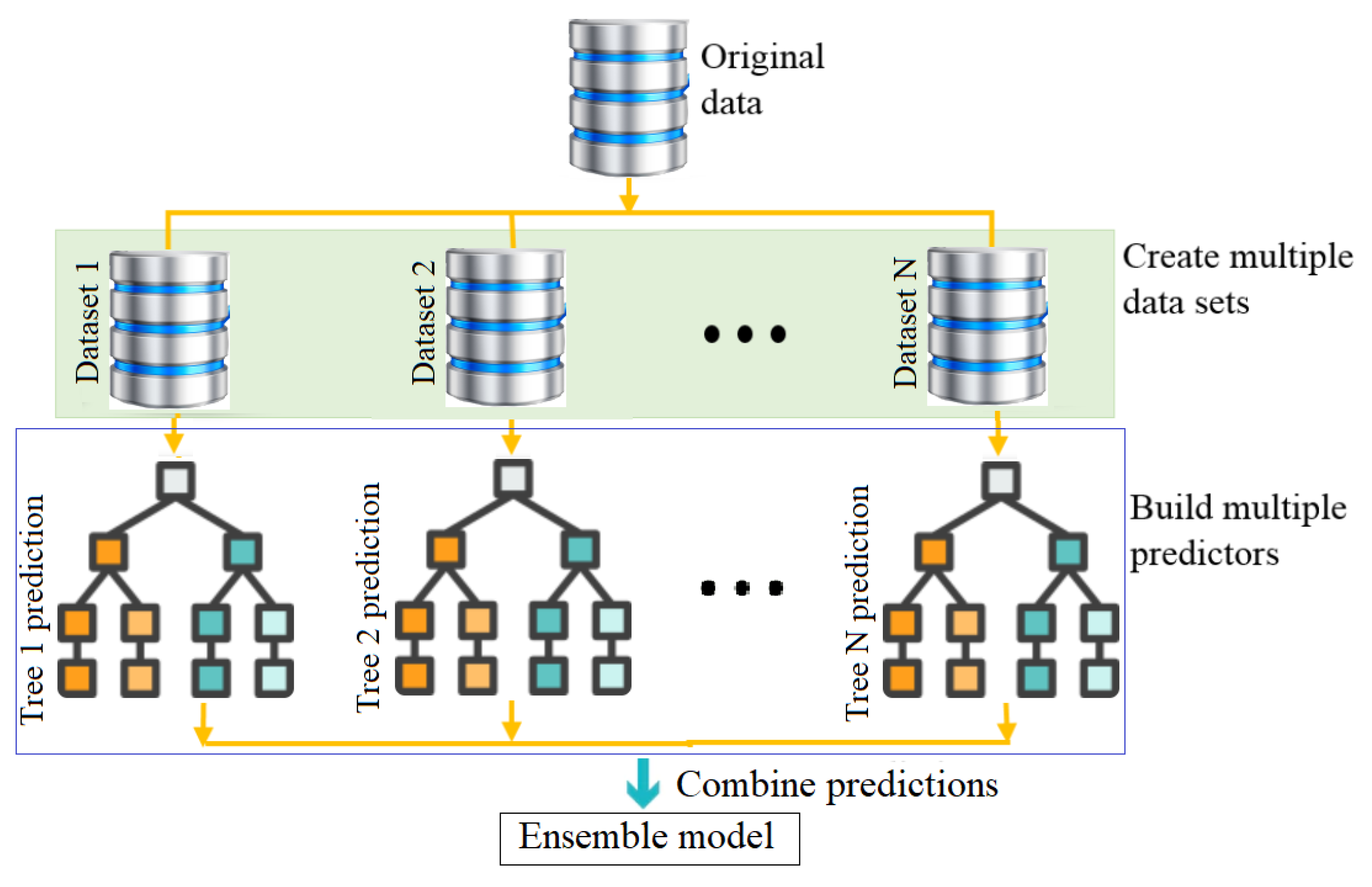
  • This paper aims to develop flexible and efficient semi-supervised machine learning-driven methodologies to improve the operation and performance of PV plants. These semi-supervised approaches only employ normal events data without labeling to train the detection models, making them more attractive for detecting faults in practice. This study presents a semi-supervised monitoring approach for anomaly detection in PV plants by combining the advantages of the ensemble learning models and the Double Exponentially Weighted Moving Average (DEWMA) chart. In the last decade, ensemble learning-driven methods (e.g., boosting and bagging models), which combine several single models, have demonstrated a promising solution compared to traditional machine learning methods. Notably, ensemble models are characterized by their ability to reduce the model’s variance while achieving a low bias, making them appealing to improve prediction quality [25]. Overall, an efficient monitoring strategy relies principally on the accuracy of the adopted modeling method and the sensitivity of the anomaly detection technique. Here, we employed ensemble learning methods to exploit their capability to enhance the modeling precision of the PV monitored system. On the other hand, the key characteristic of the DEWMA scheme resides in its capacity to enclose all of the information from past and actual samples in the detection statistic, which makes it sensitive for uncovering anomalies with small magnitudes. In the proposed approach, ensemble learning models are used for residual generation. Essentially, residuals are close to zero in the absence of anomalies, while residuals diverge from zero in the presence of anomalies. The DEWMA detector is employed to check the generated residuals to uncover possible anomalies in the inspected PV array.
  • Additionally, in this work, Bayesian optimization (BO) has been adopted to optimally tune hyperparameters of the boosted trees (BS) and bagged trees (BG) models. Specifically, the BO is used to find the optimal parameters of the ensemble models based on training data (anomaly-free data). This enables obtaining more accurate prediction models and improves the detection performance.
  • Note that the detection threshold in the DEWMA chart is computed based on the Gaussian assumption of data. Here, to extend further the flexibility of the proposed fault detection method, we employed kernel density estimation (KDE) to compute the detection threshold in a non-parametric way. We assessed the effectiveness of the considered fault detection approaches on real data from a 9.54 kWp photovoltaic system. The detection capacity of the proposed approaches is investigated in the presence of different types of faults. Six statistical scores are computed to judge the fault detection quality. Results revealed the promising performance of the proposed approaches in detecting various types of anomalies in a PV system.
This paper is structured as follows. The studied PV system is briefed in Section 2. Then, the BS and BG models are introduced in Section 3. In Section 4, after presenting the DEWMA scheme, we introduce the proposed approach. The experimental results are provided In Section 5. Lastly, conclusions are offered in Section 6.

2. PV System Description

This section is devoted to presenting briefly the grid-tied PV system used in this study. Indeed, the proposed algorithm for fault detection in this work will be verified using the meteorological and electrical data measurement collected from a 9.54 kWp PV system at the Renewable Energy Development Center (CDER) in Algeria. This PV system contains 90 PV modules with a total power of 9.54 kWdc in operation since 2004; it is composed of three identical single-phase PV sub-systems (Figure 1).
The entire produced PV energy is injected into the low-voltage electrical grid. As shown in Figure 1, each PV sub-system consists of a 3.18 kW sub-array, grid-tie inverter, and electrical cabinets for protection. The sub-array contains two parallel strings of 15 PV modules (PVM) in a series.
Table 1 and Table 2 display, respectively, the main technical specifications of the PV sub-array and the PV inverter.
Here, the STC refers to Standard Test Conditions (irradiance =1000 W/m 2 , cell temperature =25 °C, air mass = 1.5) and MPP denotes Maximum Power Point. G is the received irradiance by the PV module during the flash test, TC is the temperature of the PV cell, and AM is the air mass. VOC is the open circuit voltage, ISC is the short circuit current, VMPP is the voltage at MPP, IMPP is the current at MPP, and PM is the maximum power.
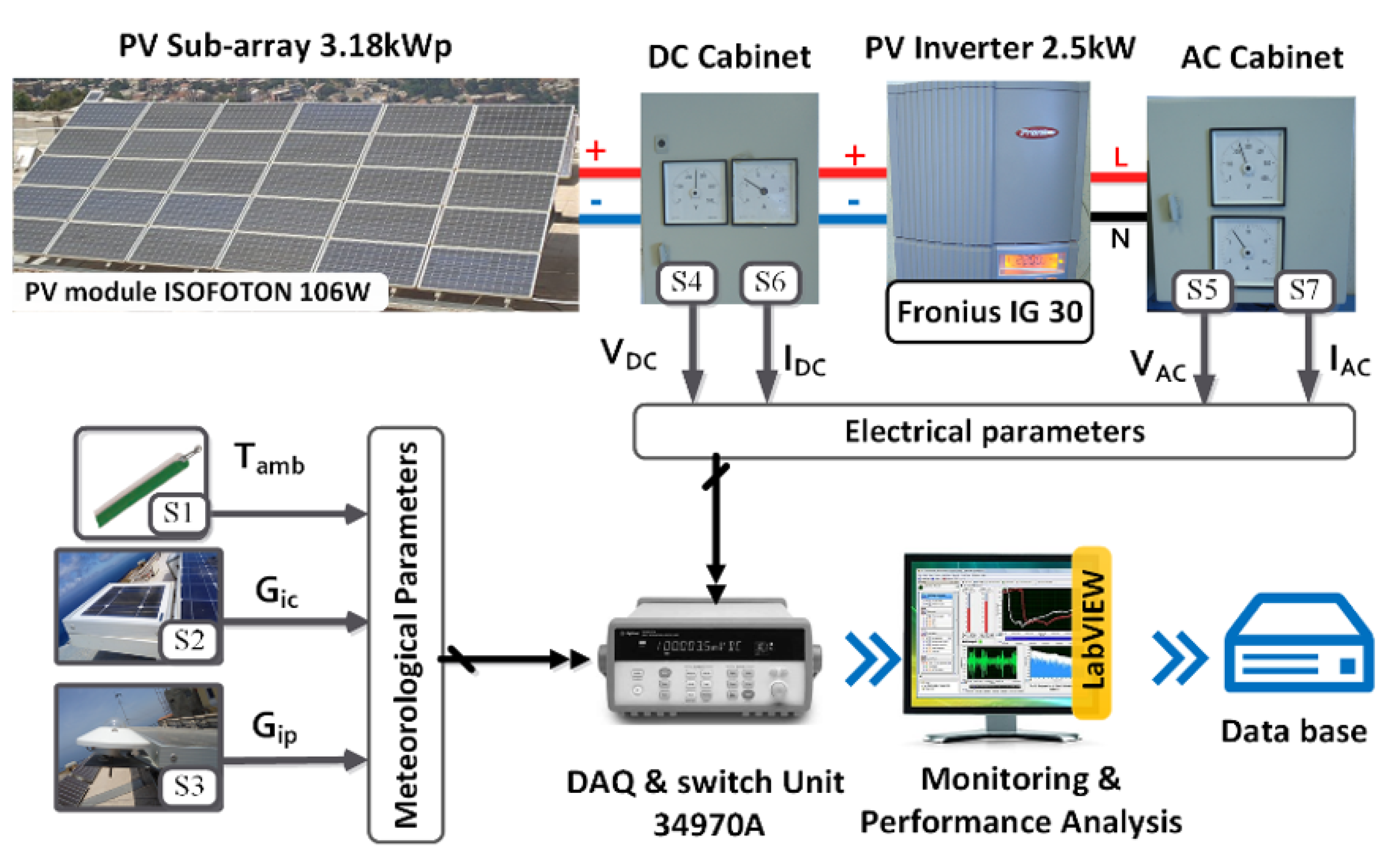
The meteorological and electrical measured data used in this work are recovered by an external monitoring system composed essentially of sensors, data acquisition unit Agilent 34970A, and software under PC (Figure 2).
For the measure of tilted irradiance at 27 °C, a pyranometer and a reference cell are used, and a thermocouple measures the ambient temperature. The DC voltage at the MPP of the PV sub-array is measured by a simple voltage divider circuit, while a voltage transformer measures the AC voltage at the inverter output. A hall-effect sensor was used to measure the current on both the DC and AC sides of the PV inverter. Table 3 reviews the measured parameters with the main sensor information. Agilent 34970A provides the conditioning and the measure of the signal at the sensor’s output. While the monitoring user interface is designed under LabVIEW software, this interface can recover, display, record, and analyze the measured data. According to IEC 61724 standard, the sampling time was chosen at 1 min, which gives 1440 samples per 24 h.

3. Ensemble Learning Methods

This section briefly presents the two considered ensemble learning models: boosting and bagging methods.

3.1. Boosted Trees

The boosting approach, which belongs to ensemble learning models, tries to enhance the prediction accurateness of learning methods by boosting weak learners to strong learners [26,27,28,29,30,31]. This work employs the boosting technique for prediction problems with base learners as regression trees. To introduce the boosting algorithm, regression trees are first briefly described. Let y R and X D R d denote, respectively, the wind power and the input features used in the wind power prediction, where D is the feature space and d is the number of input features.
Regression trees typically are based on the the partition of the feature space D into different and non-overlapping areas, which are known as leaves. The leaves of the regression trees are denoted here by D 1 , , D T , where T denotes the number of leaves. Each leaf D i is associated with a weight w i . For predictions via a given tree, the response is predicted as the weights w i for the input feature X D i . The leaves D i and the weights w i are learned from the training set.
In the process of regression tree training for a given data set { ( X 1 , y 1 ) , , ( X n , y n ) } , the feature space D is recursively partitioned into sub-regions such that the objective function defined by the residual sum of squares (RSS) is minimized until a certain stopping criterion is achieved. The stopping criterion frequently used in the boosting algorithm is a fixed number of leaves. For instance, if only two leaves are considered in a regression tree training, then the feature space D should be split once, and the resulting tree is known as a stump [32]. Indeed, the first step is based on selecting a cut-point s R and an input feature X j from the feature set X = { X 1 , , X d } so that the RSS objective function is minimized. Then, the second step aims at defining the sub-regions D 1 ( j , s ) = { X D | X j s } and D 2 ( j , s ) = { X D | X j > s } .
i : X i D 1 ( j , s ) ( y i y ¯ D 1 ( j , s ) ) 2 + i : X i D 2 ( j , s ) ( y i y ¯ D 2 ( j , s ) ) 2 ,
such that y ¯ D 1 ( j , s ) = i : X i D 1 ( j , s ) y i / n 1 , and  n 1 stands for the number of samples for which the input feature X i D 1 ( j , s ) . y ¯ D 2 ( j , s ) is defined analogously. If a two-leaves tree is trained, then the weight w 1 (resp. w 2 ) corresponding to D 1 ( j , s ) (resp. D 2 ( j , s ) ) is y ¯ D 1 ( j , s ) (resp. y ¯ D 2 ( j , s ) ). The algorithm splits both regression trees D 1 ( j , s ) and D 2 ( j , s ) (same idea of partitioning D ) until the stopping criterion is achieved. Quite often, the weight w i is used as the mean of the response variable in the training data with the corresponding input features D i . More details about regression trees can be found in [33].
To illustrate the boosting algorithm for wind power prediction, let us consider the problem of predicting the wind power y by a function f * ( X ) of input features X so that the risk is minimized,
f * ( X ) = arg min f ( . ) E [ ρ ( y f ( X ) ) ] ,
where ρ ( . ) denotes a loss function ( ρ ( e ) = e 2 is the squared error loss) and arg min stands for the argument of the minimum, that is the function f * ( X ) that minimizes the risk index function over all possible functions under consideration. The boosting algorithm is based on the idea of approximating f * ( X ) by an additive function of the following form
f ( X ) = i = 1 M f i ( X ) ,
where f i ( X ) , i = 1 , , M are regression trees.

3.2. Bagged Regression Trees

Breiman introduced the concept of bootstrap aggregating (bagging) trees by constructing multiple similar but independent predictors, and the final prediction is obtained by averaging the outputs of these predictors [34]. This allows the reduction of the variance error, as pointed out in [35]. In bagging trees/ensembles of decision trees methods, a large number of individual models (trees) are combined with each other (see Figure 3) to improve the quality of prediction of the model. The use of the BGs predictive model is of great importance due to the fact that it allows a reduction of the regression trees’ variance and addressing the over-fitting problem in the regression progress with a single tree.
Figure 3 presents the main idea of a bagging trees predictive model. Such a figure shows that N new training datasets of size n are first created from the original data through the selection of n out of n samples uniformly with replacement from the original training set of data. Then, a training process starts by training individually each tree on the corresponding training new sets. In the present work, the bagging trees models are based on 30 trees. Lastly, the final prediction is obtained by averaging all output predictions. The prediction of the bagging trees model has the following form:
y ^ = 1 N i = 1 N f i ( X ) ,
where the ith tree model f i is trained on the ith bootstrap data.
Theoretically, it is clear that the variance of prediction using n learners can be reduced to 1/n of the original variance (single learner). Thus, the use of a large number of learners is advantageous in the sense that a reduced variance is obtained compared to the prediction with a small numbers of learners. To understand how the bagging process significantly reduces the mean squared error of the prediction, the following regression problem with base regressors b 1 ( x ) , , b n ( x ) is considered. Additional details on BG models can be found in [23].
Algorithm 1 below summarizes the main steps to calculate the bagging trees prediction.
Algorithm 1: Bagging trees approach
Energies 15 06716 i001

4. PV System Modeling and Validation

4.1. Data Analysis

In this study, we used one month of data collected every ten minutes under normal operating conditions to construct the studied machine learning models. The first three weeks are used to train the models, and the last week is testing data to verify the prediction performance of the constructed models. The collected data contain nine variables: solar irradiance, ambient temperature, cell temperature, maximum dynamic DC power, DC current, DC voltage, AC power, AC current, and AC voltage. Figure 4 shows the probability density function of the KDE fit to the nine recorded variables in training data, which indicates that these datasets are non-Gaussian distributed. Table 4 summarizes the descriptive statistics of each variable, which confirm the non-Gaussian distribution of data. It would be challenging for traditional monitoring charts, such as DEWMA and EWMA, that are constructed based on the Gaussian assumption of data.
To quantify the self-similarity in the given time-series data over different delay times, we computed the autocorrelation function (ACF). It is a time-domain measure of the stochastic process memory. Importantly, the ACF for a time-series, x t is expressed as [36],
ρ k = cov x t , x t k var x t var x t k
where cov x t , x t k denotes is the covariance between x t and x t k , and var ( x ) refers to the variance of x. Figure 5 depicts the ACF of the training data. Visually, we clearly observe the presence of an apparent periodicity of 24 h. The time-series periodicity can be identified by measuring the distance between two successive extremum points in the ACF. We suspect this periodicity is caused mainly by the diurnal solar irradiance cycle.
It is important to note that the traditional monitoring charts are designed under the assumption that the data are normally distributed and uncorrelated. However, in many real applications, the normal distribution assumption is violated. In addition, it has been shown in the literature that the performance of the traditional charts is significantly impacted by the presence of autocorrelation [37,38]. Here, we observe from Figure 4 and Figure 5 that the collected data from the inspected PV system are non-Gaussian and correlated. Accordingly, developing advanced monitoring charts based on machine learning is essential.
Figure 6 depicts a Pearson correlation heatmap to highlight correlations between measured variables. We can see from Figure 6 the presence of a strong relationship between the following variables: irradiance, DC current, DC power, AC current, and AC power. The DC current generated by the PV cell, PV module, or PV array is proportional to the tilted irradiance. In the literature, there are many mathematical relationships that explain this high correlation (i.e., more than 0.98) [39,40].
Since the cell temperature is proportional to the irradiance [41,42,43], there is a high positive correlation (i.e., above 0.86) between cell temperature and the following parameters: irradiance, DC current, DC power, AC current, and AC power. Furthermore, the cell temperature is also influenced by variations in the ambient temperature.
The DC voltage of the PV module is the sum of the cell’s voltages in series. It is generally almost stable but decreases when the cell temperature increases [39,40,41], which explains the presence of this negative correlation (i.e., around -0.59). Because the DC voltage is almost stable, the DC power is directly proportional to variations of the DC current.
We observe from Figure 6 the absence of correlation between inverter AC voltage and other variables. Indeed, the PV inverter converts DC energy to AC energy with typical efficiency from 95% to 99% in recent inverters [44,45]. When driving power to the grid, the PV inverter must provide a stable sinusoidal AC waveform that matches grid voltage and frequency according to utility standards to obtain good synchronization.
Figure 6 shows clearly a high correlation between the irradiance, cell temperature, current DC, AC current, power DC and power AC. The data of such a figure show positive and negative correlations as well as low correlation between the DC voltage and the ambient cell temperature, the DC current, AC current, DC power, and AC power. AC voltage does not show a negative weak correlation with other parameters.

4.2. PV Array Modeling Using Ensemble Learning Models

In this study, we used one month of data collected every ten minutes under normal operating conditions to construct the studied machine learning models. The first three weeks are used to train the models, and the last week is testing data to evaluate the prediction accurateness of the constructed models. Here, a fivefold cross-validation procedure is adopted during the training to avoid the over-fitting problem. At first, we used the default parameters for the BT and BST models: 30 learners with a minimum leaf size of 8, and a learning rate of 0.1. We also considered hyperparameter optimization in this study by investigating the performance of the optimized ensemble learning models (OBT and OBST).
Note that one of the most important steps in machine learning-based prediction is hyperparameter tuning or optimization. Optimized ensemble models with tuned hyperparameters are characterized by the highest accuracy and least prediction error based on the training dataset. Broadly speaking, hyperparameters can be computed via the minimization of the loss function (e.g., mean squared error (MSE)) or via the maximization of the prediction accuracy. Of course, the selection of the hyperparameters certainly plays a crucial role in constructing accurate machine learning models, as the efficacy of the model greatly relies on them. In this study, Bayesian optimization (BO) is applied to determine the values of hyperparameters in the two investigated ensemble learning models [23,46]. The main advantage of the BO consists in its capability to select the optimal parameters in an informed manner. More specifically, the BO accounts for the past evaluations when selecting the hyperparameters set to consider next [47], making it less time-consuming compared to both grid search and random search [48,49]. Table 5 lists the calculated values of the hyperparameters of both BT and BST models using the BO procedure.
Figure 7 depicts the actual and the predicted DC power from both the optimized and non-optimized BT and BST models. From Figure 7, it is clear that the ensemble models can catch the trend in the DC power data.
To visually show the prediction accuracy of the four investigated models, Figure 8 contains the boxplots of the prediction errors of each model. It confirms that the optimized models can reach better performance compared to the non-optimized models in predicting DC power. Specifically, we can see that the prediction errors of the optimized BG and BS models fluctuate around zero, indicating that the models can capture the variation and follow the trend in the DC power data. Hence, these boxplots affirm the promising prediction capacity of the two optimized models. Figure 9 illustrates the empirical cumulative distribution function of the prediction errors from the four models; similar conclusions hold true. Figure 9 indicates the superior prediction performance of the OBG model, which is followed by the OBS model.
We also assessed the deviation of the prediction from each model ( y ^ ) and the testing data ( y t ) in quantitative way by computing the three most commonly used statistical metrics: root mean square error (RMSE), mean absolute error (MAE), coefficient of determination ( R 2 ), and mean absolute percentage error (MAPE).
RMSE = 1 n t = 1 n ( y t y ^ t ) 2 ,
MAE = t = 1 n y t y ^ t n ,
R 2 = i = 1 n [ ( y i , y ¯ ) · ( y ^ i y ^ ¯ ) ] 2 i = 1 n ( y i y ¯ ) 2 · i = 1 n ( y ^ i y ^ ¯ ) 2 ,
MAPE = 100 n t = 1 n | y t y ^ t y t | ,
where n denotes the length of the testing data. From Table 6, the results indicate that the optimized models (i.e., OBT and OBST) achieved better prediction accuracy compared to their unoptimized counterparts. This confirms that considering hyperparameter tuning using Bayesian optimization is a very important step to reduce prediction errors and construct more effective models. In addition, results show that the OBST achieved the best performance with an RMSE of 11.36, which is followed by the OBT model with an RMSE of 14.65. Prediction results have been significantly improved by optimizing the prediction models (Table 6).

5. EWMA and DEWMA Monitoring Schemes

This subsection presents the basic idea behind the EWMA and the DEWMA monitoring charts. Unlike Shewhart charts employing only the value of the actual measurement, the EWMA and DEWMA charts, as control charts with memory, are not very sensitive in detecting small and moderate changes. Thus, they are better than Shewhart charts in uncovering changes with small magnitude in the process mean.

5.1. EWMA Monitoring Scheme

Roberts introduced the EWMA chart as a memory chart to bypass the limitations of the Shewhart chart in detecting small changes [50]. In short, the EWMA chart is characterized by its use of information from the past and actual data points, making it sensitive to small changes [51]. Lucas et al. investigated the statistical properties of the EWMA scheme and showed it has similar performance to the CUmulative SUM (CUSUM) scheme in sensing small changes. It is more straightforward to implement and use in practice than the CUSUM chart [52,53,54]. The EWMA statistic is derived as a weighted linear combination of current and past data.
s t = ν x t + ( 1 ν ) s t 1 ; s 0 = μ 0 ,
where ν denotes the smoothing parameter such that 0 < ν 1 , and μ 0 is usually selected to be equal to the mean of fault-free data. Using small values of ν provides less weight to the most recent data points and larger weight to the past observations. In other words, ν regulates the memory depth of the EWMA chart. Crucially, the use of small values of ν enables a more significant influence of the past observations, enabling the EWMA chart to be more capable of sensing small changes [52,55,56]. In practice, ν is usually chosen within the interval [0.15 0.3] for detecting anomalies with small or medium magnitude. We observe that the EWMA chart becomes similar to the Shewhart chart if ν = 1 .
From (10), we obtain the following formula by recursively substituting s t ,
s t = ν j = 0 t 1 ( 1 ν ) t x t j + ( 1 ν ) t s 0 .
We observe from (11) that the weights ν ( 1 ν ) t are decreasing exponentially with time, and the sum of these weights is unity because:
ν j = 0 t 1 ( 1 ν ) t x t j = ν 1 ( 1 ν ) t 1 ( 1 ν ) = 1 ( 1 ν ) t .
The upper and lower detection thresholds of the EWMA scheme are computed using the following equation.
U C L , L C L = μ 0 ± L σ 0 ( ν ( 2 ν ) [ 1 ( 1 ν ) 2 t ] ,
where the factor L represents the width of the decision thresholds. From (13), the asymptotic thresholds are expressed as:
U C L , L C L = μ 0 ± L σ 0 ν ( 2 ν ) .
As it can be noticed, the [ 1 ( 1 ν ) 2 t ] in (13) becomes closer to unity in case of larger t. The EWMA chart signals a potential fault if the EWMA statistic exceeds the decision thresholds. Here, we used the one-sided EWMA chart by using the absolute value of the EWMA charting statistic and only an upper detection threshold. More details on the EWMA chart can be found in [57].

DEWMA Monitoring Approach

The DEWMA chart was introduced in [58,59] to improve the capability of the conventional EWMA approach to sense small changes in the process mean. The basic concept of the DEWMA is founded on the double exponentially weighted moving average, which is a common forecasting technique in time-series analysis. Several authors investigated the performance of the DEWMA in the litterature [60,61,62,63]. It has been shown in [64] that the DEWMA outperformed the EWMA scheme in the detection fault with small and moderate magnitude. The two charts deliver relatively similar results in the case of large and moderate changes [65]. The DEWMA charting statistic, w t is derived as follows,
w 0 = s 0 = μ 0 , w t = ν s t + 1 ν w t 1 , s t = ν x t + 1 ν s t 1 , t = 1 , 2 , , n .
As it can be noticed, in the DEWMA chart, the exponential smoothing is carried out two times, and the w t values are extra smoothed (compared to the s t ). Here, we use DEWMA with equal smoothing constant when computing s t and w t as recommended in [64]. We can compute the variance of w t as,
V a r ( w t ) = ν 4 1 + ( 1 ν ) 2 ( 1 ν ) 2 t ( ( t + 1 ) 2 ( 2 t 2 + 2 t 1 ) ( 1 ν ) 2 + t 2 ( 1 ν ) 4 ) ( 1 ( 1 ν ) 2 ) 3 σ 2 .
The asymptotic variance when t is large is computed as follows,
V a r asymptotic ( w t ) = ν ( 2 2 ν + ν 2 ) ( 2 ν ) 3 σ 2 .
The DEWMA scheme declares an anomaly if the charting statistic w t overpasses the decision thresholds, UCL, and LCL.
U C L , L C L = μ 0 ± k σ ν ( 2 2 ν + ν 2 ) ( 2 ν ) 3 .

5.2. Monitoring PV Systems Using Ensemble Learning Techniques Based DEWMA Chart

As discussed above, there are several motivations for utilizing ensemble learning methods with monitoring charts for fault detection purposes. The main motivation consists in the capacity of ensemble learning methods to model multivariate input–output data, and they outperform their alternative single models in many practical situations. It is known that using ensemble models reduces the prediction error compared to single models. Furthermore, monitoring charts, such as the EWMA and DEWMA, assume that data are uncorrelated. Therefore, there is a consequent need for some ensemble-driven models for generating uncorrelated residuals to enable successful fault detection using monitoring charts. In addition, these integrated ensemble learning techniques-based monitoring charts only employ the data of normal events to train the detection model, making them more attractive for detecting faults in PV systems, since it is not always easy to obtain accurately labeled data.
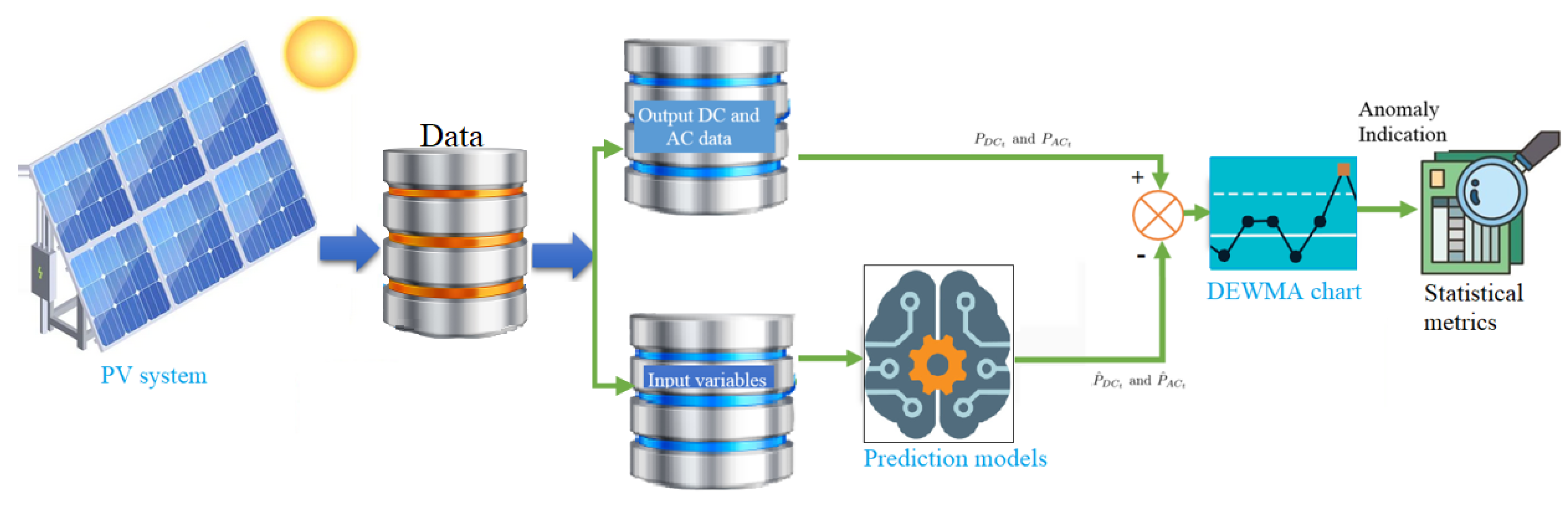
The proposed ensemble learning (BS and BG)-based DEWMA chart to detect anomalies in PV systems is briefly explained in this section and depicted in Figure 10. Specifically, this approach is implemented in two main stages: model construction using training data and fault detection. At first, the ensemble learning models are trained using training data. Here, Bayesian optimization is used to optimally find values of the hyperparameters of the BS and BG models based on training data. In addition, in this step, the detection threshold of the DEWMA and EWMA charts are computed when applied to the residuals obtained from the ensemble learning models. Residuals represent the deviation separating the real output measurements and the predicted values from the ensemble learning model. Under normal operating conditions of the inspected PV systems, the residuals are around zero due to noise measurements and model errors; however, in the case of faulty conditions, the residuals deviate significantly from zero. Here, the ensemble learning models (BS and BG) are trained using fault-free data and then employed for monitoring new data. Then, in the second stage, the constructed models are used for residuals generation, and the DEWMA chart with the previously computed detection threshold is applied to detect potential anomalies in the monitored PV systems.
Note that the decision threshold of the DEWMA and EWMA charts is derived based on the Gaussian distribution of data. However, often in practice, the underlying distribution of data deviates from Gaussianity or is unknown. In such cases, the monitoring results would be unsuitable. To bypass this limitation, in this paper, a non-parametric kernel density estimation (KDE) method was used to set a detection threshold of the DEWMA and EWMA for fault detection. For more details about KDE, refer to [66]. Importantly, it has been shown that the use of KDE to set up the detection threshold does not need to assume that the data follow a Gaussian distribution [67,68], which extends the flexibility of the monitoring charts. Thus, KDE-based detection thresholds are widely employed for process monitoring. A non-parametric detection threshold of the DEWMA chart using KDE is carried out as follows. First, we used KDE to estimate the distribution of the DEWMA statistic based on fault-free data. Given the DEWMA statistic w, the PDF through the KDE is computed as follows.
f ^ ( w ) = 1 n h i = 1 n K w w i h ,
where K ( · ) is the kernel function, and h is the kernel bandwidth parameter and refers to the number of samples. It is mentioned that the Gaussian kernel function is commonly used.
K ( w ) = 1 2 π exp w 2 2 .
Now, the threshold of the distribution-free DEWMA chart is derived as the ( 1 α )-th quantile of the estimated distribution of the DEWMA statistic computed via the KDE. We signal the presence of a potential anomaly if the DEWMA charting statistic exceeds the KDE-based threshold.
The DEWMA with a non-parametric detection threshold is performed as follows:
  • Step 1: Computing the DEWMA charting statistic (Equation (18)) for each observation.
  • Step 2: Estimating the probability density function for given DEWMA measurements via KDE.
  • Step 3: Setting up the detection threshold based on the previously estimated distribution of DEWMA in a non-parametric way as the ( 1 α )-th quantile.
  • Step4: Flagging out a fault if the DEWMA statistic is above the detection threshold.
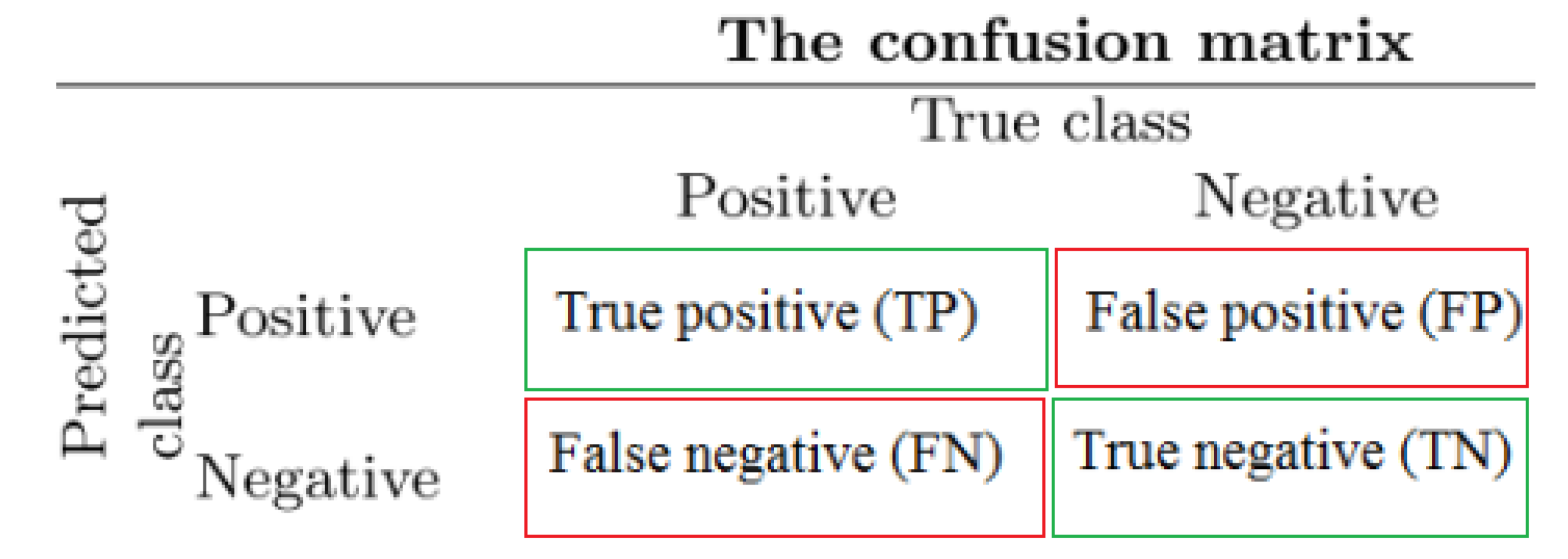
To assess the efficiency of the studied ensemble learning-based monitoring charts, we used six most commonly used performance measures: true positive rate (TPR), false positive rate (FPR), accuracy, recall, F1-score, and area under curve (AUC), and EER (equal error rate) [69]. For a binary detection problem, the number of true positives (TP), false positives (FP), false negatives (FN), and true negatives (TN) is utilized to calculate the performance measures. The 2 × 2 confusion matrix is depicted in Figure 11. The six performance measures are computed as the following.
TPR = TP TP + FN .
FPR = FP TN + FP .
Accuracy = TP + TN TP + TN + FP + FN .
F 1 - score = 2 Precision · Recall Precision + Recall = 2 TP 2 TP + FP + FN .
E E R = F P + F N N F .

6. Results and Discussion

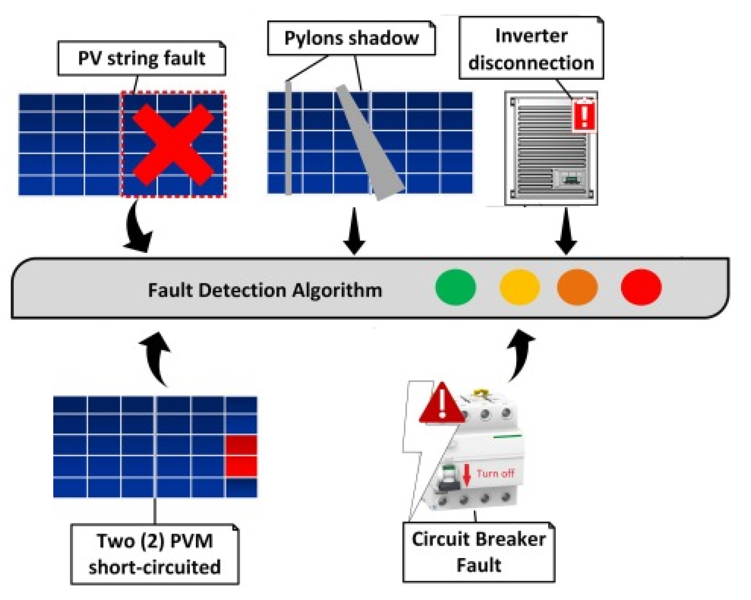
As discussed above, ensemble learning-based monitoring charts enable automatically flagging anomalies in the inspected PV system while avoiding false alarms during normal operating conditions. In this section, the ability of the proposed ensemble learning-based DEWMA schemes to detect anomalies in the DC side of a PV system is assessed. Here, the experimental data were collected from an actual PV system described in Section 2. This study considered five kinds of anomalies: PV string fault (F1), inverter disconnection (F2), circuit breaker faults (F3), partial shading of two pylons (F4), and two PV modules (PVM) short-circuited (F5), as they are represented in Figure 12. For an effective fault detection approach, the TPR, accuracy, F1-score, and AUC values should be close to 1 so that all faulty data are detected. On the other hand, the FPR and EER values should be close to zero to avoid false alarms. For a fair comparison between the competing fault detection methods, in what follows, we used the optimized BG and BS models for each monitoring chart.

6.1. Scenarios with String Faults

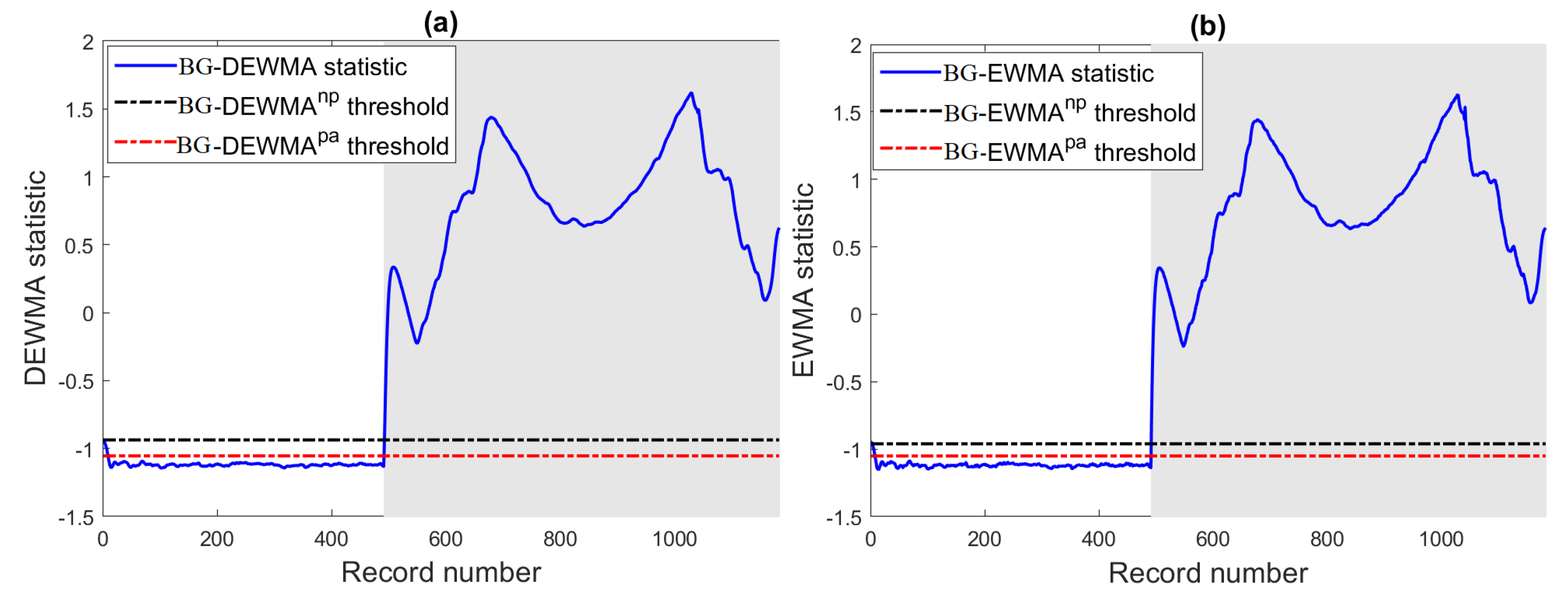
The aim of the first experiment is to study the efficiency of the proposed methods in detecting open-circuit faults in the monitored PV system. Broadly speaking, open-circuit faults could be caused by the deterioration of DC protection or the disconnection between PV modules in series. In this case, a string fault is intentionally generated by switching off the circuit breaker of the PV system. More specifically, we disconnect one string from the PV array. The results of the optimized ensemble models (BG)-based DEWMA and EWMA charts are provided in Figure 13 and show the presence of energy losses in terms of DC power. The results based on BS-based schemes are omitted because they all provide relatively similar results. We observe that the considered monitoring charts with parametric and non-parametric thresholds perform similarly for detecting this severe fault that resulted in a decrease of relatively 50% of the rated power, making it easy to detect by the investigated models.

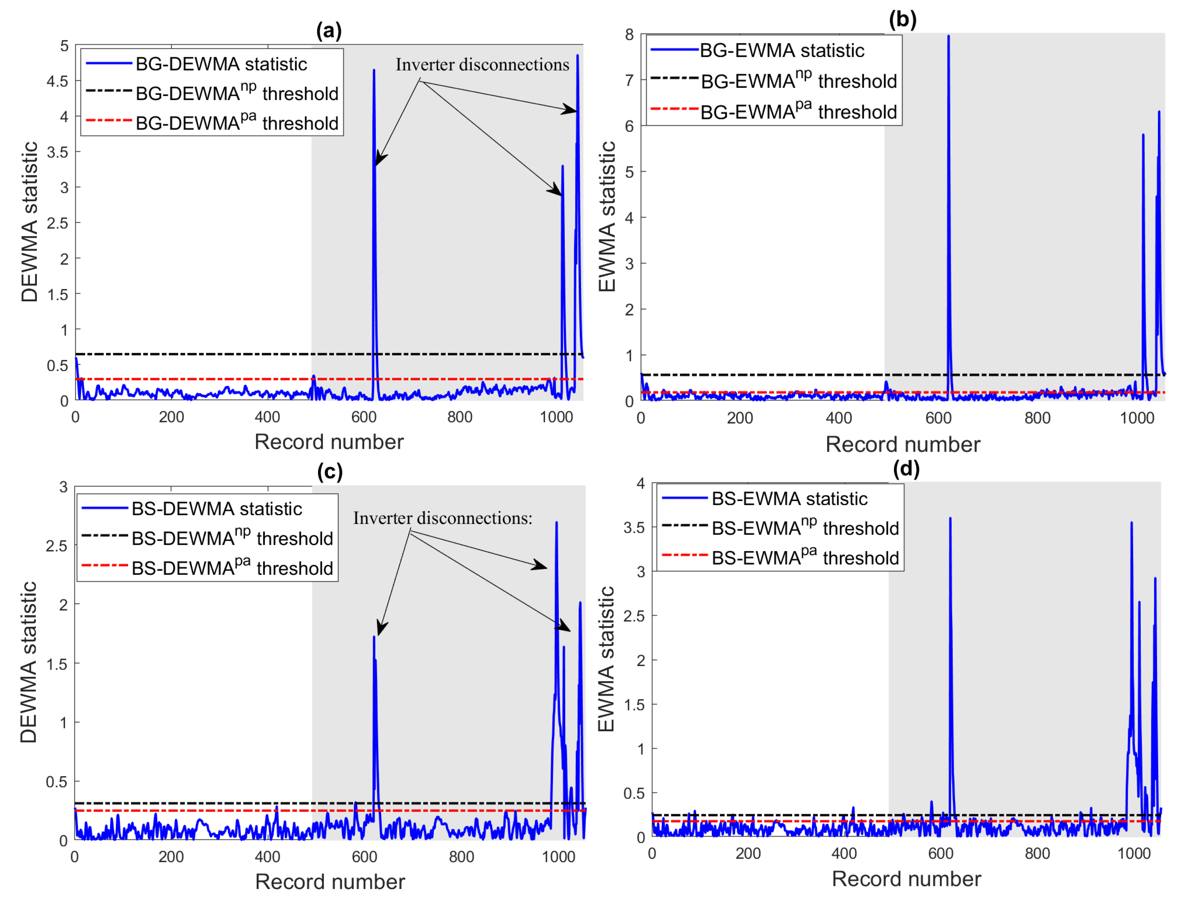
6.2. Scenarios with Inverter Disconnections

In the next experiments, the efficiency of the BG and BS-based DEWMA charts and the competing charts using both parametric and non-parametric thresholds have been investigated in the case of inverter disconnections. Broadly speaking, inverter disconnections are caused if the electrical characteristics exceed the operational limits of the inverter, which are usually given in the datasheet. Note that if inverter disconnections occur, the PV system will shut down until the re-connection of the inverter. In this case study, to verify the detection efficiency of the considered methods, we selected one day of data with inverter disconnection faults. Here, the inverter disconnections are caused by grid instability. More specifically, the voltage and frequency of the grid overpassed the inverter operating limits. Inverter disconnections can be recognized by their very short period and look like spikes, making them easy to discriminate from temporary shading and string faults.
The monitoring results of the investigated ensemble learning-based fault detection charts are depicted in Figure 14. Visually, Figure 14 indicates that these inverter disconnections have been recognized by the considered charts. In addition, we observe that residuals of DC power from the BG and BS models deviate significantly from zero (Figure 14). This means that the constructed models describe well the fault-free data and diverge in the presence of faults. Table 7 lists the detection performance of the considered charts in terms of the five commonly used evaluation scores. As the magnitude of this fault is large, Table 7 clearly indicates that the considered charts easily detect this fault. The results in this table also revealed that the BG and BS-based DEWMA charts with non-parametric thresholds achieved the best performance compared to the other charts. Here, the BS-DEWMA obtained the best detection with an AUC of 0.99, which was followed by the BG-DEWMA chart with an AUC of 0.9881. This could be due to the use of non-parametric thresholds, allowing the DEWMA to be more sensitive than other considered charts. Note that for this fault with a large magnitude, the two types of DEWMA charts (parametric and non-parametric) have slightly similar performance.

6.3. Scenario with Circuit Breaker Faults

The third experiment aimed to assess the ability of the proposed monitoring schemes in detecting circuit breaker fault failures. Crucially, the use of a residual current circuit breaker (RCCB) with a miniature circuit breaker (MCB) is necessary for ensuring the desired performance and protecting PV systems from sudden shock or electrical anomalies. The key role of RCCB is the protection of people from electric shock, and the principal MCB function consists of protecting a PV system against short circuits or overloads. More specifically, the RCCB immediately turns off the power in the presence of a potential electrical fault in the inspected PV system. In this scenario, we generate an RCCB fault within one hour using the collected data. Figure 15 shows the detection performance of the eight investigated ensemble learning-based EWMA and DEWMA charts. We observe that this large fault has been recognized by all the studied charts (Figure 15). We can also see that the BG-DEWMA chart can clearly uncover this fault with reduced false alarms compared to the other charts.
Table 8 presents the performance of the studied BS and BT-based monitoring schemes. From Table 8, it can be clearly seen that BT-based schemes perform slightly better than BS-based schemes. Here, BG-based schemes achieved an AUC of around 0.98, and BS-based schemes obtained an AUC of around 0.97. This means that the considered schemes can efficiently detect this RCCB fault. Results showed that the BG-based EWMA and DEWMA schemes with non-parametric thresholds models reached the highest detection performance in terms of the five evaluation metrics. As the magnitude of the occurred RCCB fault is large, we can see that the BG-based EWMA and DEWMA schemes perform similarly.

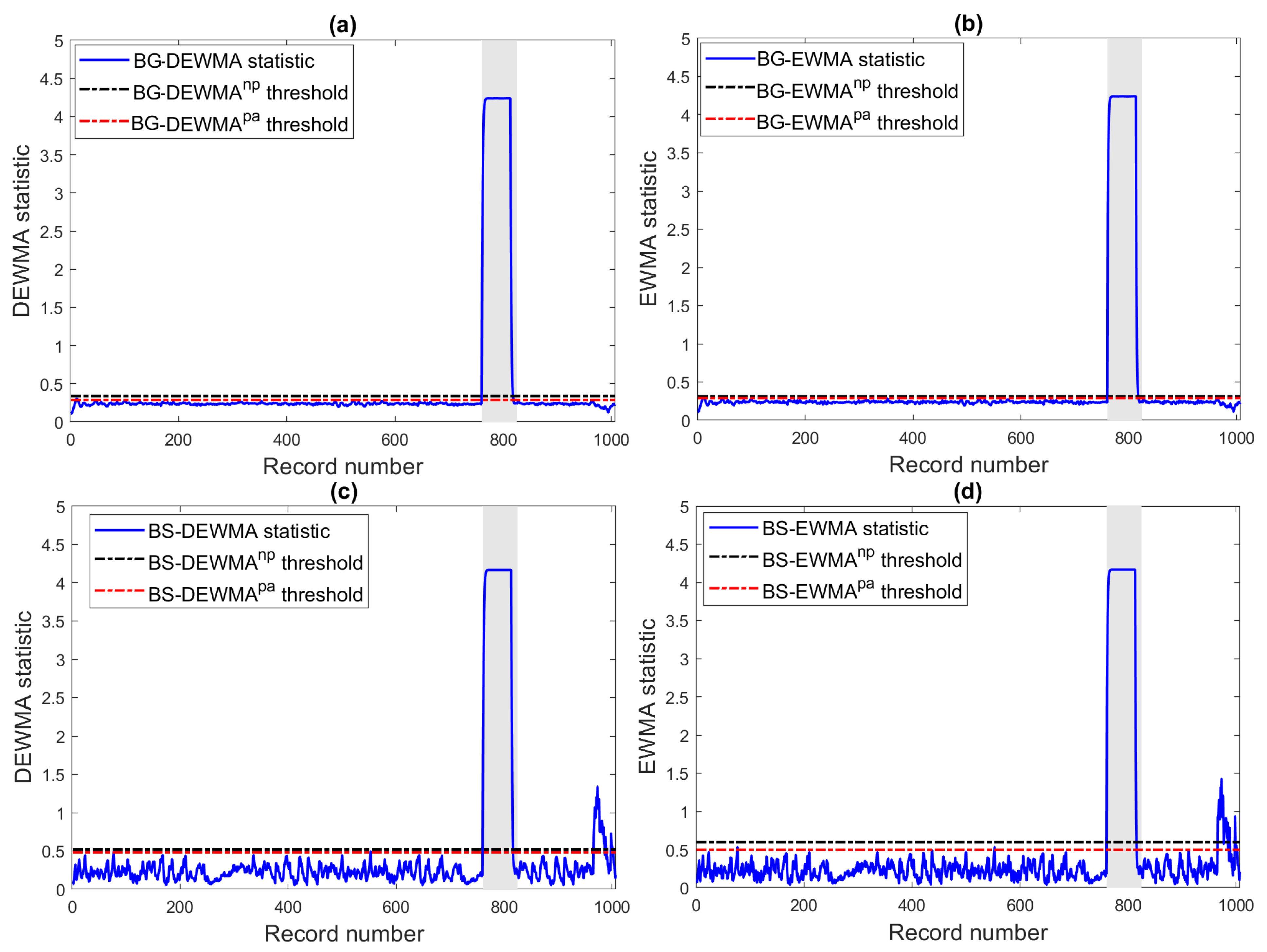
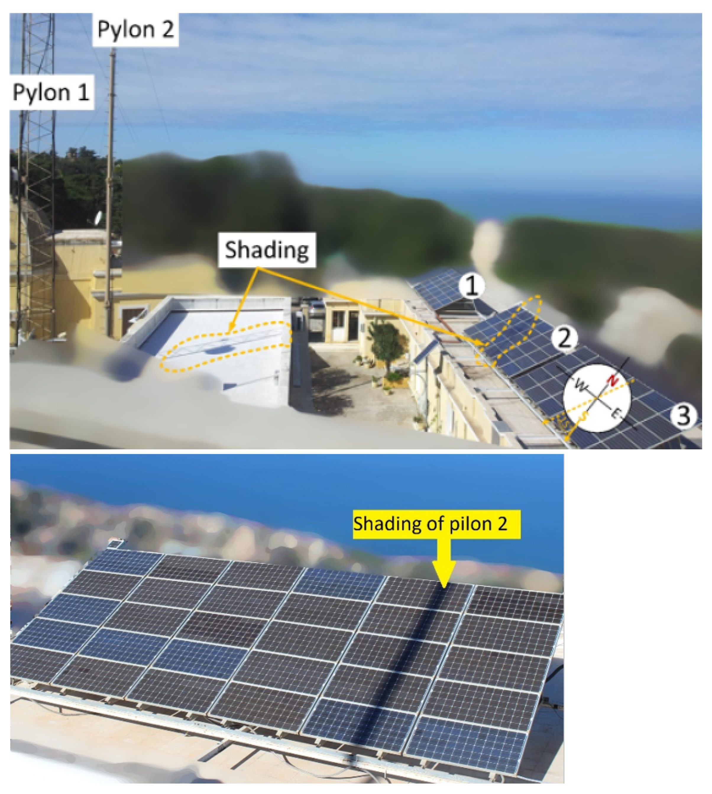
6.4. Scenario with Shaded Modules

Next, the capability of the ensemble learning-based techniques in detecting partial shading is demonstrated. Broadly speaking, different factors can cause shading losses, such as the installation of the PV system close to pylons and trees [8]. Crucially, the production of a PV system exposed to partial shading will decrease from the desired production. Here, the monitored system is exposed to two communication pylons (Figure 16), which can decrease the power output. The data are collected within a period of the day in the presence of partial shading.
The results of the BG and BS-based techniques are depicted in Figure 17. From the plots in Figure 17, we observe that the partial shading of the two pylons resulted in a significant power. It is observed from Figure 17 that the considered charts can sense the presence of this partial shading. So, the proposed ensemble learning-based detection methods effectively flagged out this partial shading. Furthermore, we notice that the BS-based EWMA and DWEMA schemes detect this shading partially, i.e., with some missed detections. On the other hand, all BG-based schemes provide good detection results of this partial shading. Hence, we conclude that the BG model catches most of the variability in the data compared to the BS model, facilitating obtaining more sensitive residuals.
Table 9 shows that the non-parametric DEWMA performed better than the conventional DEWMA and single EWMA schemes with lower FPR and the highest TPR, accuracy, and precision. The non-parametric DEWMA reaches an AUC of 0.984, and the conventional DEWMA and EWMA schemes reached, respectively, AUC values of 0.932 and 0.65. The conventional schemes flag this shading but with some false alarms and missed detection. Such results may indicate the non-parametric DEWMA rather than the conventional DEWMA and EWMA charts for appropriately revealing partial shading in a PV array.
Table 9 lists the detection results of the BG and BS-based techniques in terms of the five evaluation scores. From Table 9, it can be inferred that the BG-based EWMA and DEWMA schemes with non-parametric thresholds outperformed all other methods by providing the best detection performance with a TPR of 0.9805 and very few false alarms (FPR = 0.9869), and an accuracy of 0.9869. This highlights the capacity of these BG-based EWMA and DEWMA schemes in accurately detecting partial shading. Furthermore, it is worth observing that the BG-based schemes with non-parametric thresholds dominate the parametric BG-based schemes’ counterparts. In the parametric schemes, the detection thresholds are determined based on the assumption of the Gaussian distribution of data, which is not often valid. However, in the non-parametric counterparts, the threshold is automatically determined using the KDE approach, making them more effective and flexible. As expected for anomalies with a large magnitude as in this case of partial shading, the DEWMA and the EWMA perform similarly. In contrast, the BS-based monitoring schemes can sense the presence of power loss but with some missed detections. Here, the BS-based DEWMA and EWMA schemes are showing comparable performance with an AUC around 0.89 but with several missed detection (TPR around 0.8).

6.5. Short-Circuit Fault

In this last investigation, we examine the performance of the proposed monitoring schemes in the presence of short-circuit faults. Short-circuit faults if not detected can induce degradation of the PV modules’ performance [70]. In this scenario, the BG and BS-based monitoring schemes are verified in the case of two PV modules short-circuited. The monitoring results of BG and BS-based strategies are presented in Figure 18. Here, the EWMA and DEWMa charts are applied to residual of DC power obtained from the already constructed ensemble learning models (i.e., BG and BT). We observe that the studied monitoring schemes can recognize this short-circuit fault (Figure 18). The BS-based DEWMA and EWMA schemes flag this fault, but with several missed detection. In contrast, BG-based charts detect the fault with minimum false alarms and missed detection.
Table 10 quantitively summarizes the results of BG and BS-based monitoring techniques. From Table 10, the results confirm that the BS-based schemes dominate the BG-based monitoring schemes. In addition, results revealed that the proposed BG-based DEWMA scheme with a non-parametric threshold provides the best results in this case study. It is followed by its parametric counterpart.
In summary, this work shows that merging ensemble learning models to capture describe DC power with the good detection capability of DEWMA enables an efficient detection of anomalies on the DC side of a PV system. The ensemble learning-based fault detection schemes presented in this paper can effectively detect the presence of potential anomalies on the DC sides of the PV system, but they do not identify the types of detected anomaly. Anomaly identification can be performed by the analysis of the DC current and DC voltage. Table 11 lists the influence of the considered anomalies on DC current and DC voltage. Overall, anomaly identification could be conducted by employing semi-supervised anomaly detection methods, such as one-class SVM and isolation forest, to monitor DC current and DC voltage.

7. Conclusions

Accurate fault detection is essential to photovoltaic systems’ efficiency and continuous operation while maintaining the desired performance level. In this work, we developed and studied ensemble learning-based EWMA and DEWMA control charts that are suitable for detecting different anomalies in the AC and DC sides of the PV system. This is mainly motivated by the ensemble learning-driven models’ capability to enhance the performance of machine learning models by merging numerous learners versus single regressors. Specifically, the boosted trees (BST) and bagged trees (BT) models are considered in this study. To enhance the detection performance, we employed Bayesian optimization to find the optimal parameter values of the ensemble learning models based on training data. In addition, kernel density estimation is adopted to non-parametrically determine the detection threshold of the DEWMA chart, which makes it more flexible in dealing with both Gaussian and non-Gaussian data. In order to evaluate the accuracy and performance of the proposed techniques, different electrical faults and environmental anomalies, generally occurring in PV systems, were considered The obtained results showed that the detection and the identification of faults were successfully achieved.
Despite the encouraging obtained results, future research works on PV systems monitoring could be undertaken in several directions:
  • It would be useful to incorporate more data inputs such as open circuit voltage, short circuit current, and fill factor to further enhance the fault detection and diagnosis capabilities of the proposed approach. Moreover, electrical sensors on the AC side of the PV system at the connection point could be added to monitor the energy flow.
  • We also plan to develop deep learning-driven monitoring charts by merging the extended capacity of deep learning models (e.g., long short-term memory (LSTM) and gated recurrent unit (GRU) [71,72]) in automatically extracting important features from multivariate data with statistical monitoring charts such as the generalized likelihood ratio test [73,74] to improve fault detection in PV systems.
  • We plan also to construct parsimonious ensemble learning models by selecting only the important variables for the prediction by the random forest algorithm. Then, the reduced models can be employed for residuals generation to detect faults.
  • Since the DEWMA chart assumes a fixed threshold [75], which may not be suitable to deal with non-stationary (or time-varying) data, adaptive ensemble learning-based DEWMA techniques will be developed in future work by allowing the thresholds of these methods to varying online to account for the changing nature of the data.
  • Data from PV systems are usually tainted with noise measurements, which can degrade the performance of the designed fault detection methods by increasing the number of false alarms and masking pertinent features in data. Future works will improve the robustness of the ensemble learning-based-DEWMA model to noisy measurements by developing a wavelet-based DEWMA detector. Noise effects will be reduced using wavelet-based multiscale denoising; hence, the fault detection performance will significantly be improved.
  • In addition, it will be interesting to investigate the detection capability of the proposed data-driven anomaly detection methodology in other renewable energy systems, such as wind turbine monitoring.

Author Contributions

F.H.: Conceptualization, formal analysis, investigation, methodology, software, supervision, writing—original draft, and writing—review and editing. B.T.: Conceptualization, formal analysis, investigation, methodology, writing—original draft, and writing—review and editing. S.K.: Writing—original draft, and writing—review and editing. A.D.: Formal analysis, methodology, writing—review, and editing. Y.S.: Investigation, conceptualization, formal analysis, methodology, writing—review and editing, funding acquisition, and supervision. A.H.A.: Formal analysis, investigation, review, and editing. All authors have read and agreed to the published version of the manuscript.

Funding

This work was supported by funding from the King Abdullah University of Science and Technology (KAUST), Office of Sponsored Research (OSR), under Award No: OSR-2019-CRG7-3800.

Institutional Review Board Statement

Not applicable.

Informed Consent Statement

Not applicable.

Data Availability Statement

Not applicable.

Conflicts of Interest

The authors declare no conflict of interest.

References

  1. IRENA. Renewable Capacity Statistics 2022; IRENA: Abu Dhabi, United Arab Emirates, 2022. [Google Scholar]
  2. BloombergNEF Cost of New Renewables Temporarily Rises as Inflation Starts to Bite. Available online: https://about.bnef.com/blog/cost-of-new-renewables-temporarily-rises-as-inflation-starts-to-bite/ (accessed on 18 August 2022).
  3. REN21 Renewable Energy Policy, Renewables 2022 Global Status Report; UN Environment Programme: Nairobi, Kenya, 2022.
  4. Caroline, T.; David, M.; Ulrike, J.; Matthias, A.; Ioannis Thomas, T.; Máté, H. Solar Bankability PV Investment Technical Risk Management 2017; Solar Bankability: Brussels, Belgium, 2017. [Google Scholar]
  5. Clean Energy Reviews Most Efficient Solar Panels 2022. 2022. Available online: https://www.cleanenergyreviews.info/blog/most-efficient-solar-panels (accessed on 11 August 2022).
  6. Obeidat, F. A comprehensive review of future photovoltaic systems. Sol. Energy 2018, 163, 545–551. [Google Scholar] [CrossRef]
  7. Richter, M.; Tjengdrawira, C.; Vedde, J.; Green, M.; Frearson, L.; Herteleer, B.; Jahn, U.; Herz, M.; Köntges, M. Technical Assumptions Used in PV Financial Models Review of Current Practices and Recommendations: International Energy Agency Photovoltaic Power Systems Programme: IEA PVPS Task 13, Subtask 1: Report IEA-PVPS T13-08: 2017; International Energy Agency: Paris, France, 2017.
  8. Pillai, D.S.; Rajasekar, N. A comprehensive review on protection challenges and fault diagnosis in PV systems. Renew. Sustain. Energy Rev. 2018, 91, 18–40. [Google Scholar] [CrossRef]
  9. Madeti, S.R.; Singh, S. A comprehensive study on different types of faults and detection techniques for solar photovoltaic system. Sol. Energy 2017, 158, 161–185. [Google Scholar] [CrossRef]
  10. Livera, A.; Theristis, M.; Makrides, G.; Georghiou, G.E. Recent advances in failure diagnosis techniques based on performance data analysis for grid-connected photovoltaic systems. Renew. Energy 2019, 133, 126–143. [Google Scholar] [CrossRef]
  11. Halwachs, M.; Neumaier, L.; Vollert, N.; Maul, L.; Dimitriadis, S.; Voronko, Y.; Eder, G.; Omazic, A.; Mühleisen, W.; Hirschl, C.; et al. Statistical evaluation of PV system performance and failure data among different climate zones. Renew. Energy 2019, 139, 1040–1060. [Google Scholar] [CrossRef]
  12. Walker, H. Best Practices for Operation and Maintenance of Photovoltaic and Energy Storage Systems; Technical Report; National Renewable Energy Lab. (NREL): Golden, CO, USA, 2018.
  13. Lumby, B. Utility-Scale Solar Photovoltaic Power Plants: A Project Developer’s Guide; Technical Report; The World Bank: Washington, DC, USA, 2015. [Google Scholar]
  14. Jones, C.B.; Stein, J.S.; Gonzalez, S.; King, B.H. Photovoltaic system fault detection and diagnostics using Laterally Primed Adaptive Resonance Theory neural network. In Proceedings of the 2015 IEEE 42nd Photovoltaic Specialist Conference (PVSC), New Orleans, LA, USA, 14–19 June 2015; pp. 1–6. [Google Scholar]
  15. Madeti, S.R.; Singh, S. Modeling of PV system based on experimental data for fault detection using kNN method. Sol. Energy 2018, 173, 139–151. [Google Scholar] [CrossRef]
  16. Harrou, F.; Taghezouit, B.; Sun, Y. Improved kNN-based monitoring schemes for detecting faults in PV systems. IEEE J. Photovolt. 2019, 9, 811–821. [Google Scholar] [CrossRef]
  17. Benkercha, R.; Moulahoum, S. Fault detection and diagnosis based on C4. 5 decision tree algorithm for grid connected PV system. Sol. Energy 2018, 173, 610–634. [Google Scholar] [CrossRef]
  18. Dhimish, M.; Holmes, V.; Mehrdadi, B.; Dales, M. Comparing Mamdani Sugeno fuzzy logic and RBF ANN network for PV fault detection. Renew. Energy 2018, 117, 257–274. [Google Scholar] [CrossRef]
  19. Harrou, F.; Dairi, A.; Taghezouit, B.; Sun, Y. An unsupervised monitoring procedure for detecting anomalies in photovoltaic systems using a one-class support vector machine. Sol. Energy 2019, 179, 48–58. [Google Scholar] [CrossRef]
  20. Harrou, F.; Saidi, A.; Sun, Y.; Khadraoui, S. Monitoring of photovoltaic systems using improved kernel-based learning schemes. IEEE J. Photovolt. 2021, 11, 806–818. [Google Scholar] [CrossRef]
  21. Khaldi, B.; Harrou, F.; Benslimane, S.M.; Sun, Y. A data-driven soft sensor for swarm motion speed prediction using ensemble learning methods. IEEE Sens. J. 2021, 21, 19025–19037. [Google Scholar] [CrossRef]
  22. Toubeau, J.F.; Pardoen, L.; Hubert, L.; Marenne, N.; Sprooten, J.; De Grève, Z.; Vallée, F. Machine learning-assisted outage planning for maintenance activities in power systems with renewables. Energy 2022, 238, 121993. [Google Scholar] [CrossRef]
  23. Alkesaiberi, A.; Harrou, F.; Sun, Y. Efficient wind power prediction using machine learning methods: A comparative study. Energies 2022, 15, 2327. [Google Scholar] [CrossRef]
  24. Wang, W.; Harrou, F.; Bouyeddou, B.; Senouci, S.M.; Sun, Y. Cyber-attacks detection in industrial systems using artificial intelligence-driven methods. Int. J. Crit. Infrastruct. Prot. 2022, 38, 100542. [Google Scholar] [CrossRef]
  25. Lee, J.; Wang, W.; Harrou, F.; Sun, Y. Reliable solar irradiance prediction using ensemble learning-based models: A comparative study. Energy Convers. Manag. 2020, 208, 112582. [Google Scholar] [CrossRef]
  26. Freund, Y.; Schapire, R.E. A decision-theoretic generalization of on-line learning and an application to boosting. J. Comput. Syst. Sci. 1997, 55, 119–139. [Google Scholar] [CrossRef]
  27. Bartlett, P.; Freund, Y.; Lee, W.S.; Schapire, R.E. Boosting the margin: A new explanation for the effectiveness of voting methods. Ann. Stat. 1998, 26, 1651–1686. [Google Scholar] [CrossRef]
  28. Schapire, R.E. The boosting approach to machine learning: An overview. In Nonlinear Estimation and Classification; Springer: Berlin/Heidelberg, Germany, 2003; pp. 149–171. [Google Scholar]
  29. Bühlmann, P.; Hothorn, T. Boosting algorithms: Regularization, prediction and model fitting. Stat. Sci. 2007, 22, 477–505. [Google Scholar]
  30. Chen, T.; Guestrin, C. Xgboost: A scalable tree boosting system. In Proceedings of the 22nd acm Sigkdd International Conference on Knowledge Discovery and Data Mining, San Francisco, CA, USA, 13–17 August 2016; pp. 785–794. [Google Scholar]
  31. Bibi, N.; Shah, I.; Alsubie, A.; Ali, S.; Lone, S.A. Electricity Spot Prices Forecasting Based on Ensemble Learning. IEEE Access 2021, 9, 150984–150992. [Google Scholar] [CrossRef]
  32. Friedman, J.; Hastie, T.; Tibshirani, R. Additive logistic regression: A statistical view of boosting (with discussion and a rejoinder by the authors). Ann. Stat. 2000, 28, 337–407. [Google Scholar] [CrossRef]
  33. Breiman, L.; Friedman, J.; Olshen, R.; Stone, C. Classification and Regression Trees; Chapman & Hall: London, UK, 1984. [Google Scholar]
  34. Breiman, L. Bagging predictors. Mach. Learn. 1996, 24, 123–140. [Google Scholar] [CrossRef]
  35. Sutton, C.D. Classification and regression trees, bagging, and boosting. Handb. Stat. 2005, 24, 303–329. [Google Scholar]
  36. Box, G.E.; Jenkins, G.M.; Reinsel, G.C.; Ljung, G.M. Time Series Analysis: Forecasting and Control; John Wiley & Sons: Hoboken, NJ, USA, 2015. [Google Scholar]
  37. Alwan, L.C. Effects of autocorrelation on control chart performance. Commun. Stat.-Theory Methods 1992, 21, 1025–1049. [Google Scholar] [CrossRef]
  38. Leoni, R.C.; Costa, A.F.B.; Machado, M.A.G. The effect of the autocorrelation on the performance of the T2 chart. Eur. J. Oper. Res. 2015, 247, 155–165. [Google Scholar] [CrossRef]
  39. Stein, J.S.; Klise, G.T. Models Used to Assess the Performance of Photovoltaic Systems; Technical Report; Sandia National Laboratories (SNL): Albuquerque, NM, USA; Livermore, CA, USA, 2009.
  40. King, D.L.; Kratochvil, J.A.; Boyson, W.E. Photovoltaic Array Performance Model. 2004. Available online: http://www.mauisolarsoftware.com/MSESC/xPerfModel2003.pdf (accessed on 18 August 2022).
  41. Rawat, R.; Kaushik, S.; Lamba, R. A review on modeling, design methodology and size optimization of photovoltaic based water pumping, standalone and grid connected system. Renew. Sustain. Energy Rev. 2016, 57, 1506–1519. [Google Scholar] [CrossRef]
  42. Mora Segado, P.; Carretero, J.; Sidrach-de Cardona, M. Models to predict the operating temperature of different photovoltaic modules in outdoor conditions. Prog. Photovolt. Res. Appl. 2015, 23, 1267–1282. [Google Scholar] [CrossRef]
  43. Nguyen, D.P.N.; Neyts, K.; Lauwaert, J. Proposed Models to Improve Predicting the Operating Temperature of Different Photovoltaic Module Technologies under Various Climatic Conditions. Appl. Sci. 2021, 11, 7064. [Google Scholar] [CrossRef]
  44. Boyson, W.E.; Galbraith, G.M.; King, D.L.; Gonzalez, S. Performance Model for Grid-Connected Photovoltaic Inverters; Technical Report; Sandia National Laboratories (SNL): Albuquerque, NM, USA; Livermore, CA, USA, 2007.
  45. Driesse, A.; Jain, P.; Harrison, S. Beyond the curves: Modeling the electrical efficiency of photovoltaic inverters. In Proceedings of the 2008 33rd IEEE Photovoltaic Specialists Conference, San Diego, CA, USA, 11–16 May 2008; pp. 1–6. [Google Scholar]
  46. Protopapadakis, E.; Voulodimos, A.; Doulamis, N. An investigation on multi-objective optimization of feedforward neural network topology. In Proceedings of the 2017 8th International Conference on Information, Intelligence, Systems & Applications (IISA), Larnaca, Cyprus, 27–30 August 2017; pp. 1–6. [Google Scholar]
  47. Shahriari, B.; Swersky, K.; Wang, Z.; Adams, R.P.; De Freitas, N. Taking the human out of the loop: A review of Bayesian optimization. Proc. IEEE 2015, 104, 148–175. [Google Scholar] [CrossRef]
  48. Snoek, J.; Larochelle, H.; Adams, R.P. Practical bayesian optimization of machine learning algorithms. Adv. Neural Inf. Process. Syst. 2012, 25. Available online: https://proceedings.neurips.cc/paper/2012/hash/05311655a15b75fab86956663e1819cd-Abstract.html (accessed on 18 August 2022).
  49. Nguyen, V.H.; Le, T.T.; Truong, H.S.; Le, M.V.; Ngo, V.L.; Nguyen, A.T.; Nguyen, H.Q. Applying Bayesian Optimization for Machine Learning Models in Predicting the Surface Roughness in Single-Point Diamond Turning Polycarbonate. Math. Probl. Eng. 2021, 2021, 6815802. [Google Scholar] [CrossRef]
  50. Roberts, S. Control chart tests based on geometric moving averages. Technometrics 2000, 42, 97–101. [Google Scholar] [CrossRef]
  51. Hunter, J.S. The exponentially weighted moving average. J. Qual. Technol. 1986, 18, 203–210. [Google Scholar] [CrossRef]
  52. Montgomery, D.C. Introduction to Statistical Quality Control; John Wiley & Sons: Hoboken, NJ, USA, 2020. [Google Scholar]
  53. Khaldi, B.; Harrou, F.; Cherif, F.; Sun, Y. Monitoring a robot swarm using a data-driven fault detection approach. Robot. Auton. Syst. 2017, 97, 193–203. [Google Scholar] [CrossRef]
  54. Harrou, F.; Nounou, M.; Nounou, H. A statistical fault detection strategy using PCA based EWMA control schemes. In Proceedings of the 2013 9th Asian Control Conference (ASCC), Istanbul, Turkey, 23–26 June 2013; pp. 1–4. [Google Scholar]
  55. Zeroual, A.; Harrou, F.; Sun, Y.; Messai, N. Integrating model-based observer and Kullback–Leibler metric for estimating and detecting road traffic congestion. IEEE Sens. J. 2018, 18, 8605–8616. [Google Scholar] [CrossRef]
  56. Harrou, F.; Sun, Y.; Madakyaru, M.; Bouyedou, B. An improved multivariate chart using partial least squares with continuous ranked probability score. IEEE Sens. J. 2018, 18, 6715–6726. [Google Scholar] [CrossRef]
  57. Lucas, J.; Saccucci, M. Exponentially weighted moving average control schemes: Properties and enhancements. Technometrics 1990, 32, 1–12. [Google Scholar] [CrossRef]
  58. Shamma, S.E.; Shamma, A.K. Development and evaluation of control charts using double exponentially weighted moving averages. Int. J. Qual. Reliab. Manag. 1992, 9. [Google Scholar] [CrossRef]
  59. Shamma, S.E.; Amin, R.W.; Shamma, A.K. A double exponentially weigiited moving average control procedure with variable sampling intervals. Commun. Stat.-Simul. Comput. 1991, 20, 511–528. [Google Scholar] [CrossRef]
  60. Mahmoud, M.A.; Woodall, W.H. An evaluation of the double exponentially weighted moving average control chart. Commun. Stat. Comput. 2010, 39, 933–949. [Google Scholar] [CrossRef]
  61. Khoo, M.B.; Teh, S.; Wu, Z. Monitoring process mean and variability with one double EWMA chart. Commun. Stat. Methods 2010, 39, 3678–3694. [Google Scholar] [CrossRef]
  62. Adeoti, O.A.; Malela-Majika, J.C. Double exponentially weighted moving average control chart with supplementary runs-rules. Qual. Technol. Quant. Manag. 2020, 17, 149–172. [Google Scholar] [CrossRef]
  63. Raza, M.A.; Nawaz, T.; Aslam, M.; Bhatti, S.H.; Sherwani, R.A.K. A new nonparametric double exponentially weighted moving average control chart. Qual. Reliab. Eng. Int. 2020, 36, 68–87. [Google Scholar] [CrossRef]
  64. Zhang, L.; Chen, G. An extended EWMA mean chart. Qual. Technol. Quant. Manag. 2005, 2, 39–52. [Google Scholar] [CrossRef]
  65. Taghezouit, B.; Harrou, F.; Sun, Y.; Arab, A.H.; Larbes, C. A simple and effective detection strategy using double exponential scheme for photovoltaic systems monitoring. Sol. Energy 2021, 214, 337–354. [Google Scholar] [CrossRef]
  66. Rosenblatt, M. Curve estimates. Ann. Math. Stat. 1971, 42, 1815–1842. [Google Scholar] [CrossRef]
  67. Chen, Q.; Wynne, R.; Goulding, P.; Sandoz, D. The application of principal component analysis and kernel density estimation to enhance process monitoring. Control Eng. Pract. 2000, 8, 531–543. [Google Scholar] [CrossRef]
  68. Taghezouit, B.; Harrou, F.; Sun, Y.; Arab, A.H.; Larbes, C. Multivariate statistical monitoring of photovoltaic plant operation. Energy Convers. Manag. 2020, 205, 112317. [Google Scholar] [CrossRef]
  69. Harrou, F.; Khaldi, B.; Sun, Y.; Cherif, F. An efficient statistical strategy to monitor a robot swarm. IEEE Sens. J. 2019, 20, 2214–2223. [Google Scholar] [CrossRef]
  70. Pei, T.; Hao, X. A Fault Detection Method for Photovoltaic Systems Based on Voltage and Current Observation and Evaluation. Energies 2019, 12, 1712. [Google Scholar] [CrossRef]
  71. Harrou, F.; Kadri, F.; Sun, Y. Forecasting of photovoltaic solar power production using LSTM approach. Adv. Stat. Model. Forecast. Fault Detect. Renew. Energy Syst. 2020, 3. Available online: https://library.oapen.org/bitstream/handle/20.500.12657/43847/external_content.pdf?sequence=1#page=17 (accessed on 18 August 2022).
  72. Harrou, F.; Sun, Y.; Hering, A.S.; Madakyaru, M. Statistical Process Monitoring Using Advanced Data-Driven and Deep Learning Approaches: Theory and Practical Applications; Elsevier: Amsterdam, The Netherlands, 2020. [Google Scholar]
  73. Harrou, F.; Zeroual, A.; Sun, Y. Traffic congestion detection based on hybrid observer and GLR test. In Proceedings of the 2018 Annual American Control Conference (ACC), Milwaukee, WI, USA, 27–29 June 2018; pp. 604–609. [Google Scholar]
  74. Madakyaru, M.; Harrou, F.; Sun, Y. Improved anomaly detection using multi-scale PLS and generalized likelihood ratio test. In Proceedings of the 2016 IEEE Symposium Series on Computational Intelligence (SSCI), Athens, Greece, 6–9 December 2016; pp. 1–6. [Google Scholar]
  75. Knoth, S.; Saleh, N.A.; Mahmoud, M.A.; Woodall, W.H.; Tercero-Gómez, V.G. A critique of a variety of “memory-based” process monitoring methods. J. Qual. Technol. 2022, 1–27. [Google Scholar] [CrossRef]
Figure 1. Main electrical specifications of the PV module and sub-array at STC.
Energies 15 06716 g001
Figure 2. Synoptic diagram of the PV monitoring system.
Energies 15 06716 g002
Figure 3. Schematic drawing of the concept of the BG model.
Energies 15 06716 g003
Figure 4. Distribution of the investigated time-series data.
Energies 15 06716 g004
Figure 5. Sample ACF of the training data.
Energies 15 06716 g005
Figure 6. A Pearson correlation heatmap of data.
Energies 15 06716 g006
Figure 7. Power prediction using BG, BS, OBG, and OBS models based on training data.
Energies 15 06716 g007
Figure 8. Boxplot of residual errors of bagged tree, boosted tree, optimized BG, and optimized BS models.
Energies 15 06716 g008
Figure 9. Empirical CDF of the prediction errors for the invstigated models.
Energies 15 06716 g009
Figure 10. The framework of the proposed ensemble learning-driven fault detection technique.
Energies 15 06716 g010
Figure 11. Performance indices used in fault detection.
Energies 15 06716 g011
Figure 12. Considered anomalies in this study.
Energies 15 06716 g012
Figure 13. Results of the BG-based schemes in monitoring a string fault: (a) BG-DEWMA scheme, and (b) BG-DEWMA scheme.
Energies 15 06716 g013
Figure 14. Results of the BG and BS-based schemes in monitoring inverter disconnections: (a) BG-DEWMA, (b) BG-EWMA, (c) BS-DEWMA, and (d) BS-EWMA schemes.
Energies 15 06716 g014
Figure 15. Results of the BG and BS-based schemes in monitoring a circuit breaker fault: (a) BG-DEWMA, (b) BG-EWMA, (c) BS-DEWMA, and (d) BS-EWMA schemes.
Energies 15 06716 g015
Figure 16. (Top) PV array with shaded modules due to two communication pylons installed in front of this PV array. (Bottom) Shading of pylon 2 on PV sub-array 2.
Energies 15 06716 g016
Figure 17. Results of the BG and BS-based schemes in monitoring partial shading: (a) BG-DEWMA, (b) BG-EWMA, (c) BS-DEWMA, and (d) BS-EWMA schemes.
Energies 15 06716 g017
Figure 18. Results of the BG-based schemes in the presence of two short-circuited modules: (a) BG-DEWMA, (b) BG-EWMA, (c) BS-DEWMA, and (d) BS-EWMA schemes.
Energies 15 06716 g018
Table 1. Main electrical specifications of the PV module and PV sub-array at STC.
Parameters V OC (V) I SC (A) V MPP (V) I MPP (A) P M (W)
PV Module21.66.5417.46.1106
PV sub-array32413.0826112.23180
Table 2. Main specifications of the PV inverters Fronuis IG 30 under nominal operating conditions.
ParametersNominal AC
Power (W)
DC Voltage Range (V)AC Voltage Range (V)Inverter Efficiency (%)Frequency Range (Hz)
Value2500150–400195–25392.7–94.349.8–50.2
Table 3. Measured parameters of the PV inverters Fronuis IG 30 under nominal operating conditions.
Measured ParametersSensor N°SymbolSensor Type & ReferenceAccuracy
Ambient Temperature (°C)S1TambThermocouple K0.5 °C
Tilted Global Irradiance for 27° (W/m2)S2GicIsofoton PV Reference Cell±5%
S3GipCM 11 Pyranometer±2%
PV array DC Voltage (V)S4VDCVoltage Divider±0.9%
Grid AC Voltage (V)S5VACVoltage Transformer1.5%
PV array DC Current (A)S6IDCHall Effect Sensor±0.5%
Inverter AC Current (A)S7IACF.W. BELL CLSM-50S
Table 4. Descriptive statistics of the training data.
MinMaxSTDQ 0.25Q 0.5Q 0.75SkewnessKurtosis
Ambient Temp14.5137.224.6122.2626.0429.14−0.222.36
Cell Temp16.1264.4711.2133.4344.0752.49−0.251.98
Irradiance42.671085.10312.30277.07614.26862.42−0.211.65
DC voltage205.56263.199.24227.58233.76240.110.012.78
DC current0.5011.783.223.226.578.96−0.221.76
AC voltage140.72250.677.68227.89235.52241.27−0.647.28
AC current0.3811.833.003.246.458.49−0.331.81
DC power104.102969.84733.36784.031551.902034.70−0.281.83
AC power92.732857.53703.93764.181502.861961.53−0.291.84
Table 5. The optimum hyperparameters using Bayesian hyperparameter optimization.
ModelHyperparameter Search RangeOptimized Hyperparameters
-Number of learners: 10–500-Number of learners: 10
Bagged-Minimum leaf size: 1–1684-Minimum leaf size: 2
-Number of predictors to sample: 1–7-Number of predictors to sample: 7
-Number of learners: 10–500-Number of learners: 46
Boosted-Minimum leaf size: 1–1684-Minimum leaf size: 89
-Number of predictors to sample: 1–7-Number of predictors to sample: 7
Table 6. Evaluation scores of the prediction using testing data.
MethodsRMSER2MSEMAPE (%)
BG20.031401.0713.88
BS53.980.992914.144.94
OBG11.361129.118.31
OBS14.651214.5911.53
Table 7. Detection results by procedure when inverter disconnections occurred.
MethodTPRFPRAccuracyAUCEER
BS-EWMA p a 10.07790.92230.96100.0777
BS-EWMA n p 10.03040.96970.98480.0303
BS-DEWMA p a 10.02760.97250.98620.0275
BS-DEWMA n p 10.02000.98010.99000.0199
BG-EWMA p a 10.15110.84940.92440.1506
BG-EWMA n p 10.02570.97440.98720.0256
BG-DEWMA p a 10.04370.95640.97810.0436
BG-DEWMA n p 10.02380.97630.98810.0237
Table 8. Detection results by procedure when a circuit breaker fault occurred.
MethodTPRFPRAccuracyAUCEER
BS-EWMA p a 0.98150.03150.96920.97500.0308
BS-EWMA n p 0.98150.02410.97620.97870.0238
BS-DEWMA p a 0.98150.03460.96620.97340.0338
BS-DEWMA n p 0.98150.03040.97020.97550.0298
BG-EWMA p a 0.98150.00630.99300.98760.0070
BG-EWMA n p 0.98150.00420.99500.98860.0050
BG-DEWMA p a 0.98150.00840.99110.98650.0089
BG-DEWMA n p 0.98150.00420.99500.98860.0050
Table 9. Detection results when shading has occurred.
MethodTPRFPRAccuracyAUCEER
BS-EWMA p a 0.81820.03420.90720.89200.0928
BS-EWMA n p 0.80520.02990.90460.88760.0954
BS-DEWMA p a 0.88310.09830.89430.89240.1057
BS-DEWMA n p 0.772700.90980.88640.0902
BG-EWMA p a 0.97400.02140.97680.97630.0232
BG-EWMA n p 0.96750.01280.97940.97740.0206
BG-DEWMA p a 0.99350.02560.98200.98390.0180
BG-DEWMA n p 0.98050.00430.98690.98810.0103
Table 10. Detection results by procedure when two modules are short-circuited.
MethodTPRFPRAccuracyAUCEER
BS-EWMA p a 0.623000.79830.81150.2017
BS-EWMA n p 0.640700.80780.82040.1922
BS-DEWMA p a 0.631900.80300.81590.1970
BS-DEWMA n p 0.683200.83050.84160.1695
BG-EWMA p a 10.01220.99430.99390.0057
BG-EWMA n p 0.987600.99340.99380.0066
BG-DEWMA p a 0.99650.02440.98670.98600.0133
BG-DEWMA n p 0.99290.00410.99430.99440.0057
Table 11. Considered faults with their indicators.
DurationDC Current Indicator (A)DC Voltage Indicator
PV string Faults (open-circuit)Permanent−50%No change
Circuit breaker faultPermanentZero energyVoc (280–300)
Inverter disconnectionTemporary (1–5 min)Zero energyVoc (280–300)
Partial shading (pylons)Temporary (0.5–2 h)−15/35%220–260
2 PV modules short-circuitedPermanentNo change−10%
Publisher’s Note: MDPI stays neutral with regard to jurisdictional claims in published maps and institutional affiliations.

