Abstract
In recent years, a determined shading ratio of photovoltaic (PV) systems has been broadly reviewed and explained. Observing the shading ratio of PV systems allows us to navigate for PV faults and helps to recognize possible degradation mechanisms. Therefore, this work introduces a novel approximation shading ratio technique using an all-sky imaging system. The proposed solution has the following structure: (i) we determined four all-sky imagers for a region of 25 km2, (ii) computed the cloud images using our new proposed model, called color-adjusted (CA), (iii) computed the shading ratio, and (iv) estimated the global horizontal irradiance (GHI) and consequently, obtained the predicted output power of the PV system. The estimation of the GHI was empirically compared with captured data from two different weather stations; we found that the average accuracy of the proposed technique was within a maximum ±12.7% error rate. In addition, the PV output power approximation accuracy was as high as 97.5% when the shading was zero and reduced to the lowest value of 83% when overcasting conditions affected the examined PV system.
1. Introduction
The appearance of solar power is faced with challenges unique to the solar resource. Namely, variability in ground irradiance makes regulating and maintaining power both challenging and costly, as the uncertainty of solar generation compared to conventional fossil power sources requires considerable regulation and reserve capacities to meet ancillary service requirements. Of particular interest to the energy industry are sudden and sweeping changes in irradiance, termed “ramp events”, typically caused by large clouds or widespread changes in cloud cover.
Solar forecasting models have been widely presented in literature, although they mainly focus on two main approaches: (i) physical numerical-based weather predictions [1,2,3] and (ii) solar forecasting that is more directly based on real-time long-term data measurements from the ground [4,5] or from satellites [6] with the support of machine learning algorithms [7]. In the field, the accuracy of the second approach customarily attains higher prediction and forecasting accuracy.
The ground-based forecasting models use total-sky imagers (TSI). For example, Yang et al. [8] developed a solar irradiance forecasting model using all-sky imager images applied in UC San Diego. Their proposed model can accurately forecast the global horizontal irradiance for 3–15 min at a 90% accuracy rate. A similar approach was also presented by Nouri et al. [9], where the all-sky imager cloud transmittance was determined. Figure 1 shows the actual TSI images of the sky where the transmittance is known/unknown. Their proposed techniques relied on three input parameters: (i) height of the cloud, (ii) probability analysis of the historical data for the cloud vs transmittance rate, and (iii) recent transmittance measurements and their corresponding cloud heights.
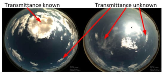
Figure 1.
Sky images of a TSI [9].
Other recent studies [10,11,12] showed that TSI could potentially be used to determine the shading factors for PV applications; nevertheless, this has not been developed yet. For example, ref. [13] proposed a cloud motion estimation using an artificial neural network (ANN). Their model has a relatively low estimation error rate (±5%) and can be used within a broader range of applications.
The approximation of shading in a PV system can also be obtained using the determination of the current-voltage (I-V) curves, applied with maximum power point tracking (MPPT) units [14,15,16]. The problem with these models is that they can predict the amount of loss in the PV output power; however, they cannot indicate the shading factor resulting from the clouds in the sky. In contrast, the output power losses in PV systems can also result from cumulative dust [17], snow [18], hotspots [19,20,21], or cracks [22,23,24,25]. Therefore, assuming that all PV output power losses are caused by shading is substantially incorrect.
Artificial intelligence-based techniques have also recently been applied to approximate the sky’s shading ratio or cloud coverage [26,27]. For example, a recent study [28] demonstrated a cloud cover estimation from images taken by sky-facing cameras using a multi-level machine learning technique. Another recent study [29] explored the applicability of the impact factors to estimate solar irradiance using multiple machine learning algorithms such as support vector machines, a long short-term memory (LSTM) neural network, linear regression, and a multi-layer neural network. They found that the LSTM model provided the best prediction accuracy using weather data without installing and maintaining on-site solar irradiance sensors. In contrast, numerous algorithms have been developed to predict the output power of a typical PV system using weather station data, all of which can be used within a moderately small-scale geographical area of less than 2 km2. When, for example, a location is 20 km apart from the weather station, these algorithms fail to predict the output power accurately; in some cases, even with a closer location (<5 km), it is hard to achieve good prediction results.
2. Aim of This Work
In previous publications, we presented and validated forecasting and predicting shading ratios in a PV system or GHI forecasting from a more comprehensive point of view. However, previous publications did not address the TSI adoption in PV output power forecasting and prediction shading factors expressly within a large-scale area (>20 km2). Therefore, in this article, we aimed to present our work on developing a multi-stage process to accurately approximate the shading ratio of clouds in the sky and apply the method to predict the output power of PV systems. The actual implementation of the algorithm developed was to allocate four TISs within a 25 km2 area and then apply a cloud cover fraction approximation model, named the CA algorithm. Consequently, we predicted the output power of different PV systems within this area. In this article, we also used weather station data to measure the actual GHI and compare it with the obtained GHI from the proposed algorithm; this step was necessary to demonstrate the accuracy of our algorithm.
3. Experimental Setup
Four identical field-mounted TSI 440A total-sky imagers were located in Huddersfield, UK (Figure 2a). TSI-A and TSI-B were 5 km apart; there was also an equivalent distance from TSI-B to TSI-C. It was decided to set up the TSIs in the range of 5 km, as this would give more accurate predictions, since, for example, the Met Office and many researchers propose fixing the TSIs in the field at a distance of 1 to 5 km maximum. The instrument consisted of a spherical mirror and a downward-pointing camera (Figure 2b). For the best image resolution, images had to be taken every 1 min. The camera provided images that were 420 × 420 pixels, which were un-adjustable. Therefore, a cloud identification (filtering) algorithm had to be applied.
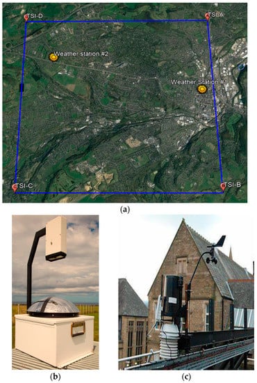
Figure 2.
Experimental setup: (a) Map showing the sky imager locations and the weather stations. The actual distance from TSI-A to TSI-B was 5 km. The region displayed in this figure was approximately 5 km2, taken from @Google Maps, 2022, (b) TSI 440A total-sky imager, (c) Davis weather station.
Two identical Davis weather stations (Figure 2c) were used to validate the accuracy of the shading ratio algorithm. (They will be discussed later in this section). The weather station can measure the solar irradiance in a range of 0–1000 W/m2, with a high accuracy of ±0.5 W/m2. We mounted the weather stations without any slope, as we did for the TSIs.
The data of both the TSIs and the weather stations were taken wirelessly (via cloud-based software) and logged for the duration of the experiments. In addition, the summary of the coordinates of the sites (TSIs and weather stations) are summarized in Table 1.

Table 1.
Site coordinates.
4. Methods
4.1. Cloud Decision Algorithm
To date, the most adaptable cloud estimation algorithms are the blue/red-plus-blue/green-ratio algorithm (BRBG) and the cloud detection and opacity classification algorithm (CDOC). The first algorithm, BRBG, uses the difference in light scattering by clouds compared to a clear-sky day [30]; the result will indicate a factor between 0 and 1, which ultimately describes the cloudiness of an image. On the other hand, the CDOC algorithm is constructed upon the BRBG [31]. This algorithm identifies the cloudiness in the TSI image using the classification of the thickness and the red–blue ratio of the sky image.
The cloud cover fraction (CCF), defined as the fraction of sky covered by clouds, of both algorithms were calculated (Figure 3) for two conditions. In Figure 3a, the CCF equaled 0.58 and 0.76 for BRBG and CDOC, respectively. In this example, the sky was partially covered by thick clouds, covering the sun. In contrast, in Figure 3b, both algorithms had extremely high CCF for the overcasting condition. In this paper, we proposed an adjusted cloud-decision algorithm, and we called it color-adjusted (CA). We can not only determine an accurate measurement for the CCF, but the actual distribution can also be further exaggerated, compared with the BRBG and the CDOC.
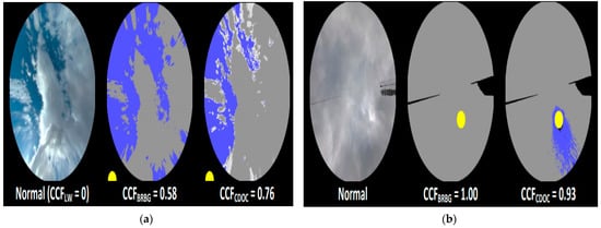
Figure 3.
Evaluation of the CCF ratio for the BRBG and CDOC algorithms under two different shading conditions (note, the yellow cycle represents the actual position of the sun in the sky, and the “normal” is the actual image captured using the full-sky imager): (a) partial shading, (b) overcasting.
The normal image captured using the sky imager was an RGB color image (Figure 4a). The quaternion (red, green, yellow, and blue) pixel values were deposited and combined into a single image, as shown in Figure 4b. Here, the vector of each color was filtered using the hypercomplex convolution,
where is the filtered image in a quaternion array (, is the actual image in quaternion array , is the quaternion left mask , and is the quaternion right mask .
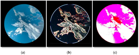
Figure 4.
Evaluation of the proposed cloud decision algorithm: (a) Normal image captured using the full-sky imager, (b) the quaternion values of the image, (c) output image of the CA algorithm (blue–green color ratio); the back area represents CCF ratio = 1.0, blue area represents sky-free, and green is partial clouds.
The cloudiness was observed by selecting the most appropriate color ratio. We found that red–white, Figure 4c, was the most precise color ratio that could instantly discover the clouds, and, therefore, it was used to calculate the CCF.
To verify the differences between our model and the pre-existing models (BRBG and CDOC), the image in Figure 3a was used. The results of our cloud decision algorithm are shown in Figure 4. Initially, the image taken from the TSI was populated into the quaternion values, as shown in Figure 4a, and next, the image color was adjusted to a red–white ratio. Here, the red area represented full shade, the CCF = 1.0, and white or pink (0 being white and 1 being red) represented the free sky (i.e., no, or partial clouds), whereas green was the partial shading area. The CCF value was then calculated by subtracting the ratio of the colors, and we found that in Figure 4c, CCFCA = 0.63, compared with CCFBRBG = 0.58 and CCFCDOC = 0.76. The results of the cloud decision algorithm were in the ranges of the BRBG and CDOC algorithms. However, it is worth noting that the cloud decision algorithm did not take the average values of both algorithms.
4.2. Cloud Cover Fraction Approximation
After completing the CA algorithm, the shading ratio approximation for the selected area was formulated. This approximation aimed to find the shading in the area; that way, the approximation of the cloud coverage can be further improved. First, to identify any position/location on the map, the coordinates of the TSIs must be known, as we have already seen in Figure 2a. If the location of the PV system or the weather station is closer to a particular TSI, the CCF of the TSI will contribute more to the approximation of the shade. This approach is usually referred to as the “adjusted weighted average”. For example, if the weather station was located precisely on the TSI-A location, only the CCF value of the TSI-A would be considered. The distance between the location at and the four TSI locations was calculated using (2), and the sum was calculated using (3), where are the coordinates of the TSIs.
Note that the actual distances were measured in km, where TSI-A was located at (5,5), TSI-B at (5,0), TS-C at (0,0), which in this case, represented the origin of the map, and finally, TSI-D at (0,5).
The contribution of the CCF from each TSI at a particular location were, therefore, calculated based on the ratios of the sum of the distances subtracted by the actual distance from the site, using (4). Then, each CCF contribution was multiplied by the actual CCF, determined using the CA algorithm; consequently, the weighted average CCF was calculated. This was accomplished by calculating the highest two values of the determined CCF contributions.
Let us now consider the weather stations #1 and #2, located at (4.7,3) and (0.8,4), respectively, where the origin was at TSI-C (0,0). The calculations of all the parameters are compiled in Table 2. The optimum distances (shortest) between the weather stations and the actual TSIs are highlighted in the table. The output CCFs at both weather stations were calculated using (5) and (6). The CCF values for the TSIs were taken from Figure 5 (on 15 June 2022 at 11:30).
Table 2.
Results of the parameters with respect to both weather stations.
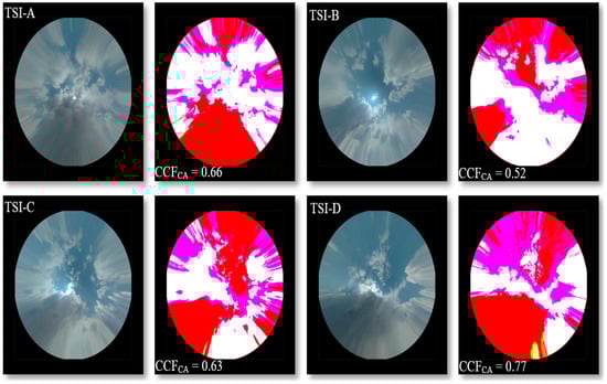
Figure 5.
Normal TSI and the calibrated images using the developed CA algorithm (15 June 2022 11:30).
4.3. Shading Ratio Approximation Flowcode
In summary, the flowcode of the developed shading ratio approximation is presented in Figure 6. Initially, the TSI locations were identified, and then a reference TSI was selected. This corresponded to the actual origin of the map (); this step was critical in measuring the distances of D1, D2, D3, D4, and their sum. Our previous calculation assumed that TSI-C was the origin (Figure 2a).
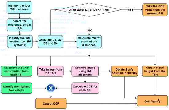
Figure 6.
Flowcode of the developed shading ratio approximation algorithm.
If any of the measured distances were less than or equal to 1 km, the CCF would be taken directly to the adjacent/nearest TSI. This arrangement would give a 97% accuracy of the shade ratio in the location, as empirically evidenced by previous research [32,33,34]. On the other hand, if the location was more than 1 km away from any available TSIs, as with both weather stations in our experiment, the calculations of the CCF contribution and the CCF from the CA algorithm were obtained. Subsequently, the output CCF was determined, corresponding to the actual estimation of the cloud coverage at the site. Therefore, the correlation between the CCF and global horizontal irradiance (GHI) can be obtained using the GHI prediction interval computation models that have been widely presented in literature [35,36,37,38,39]. This depends on three variables: output CCF, sun position in the sky, and the cloud height measured using the TSIs. This step is practically useful when predicting the output power of a PV system (discussed in the next section).
We used the error function as a metric to analyze the performance of the approximation for the GHI; this was calculated using (7).
5. Results
5.1. Accuracy of the Proposed Shading Ratio Approximation Technique
To test the accuracy of the developed technique, we compared the estimated GHI to the actual GHI determined by weather stations #1 and #2 (Figure 7). According to Figure 7a, taken from weather station #1, two conditions were observed on the first day: partial clouds from 6:00–14:00 and clear skies from then onward. We noticed that the error (difference between the actual vs the estimated GHI) was equal to ±7.1% during partial cloud conditions. In contrast, there was a limited error (±2.3%) in the estimated GHI during clear sky conditions.
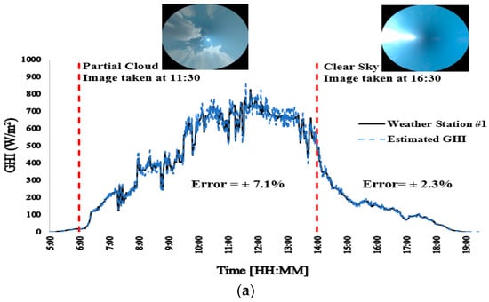
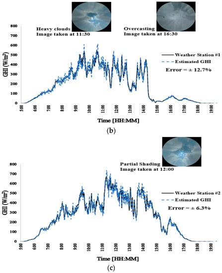
Figure 7.
Output results of the estimated vs actual weather station GHIs under different shading conditions: (a) partial shading and clear sky, taken from weather station #1 (21 July 2022), (b) overcasting (heavy clouds), taken from weather station #1 (22 July 2022), and (c) partial shading, taken from weather station #2 (23 July 2022). (The sky images were taken from the nearest TSI, TSI-A for weather station #1 and TSI-D for weather station #2).
During the second day (Figure 7b), the sky was masked by heavy clouds or what is known as overcasting. This data was taken from weather station #1. In this case, the error in estimating the GHI was ±12.7%. This is likely the case in many cloud estimation techniques [38,39] because, in this specific condition, the sky imager usually fails to measure the height of the clouds precisely, and the output CCF is likely to have a more elevated distribution. In addition, on the third day, and according to Figure 7c, the sky was masked by partial clouds; this measurement was taken from weather station #2. The observed error in the estimation of the GHI was equal to 6.3%.
The above results confirm and validate the idea that the developed algorithm has high accuracy (low error) in estimating the GHI, compared with the actual weather station data.
5.2. Estimating the Output Power of PV Systems
The ultimate aim of the proposed technique is to estimate the shading within an area and hence, predict the output power of PV systems. The advantages here are:
- Weather stations are no longer needed.
- It can predict the shade in relatively large areas (in our case, 25 km2).
- If a high variance is found between the estimated PV power vs the actual measured power in the PV system, a fault identification can be reported.
The temperature of any selected site/location can be taken from the online database available in the Met Office (or simply, using BBC weather as an example in the UK). In this section, to obtain the temperature in the examined PV systems, we used the data available in the Met Office; an update on the temperature can be found in the 5-min resolution, including one-day high-precision measured temperature.
We examined the accuracy of the PV output power estimation using two PV systems located within the studied area (Figure 8a), and the physical images of both PV systems are shown in Figure 8b. PV system #1 was comprised of eight series-connected PV modules and two strings, with a total capacity of 4320 W. PV system #2 also had the same configuration as PV system #1 but with a slightly lower rating power of 3520 W. Neither of the PV systems had a maximum power point tracking unit and were directly connected to the grid via Victron Energy 5 kW inverters that were installed back in May–June 2018. Both systems were maintained, and their data were managed via Solar UK Ltd.; we were given permission to access the data of both PV systems. A loss of 8% in the output power was expected, due to the non-ideal tilt and azimuth arrangements, so we included this ratio in our estimation for the output power.
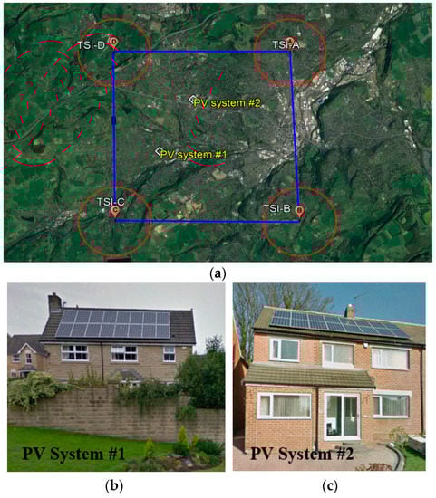
Figure 8.
PV setups: (a) map representing the locations of the examined PV systems and (b,c) physical images of the PV systems.
We followed the same procedure to estimate the GHI in the PV system locations (as detailed in Figure 6). Next, we used (8) and (9) to estimate the output power of the PV systems, where N is the number of solar cells in a PV module (N = 60), and 16 is the total number of PV modules in the system. The parameters 0.00422 and 0.00343 are the equivalent output power of each solar cell, and T0.021 is the weighted temperature.
To summarize the overall performance of the proposed model, we considered plotting the PV output power approximation accuracy against the CCF, presented in Figure 9. We observed that while the CCF was in the range of 0–0.6, the prediction accuracy of the PV output power was above 90%. In contrast, the prediction accuracy decreased when heavy clouds (i.e., overcasting) were present in the sky, and the CCF ratio was above 0.6. In this case, the PV output power prediction accuracy might decrease to as low as 83%.
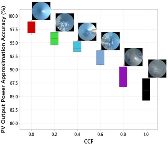
Figure 9.
CCF versus the accuracy of the PV output power prediction.
The actual measured power from the PV systems versus the estimated power using the proposed technique is shown in Figure 10a. The experiment was conducted during a cloudy day, evidenced by the fluctuation in the output power and the actual TSI images taken at 12:00 (Figure 10b). The average temperature of the PV systems is also presented in Figure 10a, taken from the Met Office online database. For PV system #1, the error in estimating the output power was equal to ±3.1%. However, a more significant error was observed when estimating the power of PV system #2, which was ±7.3%. Nevertheless, the developed technique achieved a high accuracy rate in predicting the output power.
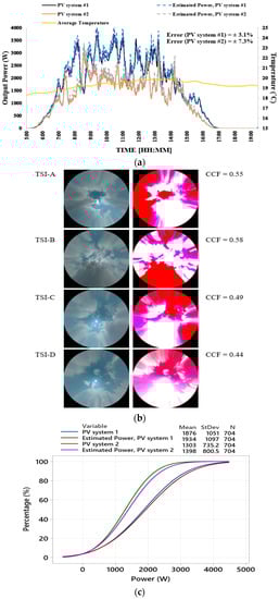
Figure 10.
Output results when using the algorithm with PV systems: (a) output estimated power vs actual measured power in the examined PV systems (03 August 2022), (b) TSI image taken at 12:00, and (c) CDF distribution plot of the data taken from (a).
We further analyzed the data captured during this experiment using a cumulative density function (CDF) distribution, presented in Figure 10c. As a result, we proved a considerable similarity between the actual and the estimated power of both PV systems over the entire spectrum. For example, there was no noticeable difference in predicting the power in low irradiance compared with high irradiance levels. In addition, the standard deviation (StDev) and the mean of the experimental datasets were relatively identical.
6. Comparative Study
This section compares the work presented in this paper against several recently published articles [40,41,42,43]. A summary of the comparisons is presented in Table 3. In [40,41], the authors have presented some interesting results on approximating the GUI and cloud cover, mainly using artificial intelligence-based algorithms. Specifically, in [40], a prediction of the GUI using an LM-BP model was proposed. However, the algorithm appeared more accurate when the solar irradiance was lower than 80–100 W/m2. In addition, ref. [41] proposed a total cloud cover approximation algorithm using a CNN model, yet the proposed solution was unautomated and required intensive human input in the loop. Furthermore, on May 2021, a new paper was published demonstrating how to forecast solar irradiance using an LSTM model. The proposed solution was attractive; however, it needs more clarity on whether the LSTM will work when solar irradiance is under low levels and how far the algorithm can predict solar irradiance from the single-use sky imager. In addition, most recently, in March 2022, authors of [43] demonstrated a new prediction of the solar irradiance algorithm using minute-by-minute images taken with a TSI sky camera. The sky images were taken from the TSI and optimized. However, the algorithm lacked the ability to detect atmospheric attenuation, which resulted in high prediction errors in some instances.
Table 3.
Comparison of this work and previously published papers [40,41,42,43].
In comparison, our algorithm in this paper relied on acquiring four sky images taken from a network of four TSIs. The images were then converted into better quality to identify the clouds/shading in the sky. Our work resulted in a high prediction accuracy of GHI or cloud coverage within 25 km2. More errors are expected from prediction accuracy when the area coverage is increased.
7. Conclusions
This paper presents the development of an approximation for shading using TSI system pictures. The algorithm can estimate the shading ratio in the sky using a color-adjusted processing technique, and subsequently, it can aid in calculating the GHI in the sky. The method was applied to two different PV systems within four TSIs distributed in an area of 25 km2. It was found that, in this case, the GHI can be estimated with a maximum ±12.7% error rate. In addition, the PV output power approximation accuracy was as high as 97.5% when the shading approximation was zero and reduced to the lowest value of 83% when shading was at its maximum. This work can be extended to deploy the developed algorithm in a more comprehensive TSI network, say in an area bigger than 50 km2. This more comprehensive TSI network could further justify the proposed algorithm’s accuracy and support the shading estimation of more PV systems.
Author Contributions
Conceptualization, M.D.; methodology, M.D. and P.I.L.; validation, P.I.L.; formal analysis, M.D.; data curation, M.D. and P.I.L.; writing—original draft preparation, M.D.; writing—review and editing, M.D. and P.I.L. All authors have read and agreed to the published version of the manuscript.
Funding
This research received no external funding.
Conflicts of Interest
The authors declare no conflict of interest.
Abbreviations
The following abbreviations are used in this manuscript:
| PV | photovoltaic |
| CA | color-adjusted |
| GHI | global horizontal irradiance |
| TSI | total-sky imagers |
| ANN | artificial neural network |
| I-V | current-voltage |
| MPPT | maximum power point tracking |
| LSTM | long short-term memory |
| BRBG | blue/red-plus-blue/green-ratio algorithm |
| CDOC | cloud-detection and opacity classification algorithm |
| CCF | cloud cover fraction |
| CDF | cumulative density function |
| StDev | standard deviation |
| CNN | convolutional neural network |
| LM-BP | Levenberg–Marquardt backpropagation |
References
- Su, H.Y.; Liu, T.Y.; Hong, H.H. Adaptive residual compensation ensemble models for improving solar energy generation forecasting. IEEE Trans. Sustain. Energy 2019, 11, 1103–1105. [Google Scholar] [CrossRef]
- Bochenek, B.; Ustrnul, Z. Machine learning in weather prediction and climate analyses—Applications and perspectives. Atmosphere 2022, 13, 180. [Google Scholar] [CrossRef]
- Yang, D.; Wang, W.; Hong, T. A historical weather forecast dataset from the European Centre for Medium-Range Weather Forecasts (ECMWF) for energy forecasting. Sol. Energy 2022, 232, 263–274. [Google Scholar] [CrossRef]
- Zhen, Z.; Zhang, X.; Mei, S.; Chang, X.; Chai, H.; Yin, R.; Wang, F. Ultra-short-term irradiance forecasting model based on ground-based cloud image and deep learning algorithm. IET Renew. Power Gener. 2022, 16, 2604–2616. [Google Scholar] [CrossRef]
- Lee, S.; Kim, G.; Lee, M.I.; Choi, Y.; Song, C.K.; Kim, H.K. Seasonal Dependence of Aerosol Data Assimilation and Forecasting Using Satellite and Ground-Based Observations. Remote Sens. 2022, 14, 2123. [Google Scholar] [CrossRef]
- Yang, D.; Perez, R. Can we gauge forecasts using satellite-derived solar irradiance? J. Renew. Sustain. Energy 2019, 11, 023704. [Google Scholar] [CrossRef]
- Deif, M.A.; Solyman, A.A.; Alsharif, M.H.; Jung, S.; Hwang, E. A hybrid multi-objective optimizer-based SVM model for enhancing numerical weather prediction: A study for the Seoul metropolitan area. Sustainability 2021, 14, 296. [Google Scholar] [CrossRef]
- Yang, H.; Kurtz, B.; Nguyen, D.; Urquhart, B.; Chow, C.W.; Ghonima, M.; Kleissl, J. Solar irradiance forecasting using a ground-based sky imager developed at UC San Diego. Sol. Energy 2014, 103, 502–524. [Google Scholar] [CrossRef]
- Nouri, B.; Wilbert, S.; Segura, L.; Kuhn, P.; Hanrieder, N.; Kazantzidis, A.; Schmidt, T.; Zarzalejo, L.; Blanc, F.; Pitz-Paal, R. Determination of cloud transmittance for all sky imager based solar nowcasting. Sol. Energy 2019, 181, 251–263. [Google Scholar] [CrossRef]
- Kong, W.; Jia, Y.; Dong, Z.Y.; Meng, K.; Chai, S. Hybrid approaches based on deep whole-sky-image learning to photovoltaic generation forecasting. Appl. Energy 2020, 280, 115875. [Google Scholar] [CrossRef]
- Zhen, Z.; Liu, J.; Zhang, Z.; Wang, F.; Chai, H.; Yu, Y.; Lu, X.; Wang, T.; Lin, Y. Deep learning based surface irradiance mapping model for solar PV power forecasting using sky image. IEEE Trans. Ind. Appl. 2020, 56, 3385–3396. [Google Scholar] [CrossRef]
- Nouri, B.; Blum, N.; Wilbert, S.; Zarzalejo, L.F. A hybrid solar irradiance nowcasting approach: Combining all sky imager systems and persistence irradiance models for increased accuracy. Sol. RRL 2022, 6, 2100442. [Google Scholar] [CrossRef]
- Eşlik, A.H.; Akarslan, E.; Hocaoğlu, F.O. Cloud Motion Estimation with ANN for Solar Radiation Forecasting. In Proceedings of the 2021 International Congress of Advanced Technology and Engineering (ICOTEN), Taiz, Yemen, 4–5 July 2021; pp. 1–5. [Google Scholar]
- Dhimish, M. 70% decrease of hot-spotted photovoltaic modules output power loss using novel MPPT algorithm. IEEE Trans. Circuits Syst. II Express Briefs 2019, 66, 2027–2031. [Google Scholar]
- Guerra, M.I.; Ugulino de Araújo, F.M.; Dhimish, M.; Vieira, R.G. Assessing maximum power point tracking intelligent techniques on a pv system with a buck–boost converter. Energies 2021, 14, 7453. [Google Scholar] [CrossRef]
- Dhimish, M. Assessing MPPT techniques on hot-spotted and partially shaded photovoltaic modules: Comprehensive review based on experimental data. IEEE Trans. Electron Devices 2019, 66, 1132–1144. [Google Scholar] [CrossRef]
- Aslam, A.; Ahmed, N.; Qureshi, S.A.; Assadi, M.; Ahmed, N. Advances in Solar PV Systems; A Comprehensive Review of PV Performance, Influencing Factors, and Mitigation Techniques. Energies 2022, 15, 7595. [Google Scholar] [CrossRef]
- Van Noord, M.; Landelius, T.; Andersson, S. Snow-Induced PV Loss Modeling Using Production-Data Inferred PV System Models. Energies 2021, 14, 1574. [Google Scholar] [CrossRef]
- Vieira, R.G.; de Araújo, F.M.U.; Dhimish, M.; Guerra, M.I.S. A Comprehensive Review on Bypass Diode Application on Photovoltaic Modules. Energies 2020, 13, 2472. [Google Scholar] [CrossRef]
- Muteri, V.; Cellura, M.; Curto, D.; Franzitta, V.; Longo, S.; Mistretta, M.; Parisi, M.L. Review on Life Cycle Assessment of Solar Photovoltaic Panels. Energies 2020, 13, 252. [Google Scholar] [CrossRef]
- Olalla, C.; Hasan, M.N.; Deline, C.; Maksimović, D. Mitigation of Hot-Spots in Photovoltaic Systems Using Distributed Power Electronics. Energies 2018, 11, 726. [Google Scholar] [CrossRef]
- Kim, J.; Rabelo, M.; Padi, S.P.; Yousuf, H.; Cho, E.-C.; Yi, J. A Review of the Degradation of Photovoltaic Modules for Life Expectancy. Energies 2021, 14, 4278. [Google Scholar] [CrossRef]
- Dhimish, M.; Mather, P. Ultrafast high-resolution solar cell cracks detection process. IEEE Trans. Ind. Inform. 2019, 16, 4769–4777. [Google Scholar] [CrossRef]
- Libra, M.; Daneček, M.; Lešetický, J.; Poulek, V.; Sedláček, J.; Beránek, V. Monitoring of Defects of a Photovoltaic Power Plant Using a Drone. Energies 2019, 12, 795. [Google Scholar] [CrossRef]
- Goudelis, G.; Lazaridis, P.I.; Dhimish, M. A Review of Models for Photovoltaic Crack and Hotspot Prediction. Energies 2022, 15, 4303. [Google Scholar] [CrossRef]
- Li, Z.; Rahman, S.M.; Vega, R.; Dong, B. A Hierarchical Approach Using Machine Learning Methods in Solar Photovoltaic Energy Production Forecasting. Energies 2016, 9, 55. [Google Scholar] [CrossRef]
- Khandakar, A.; Chowdhury, M.E.H.; Kazi, M.-K.; Benhmed, K.; Touati, F.; Al-Hitmi, M.; Gonzales, A.J.S.P. Machine Learning Based Photovoltaics (PV) Power Prediction Using Different Environmental Parameters of Qatar. Energies 2019, 12, 2782. [Google Scholar] [CrossRef]
- Park, S.; Kim, Y.; Ferrier, N.J.; Collis, S.M.; Sankaran, R.; Beckman, P.H. Prediction of Solar Irradiance and Photovoltaic Solar Energy Product Based on Cloud Coverage Estimation Using Machine Learning Methods. Atmosphere 2021, 12, 395. [Google Scholar] [CrossRef]
- Cha, J.; Kim, M.K.; Lee, S.; Kim, K.S. Investigation of Applicability of Impact Factors to Estimate Solar Irradiance: Comparative Analysis Using Machine Learning Algorithms. Appl. Sci. 2021, 11, 8533. [Google Scholar] [CrossRef]
- Esteves, J.; Cao, Y.; da Silva, N.P.; Pestana, R.; Wang, Z. Identification of clouds using an all-sky imager. In Proceedings of the 2021 IEEE Madrid PowerTech, Madrid, Spain, 28 June–2 July 2021; pp. 1–5. [Google Scholar]
- Pu, R.; Landry, S.; Zhang, J. Evaluation of atmospheric correction methods in identifying urban tree species with WorldView-2 imagery. IEEE J. Sel. Top. Appl. Earth Obs. Remote Sens. 2014, 8, 1886–1897. [Google Scholar] [CrossRef]
- Logothetis, S.-A.; Salamalikis, V.; Nouri, B.; Remund, J.; Zarzalejo, L.F.; Xie, Y.; Wilbert, S.; Ntavelis, E.; Nou, J.; Hendrikx, N.; et al. Solar Irradiance Ramp Forecasting Based on All-Sky Imagers. Energies 2022, 15, 6191. [Google Scholar] [CrossRef]
- Zuo, H.M.; Qiu, J.; Jia, Y.H.; Wang, Q.; Li, F.F. Ten-minute prediction of solar irradiance based on cloud detection and a long short-term memory (LSTM) model. Energy Rep. 2022, 8, 5146–5157. [Google Scholar] [CrossRef]
- Du, J.; Min, Q.; Zhang, P.; Guo, J.; Yang, J.; Yin, B. Short-term solar irradiance forecasts using sky images and radiative transfer model. Energies 2018, 11, 1107. [Google Scholar] [CrossRef]
- Zhang, X.; Fang, F.; Wang, J. Probabilistic solar irradiation forecasting based on variational Bayesian inference with secure federated learning. IEEE Trans. Ind. Inform. 2020, 17, 7849–7859. [Google Scholar] [CrossRef]
- Zhang, R.; Ma, H.; Hua, W.; Saha, T.K.; Zhou, X. Data-driven photovoltaic generation forecasting based on a Bayesian network with spatial–temporal correlation analysis. IEEE Trans. Ind. Inform. 2019, 16, 1635–1644. [Google Scholar] [CrossRef]
- Andrade, J.R.; Bessa, R.J. Improving renewable energy forecasting with a grid of numerical weather predictions. IEEE Trans. Sustain. Energy 2017, 8, 1571–1580. [Google Scholar] [CrossRef]
- Jiang, H.; Gu, Y.; Xie, Y.; Yang, R.; Zhang, Y. Solar irradiance capturing in cloudy sky days–a convolutional neural network based image regression approach. IEEE Access 2020, 8, 22235–22248. [Google Scholar] [CrossRef]
- Kumar, U.; Sahoo, B.; Chatterjee, C.; Raghuwanshi, N.S. Evaluation of simplified surface energy balance index (S-SEBI) method for estimating actual evapotranspiration in Kangsabati reservoir command using landsat 8 imagery. J. Indian Soc. Remote Sens. 2020, 48, 1421–1432. [Google Scholar] [CrossRef]
- Crisosto, C.; Hofmann, M.; Mubarak, R.; Seckmeyer, G. One-Hour Prediction of the Global Solar Irradiance from All-Sky Images Using Artificial Neural Networks. Energies 2018, 11, 2906. [Google Scholar] [CrossRef]
- Krinitskiy, M.; Aleksandrova, M.; Verezemskaya, P.; Gulev, S.; Sinitsyn, A.; Kovaleva, N.; Gavrikov, A. On the Generalization Ability of Data-Driven Models in the Problem of Total Cloud Cover Retrieval. Remote Sens. 2021, 13, 326. [Google Scholar] [CrossRef]
- Rajagukguk, R.A.; Kamil, R.; Lee, H.-J. A Deep Learning Model to Forecast Solar Irradiance Using a Sky Camera. Appl. Sci. 2021, 11, 5049. [Google Scholar] [CrossRef]
- Alonso-Montesinos, J.; Monterreal, R.; Fernandez-Reche, J.; Ballestrín, J.; López, G.; Polo, J.; Barbero, F.J.; Marzo, A.; Portillo, C.; Batlles, F.J. Nowcasting System Based on Sky Camera Images to Predict the Solar Flux on the Receiver of a Concentrated Solar Plant. Remote Sens. 2022, 14, 1602. [Google Scholar] [CrossRef]


Publisher’s Note: MDPI stays neutral with regard to jurisdictional claims in published maps and institutional affiliations. |
© 2022 by the authors. Licensee MDPI, Basel, Switzerland. This article is an open access article distributed under the terms and conditions of the Creative Commons Attribution (CC BY) license (https://creativecommons.org/licenses/by/4.0/).