Article

Modeling of Photovoltaic Array Based on Multi-Agent Deep Reinforcement Learning Using Residuals of I–V Characteristics

1
College of Mechanical and Electrical Engineering, Hohai University, Changzhou 213022, China
2
Solar Computing Laboratory, University of Applied Sciences Bielefeld, Artilleriestraße 9, 32427 Minden, Germany
3
Engineering Research Center of Dredging Technology of Ministry of Education, Changzhou 213022, China
4
School of Physics and Electronic Electrical Engineering, Huaiyin Normal University, Huai’an 223300, China
*
Author to whom correspondence should be addressed.
Energies 2022, 15(18), 6567; https://doi.org/10.3390/en15186567
Submission received: 25 July 2022 / Revised: 1 September 2022 / Accepted: 4 September 2022 / Published: 8 September 2022

Abstract

:
Currently, the accuracy of modeling a photovoltaic (PV) array for fault diagnosis is still unsatisfactory due to the fact that the modeling accuracy is limited by the accuracy of extracted model parameters. In this paper, the modeling of a PV array based on multi-agent deep reinforcement learning (RL) using the residuals of I–V characteristics is proposed. The environment state based on the high dimensional residuals of I–V characteristics and the corresponding cooperative reward is presented for the RL agents. The actions of each agent considering the damping amplitude are designed. Then, the entire framework of modeling a PV array based on multi-agent deep RL is presented. The feasibility and accuracy of the proposed method are verified by the one-year measured data of a PV array. The experimental results show that the higher modeling accuracy of the next time step is obtained by the extracted model parameters using the proposed method, compared with that using the conventional meta-heuristic algorithms and the analytical method. The daily root mean square error (RMSE) is approximately 0.5015 A on the first day, and converges to 0.1448 A on the last day of training. The proposed multi-agent deep RL framework simplifies the design of states and rewards for extracting model parameters.

1. Introduction

As an important form of renewable energy, solar photovoltaic (PV) systems have developed rapidly in the last decade. In the recent report of International Energy Agency (IEA), China is likely to account for almost half of the global increase in renewable electricity generation, with over 900 TWh from solar PV and wind in 2021 [1]. The huge renewable energy market attracts more attention on the intelligent operation and maintenance and fault diagnosis technology of the PV systems, which can directly enhance the efficiency and reduce the labor cost of maintenance. As the first-level energy conversion devices in the PV systems, the PV array directly converts solar energy into electrical energy and suffers long-term outdoor uncertain meteorological factors, e.g., thermal cycles, ultraviolet radiation, dust, and hail. Therefore, in recent years, many researchers have carried out the study of the fault detection and diagnosis (FDD) of the PV array [2,3]. The model-based FDD methods are proposed to diagnose most faults or abnormalities, e.g., open-circuit, line-line or line-ground short-circuit fault of the PV array [4,5,6], cable aging or series impedance abnormality [7,8], partial shading [8,9,10,11], etc. For the FDD of the PV arrays, the modeling of the PV array is required [8,9,10]. The greater modeling error may also lead to the misdiagnosis of the PV array. Additionally, the online FDD of the PV array has a higher requirement for the real-time performance of modeling. Thus, it challenges the accuracy and adaptivity of the mathematical model under various ambient conditions. Unfortunately, the conventional modeling methods cannot satisfy the accuracy and real-time demands for FDD.
Commonly, the mathematical models of PV array are derived from the equivalent single-diode model (SDM), double-diode model (DDM), or multi-dimension diode model of solar cells. Then, the I–V curves of the PV array can be estimated based on the measured irradiance on the plane of the PV array and module temperature after extracting the model parameters [7,12,13,14,15,16]. At present, the model parameter extracting methods can be divided into two main categories. One is to analytically or numerically solve the model parameters based on the measured or rated electrical parameters of PV modules, commonly provided by manufacturers [7,12]. In [12], the equation to estimate the temperature coefficient of voltage is proposed to build the equation systems and to solve the model parameters. In [7], the explicit methods to solve the model parameters are analyzed to detect the degradation of the PV module. However, few methods exhibit acceptable accuracy and reliability to estimate the model parameters. Nevertheless, the model parameters may vary with the change of the ambient irradiance or temperature conditions. The model parameter, e.g., series resistance and ideal factor, are considered as constants which may deteriorate the accuracy of the model.
Another category of parameter extraction attempts to minimize an objective function, which represents the error between the measured I–V curve and the modeled one. Then, the model parameters are extracted by the meta-heuristic optimizers [13,14,15,16,17,18,19], e.g., particle swarm optimizer (PSO) [8], culture algorithm (CA) [17], and artificial bee colony (ABC) [18]. This category of methods uses the data points on the entire measured I–V curve. The accuracy of modeling is much higher than that of the analytical method. At present, some PV inverter products have the capability to measure the I–V curves of PV arrays, which makes the above methods suitable for applications, e.g., the FDD. However, the referenced I–V curve at each time step of diagnosis should be modeled based on the optimized model parameters. Thus, the meta-heuristic optimizers cannot estimate the variation in model parameters. In addition, some researchers have directly used the supervised learning algorithms to model the PV array, e.g., by training a one-dimensional deep residual network [20]. To ensure the good generalization of the network, the training samples under different irradiation and temperature levels are required [20]. Once the above model is applied to the fault diagnosis of PV arrays, the samples should be periodically updated, and the model needs be retrained to ensure the long-term stability of the model accuracy. In recent years, reinforcement learning (RL) has been applied in the electrical power engineering area. The RL is a machine learning process that leads the RL agents to interact with the designed environment by constructing a Markov decision process (MDP). The optimal action strategies are gradually learned based on the feedback of the environment state and the rewards of corresponding actions. Thus, the RL can be used as a self-learning approach, which is quite different from the conventional supervised or unsupervised learning models. The multi-agent RL is commonly used for solving cooperative or adversarial scenarios. The cooperative tasks are realized by evaluating the action of each agent according to the unified and observable environment state and collaborative rewards. Then, the overall optimal action strategy can be obtained after multi-agent collaboration.
In this paper, the modeling of a PV array based on the multi-agent deep RL is proposed. The novelty of this paper is that the RL agents can dynamically adjust the model parameters considering the variation of the ambient conditions for the PV array. The contribution of this paper includes:
  • The design of the states and rewards of the RL agents in the modeling process are simplified for the researchers in PV engineering. The conventional methods for designing the states and rewards of the RL agents are commonly relied in the design of a virtual training environment to interact with RL agents and train them. The design of the states and rewards are according to the virtual training environment [21]. In this paper, the designed states of the RL agents are in terms of the variation of I–V characteristics in the training process, and the reward is designed according to the modeling error of I–V characteristics. For the researchers in PV engineering, the understanding of the modeling process in this paper is easier.
  • The continuous state space is designed for training the RL agents by considering the continuous variation of I–V curves, which can enhance the generalization of the RL agents for estimating variation of model parameters.
At first, the state of the art for the model parameter extraction is briefly reviewed. The mathematical model of the PV array is introduced. Then, the double deep Q network (DDQN) is designed as the value network of the RL model. The multi-agent deep RL framework for the modeling of the PV array is proposed, including the RL states based on the high dimensional residuals of I–V characteristics, multi-agent cooperative rewards, and the agent actions with the damping amplitude. The measured annual I–V curves of a PV array are used to verify the modeling accuracy of the proposed method. Due to the fact that most model parameters extraction methods are currently based on meta-heuristic algorithms, the model estimation results using the model parameters extracted by different meta-heuristic and analytical methods are compared. Finally, the time cost of different model parameter extraction methods are investigated.
This paper is organized as follows: Section 1 briefly reviews the state of the art of model parameter extraction. Section 2 explains the mathematical model of the PV array used in this paper. The proposed modeling method of the PV array based on multi-agent deep RL is presented in Section 3. Section 4 elaborates the experimental verification of the proposed method using the measured data of an actual PV array. Section 5 summarizes the conclusions of this paper.

2. Mathematical Model of PV Array

PV arrays are usually composed of PV modules connected in series and parallel, and each PV module is composed of solar cells connected in series. The bypass diodes are connected in anti-parallel to alleviate the hot spot effect when the cells are mismatched [7]. The physical model of the PV module is commonly described by the SDM, and the corresponding I–V equation is [8]:
I P V = I p h I s exp q ( V P V + R s I P V ) a k T 1 V P V + R s I P V R s h
where I P V and V P V are the output current and voltage of the PV module, respectively; q , k , T are the electronic charge (1.60217662 × 10 19 C), the Boltzmann constant (1.38064852 × 10 23 JK 1 ) and the temperature of the solar cell (in K), respectively. I p h , I s , a , R s , R s h are the five parameters of the mathematical model, which represents the photocurrent, the saturation current of the diode, the ideal factor of diode, the equivalent series, and shunt resistance, respectively. Among them, the photocurrent I p h can be estimated by the irradiation G on the plane of the PV array [8]:
I p h = I S C , s t c 1 + K i ( T T s t c ) G G s t c
I S C , s t c is the short-circuit current of the PV module under the standard test conditions (STC), K i is the temperature coefficient of the current, which can be obtained from the specification of the PV module. G s t c and T s t c are the irradiance (1000 W/m 2 ) and temperature (25 C) under STC, respectively. The saturation current of diode I s can be estimated by the ideal factor of diode a and the temperature T [8]:
I s = I s , s t c T T s t c 3 a exp q E g a k T s t c q E g a k T
E g is the band gap energy, I s , s t c is the saturation current of diode under the STC, which can be expressed as [8]:
I s , s t c = I S C , s t c exp q V O C , s t c N c s a k T s t c 1
where V O C , s t c is the open-circuit voltage of the PV module under STC, and N c s is the number of cells connected in series of the PV module.
Therefore, only the three model parameters, i.e., the ideal factor of diode a, the equivalent series resistance R s and the equivalent parallel resistance R s h should be determined. Then, substituting the model parameters into (1), the I–V equation of the PV module can be established. The model of the PV array can be obtained by multiplying the current and voltage of the PV module with the corresponding number of modules connected in series and parallel. Additionally, considering the measurement error of the pyranometer, a compensation value of irradiance Δ G is introduced as an additional model parameter to correct the measured co-plane irradiance G m e a s :
G = G m e a s + Δ G
The above equations show that the accuracy of the model estimated I–V curve is directly influenced by the extracted model parameters, i.e., the ideal factor of diode a, the equivalent series resistance R s and the equivalent parallel resistance R s h . The output current can be estimated by the corresponding voltage once the irradiance and temperature are known.

3. Modeling of PV Array Based on Multi-Agent Deep Reinforcement Learning

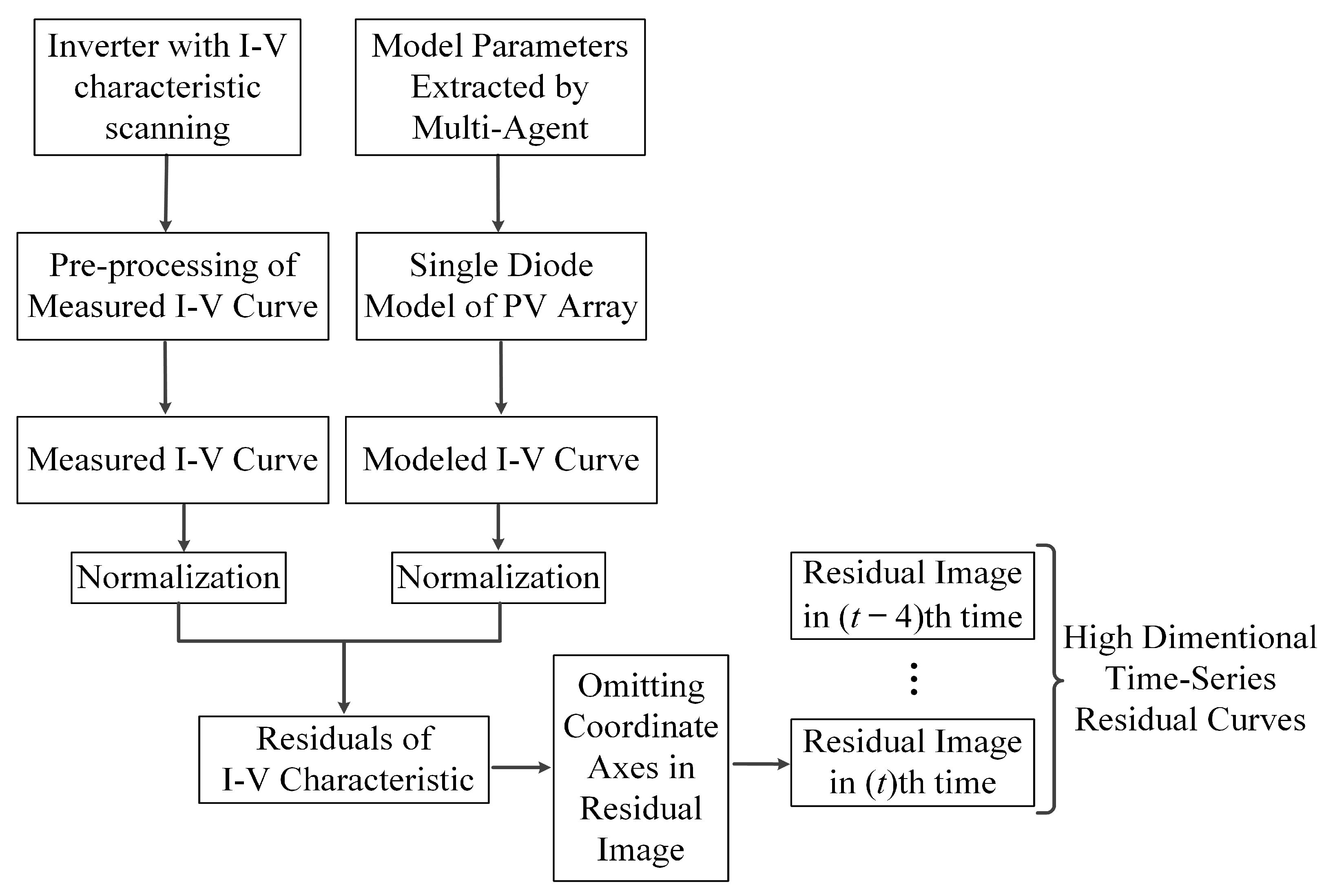
3.1. Design of State and Reward Based on Residuals of I–V Characteristics

In this paper, a multi-agent deep RL framework is proposed for modeling the PV array considering the continuous variation of RL states. In the MDP, the environment state represents the environment change after the act of all agents in the previous time step, i.e., episode. During the extraction of the model parameters, the I–V curves of the PV array can be modeled based on the model parameters estimated by the agents, then the residuals of the modeled I–V curve relative to the measured one are used as the environment state. In this paper, the RL environment state is proposed based on the time-series images of the residual curves of I–V characteristics. Figure 1 represents the flowchart for constructing the environment state of multi-agent deep RL.
At first, the model parameters output by the multi-agent are used to estimate the I–V curve of the PV array according to (1)–(4). The I–V curve measured by the inverter is pre-processed and normalized. Then, the residual value of the current at the same voltage point on the I–V curve is calculated to obtain the residual I–V curve image, and the auxiliary information in the image is removed to form a 160 × 120 pixel image. Considering the time-varying trend of the residual curves during the RL process of the multi-agent, the residual curve images of the latest t 4 to t time step are combined into the 4 × 160 × 120 high-dimensional residuals of I–V characteristics in the time step t, which represents the environment state for training the multi-agent. Obviously, if the value of the current on the residual curve tends towards 0, this indicates that the modeled I–V curve using the parameters estimated by the action of the multi-agent are consistent with the measured I–V curve at time step t, i.e., the modeling accuracy is high sufficient. Due to the residuals of the I–V characteristic being represented by a curve in the image, the lesser resolution is selected. To accurately represent the residuals of the I–V characteristic, the 160 × 120 resolution is enough. The time steps from the latest t 4 to t is chosen according to the fact that the convergence of the DDQN model is more stable if using the latest four time steps [22]. Furthermore, the root mean square error (RMSE) of the current between the estimated and measured I–V curves is used as the criterion for evaluating the effectiveness of the multi-agent actions:
RMSE = 1 N p o i n t s i = 1 N p o i n t s I m o d e l , i I m e a s , i I m e a s , i 2
where N p o i n t s is the number of points on the I–V curve, and I m o d e l , i and I m e a s , i are the estimated and measured value at the i-th point in the I–V curve, respectively. Additionally, the mean absolute error (MAE) and mean absolute percentage error (MAPE) are used to assess the model accuracy during verification:
MAE = 1 N p o i n t s i = 1 N p o i n t s I m o d e l , i I m e a s , i
MAPE = 1 N p o i n t s i = 1 N p o i n t s I m o d e l , i I m e a s , i I m e a s , i
In order to ensure the convergence of the model parameters estimated by the multi-agent, the multi-agent collaborative rewards are designed according to the gradient descent to guarantee the RMSE converging. Therefore, the multi-agent collaborative reward is designed as:
= + 1 , RMSE t RMSE t 1 1 , RMSE t > RMSE t 1
when the RMSE at time step t decreases or keeps the same value as that at the previous time step t 1 , the reward is set as 1, otherwise the reward is −1.

3.2. Design of Actions Considering Amplitude Attenuation

For the accurate parameter extraction and modeling, the designed action should be able to directly estimate the model parameter of the next time step. In this paper, multiple independent agents are used to estimate the corresponding model parameters. The three actions of each agent for the model parameters are designed as follows [23]:
M t + 1 = M t + r M s t c M t + 1 = M t M t + 1 = M t r M s t c M { a , R s , R s h , Δ G } M s t c { a s t c , R s , s t c , R s h , s t c , Δ G s t c }
where a s t c , R s , s t c and R s h , s t c are the corresponding initial model parameters of a , R s , R s h under the STC, respectively, solved by the module of the PV array in MATLAB/Simulink based on the specification of the PV module [24]. Δ G s t c is changing in the range of 1–2% of irradiance under the STC. r is the ratio to turn the amplitude during the RL. At the beginning of the RL, the model parameters should be explored in a greater range. Furthermore, the model parameters should be kept as stable as possible after the RMSE converges. Considering that, the total RL time step is at least 10,000 steps, r is designed to decay with the RL time step t as the trend of sigmoid function:
r = 0.02 0.01 1 + exp t 500 10 , t 10 , 000 0.01 , t > 10 , 000
As shown in Figure 2, at the beginning of the training, the r is greater and the adjustment step for each model parameter is approximately 2% of the model parameters under STC, i.e., a s t c , R s , s t c , R s h , s t c and G s t c . This mechanism can promote the RL agents to explore the action space and enhance the diversity of the replay memory. After approximately 4000 time steps, the adjustment step of each model parameter is gradually reduced towards 1%, and a more stable action selection strategy is used after the Q network is converged.

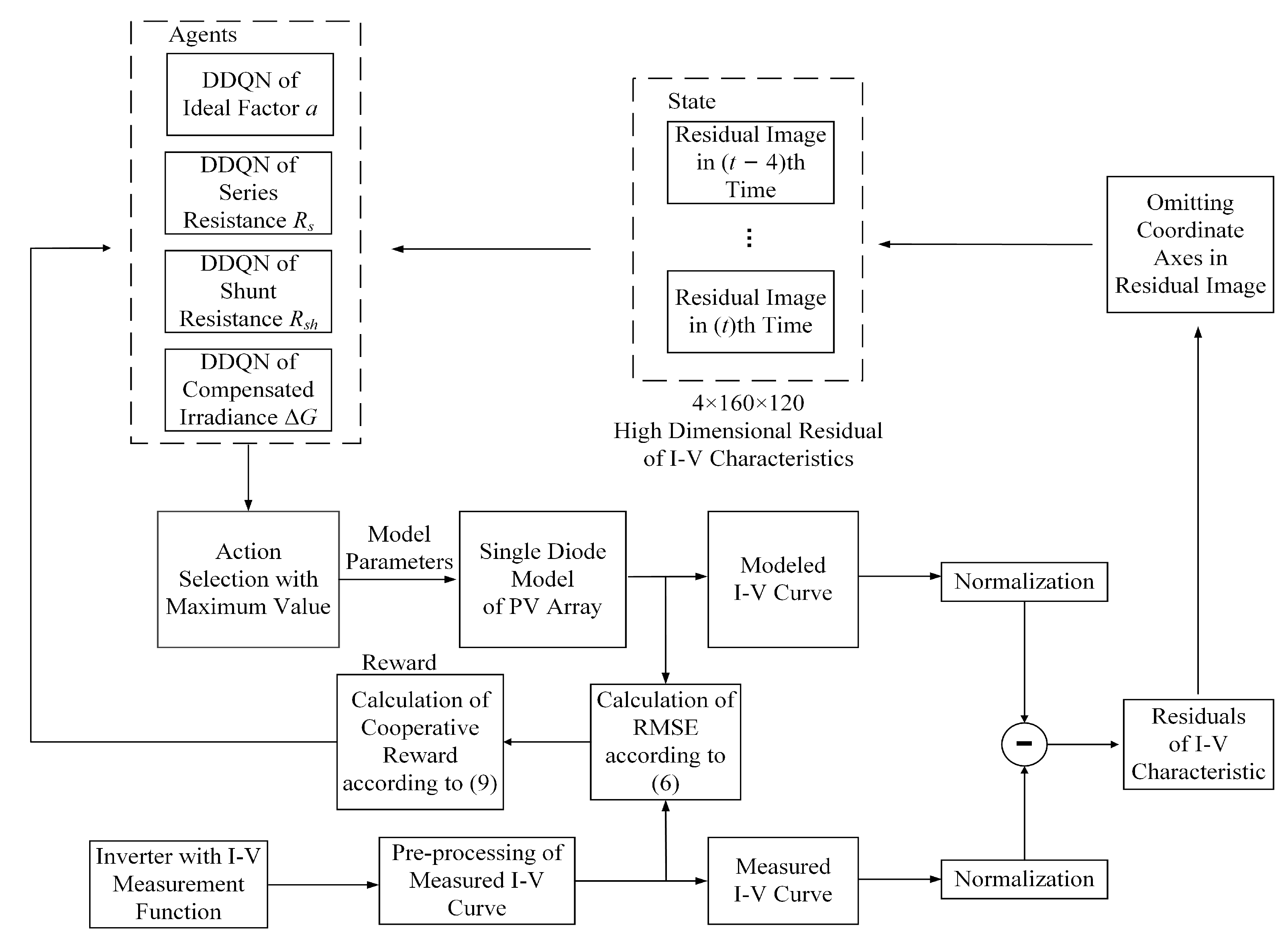
3.3. Agents Based on Double Deep Q Network

The DDQN originates from the double Q-learning algorithm [21]. Similarly to the deep Q network, the DDQN improves the description of the value function of action policy using a deep Q-value network, instead of the Q-table. The advantage of DDQN is that the continuous changes in the environment state are considered, and high-dimensional continuous state input can be realized [22]. In the DDQN, the evaluation Q-network with the network weight set θ is used to determine the value function of the action a t under the environment state s t at the current time step t, which is denoted as Q ( s t , a t ; θ ) . Then, the target Q-network is used to estimate the target Q-value Q ( s t + 1 , a t + 1 ; θ ) of the next state s t + 1 at the next time step. The network weight set θ of the evaluation Q-network is trained by the adaptive moment estimation (ADAM) algorithm and the network loss function L ( θ ) is minimized, which is defined as [21,22]:
L ( θ ) = E + γ Q ( s t + 1 , arg max a t + 1 Q ( s t + 1 , a t + 1 ; θ ) , θ ) Q ( s t , a t ; θ ) 2
where γ is the discount factor taking values between (0,1), and E represents the mathematical expectation of the error. θ is the network parameter set for the target Q network. A batch of samples are randomly selected from the experience replay memory to train the current network [21,22]. After the evaluation, Q-network is trained, and the target Q-network can be periodically updated by the evaluation Q-network. Then, the target Q-value is estimated by the target Q-network to realize the further training of the evaluation Q-network.
The deep convolutional networks are the type of networks most commonly used to identify patterns in images. Considering the designed environment state based on the residuals of I–V characteristics, the deep convolutional network is used as the Q-network of each agent, due to its fast training and ability to capture the local features of images [25,26,27]. The network structure is shown in Figure 3. At first, the 4 × 160 × 120 high-dimensional residuals of I–V characteristics are fed into the convolutional network with three 20 × 20 filters, and the rectified linear unit (ReLU) is used as the activation function to form a 3 × 15 × 11 matrix. Then, the 4 × 4 averaging pooling is connected to form a 3 × 3 × 2 matrix, which is further flattened into an 18 × 1 vector. Finally, the vector is fed to the fully connected layer with the sigmoid activation function to obtain the estimated value of the actions for each agent. The action with the estimated maximum value is selected as the final action.

3.4. Modeling Framework of PV Array Based on Multi-Agent Deep RL

The proposed modeling framework of the PV array based on the multi-agent deep RL is shown in Figure 4. At first, the I–V curves of the PV array measured by the inverter and the I–V curve estimated by the model are compared to construct the residuals of I–V characteristics, which is used as the environment state to train each agent of the model parameter. Then, the RMSE of the I–V curve is calculated via (6), and the multi-agent cooperative reward is obtained via (9). Additionally, the loss function of the Q network is optimized by the ADAM algorithm, and the residuals of I–V characteristics are fed to the DDQN of each agent to estimate the result of value function. After determining the optimal action strategy, the model parameters can be estimated via (10). Then, the model parameters are obtained and input to the mathematical model of the PV array to estimate the I–V curve at the next time step, based on the measured in-plane irradiance and module temperature. Finally, the model parameter extraction and modeling of the PV array is realized.

4. Experimental Verification of Proposed Method Based on Multi-Agent Deep Reinforcement Learning

In order to verify the accuracy of the proposed method based on multi-agent deep RL, a 5.28 kWp PV array, formed by 22 multi-crystalline PV modules TSM-240, is used for experimental verification. The specification of the PV module TSM-240 under STC provided by the manufacturer is shown in Table 1. The PV system is equipped with the three-phase grid-connected inverter GW20KN-DT, which can measure the I–V curves of the PV array. At least 256 points on the I–V curve can be measured in 2 s. The pyranometer TBQ-2 is used to measure the in-plane irradiance of the PV array. The platinum resistors Pt100 are pasted on the back sheet of the PV modules to measure the temperature of PV module. I–V curves of the PV array, in-plane irradiance, and temperature of the PV module are transmitted via the RS485 bus to an indoor monitor computer with proposed modeling method. Data measured from 27 June 2018 to 31 July 2019 are used for verification. Considering that the measured I–V characteristic of the PV array may lead to the power loss of the PV plant, the measurement and modeling cannot be too frequent. However, the total number of training samples should be guaranteed, as a greater time interval leads to longer training duration. Therefore, the time interval should be determined in a trade-off. In the experiments, the measurement interval is 2 min. The measured I–V curves are pre-processed. The data measured with the irradiation less than 200 W/m 2 are neglected to reduce the influence of measurement errors. Additionally, the distorted I–V curves or data measured under the mismatch conditions of the PV array, e.g., the partial shading or other abnormalities, are filtered to ensure that the RL multi-agent are trained with normal samples. The number of local maximum and minimum on the second order derivative curve d 2 I / d V 2 is used as an indicator to identify these abnormal I–V curves [8]. Then, the proposed multi-agent deep RL-based method is used to estimate the model parameters of the next time step. The modeling accuracy of the proposed method is statistically analyzed and compared with the conventional or recently presented model extraction methods, including the particle swarm optimizer (PSO) [8], culture algorithm (CA) [17], and analytical method [12]. The modeling accuracy of the next time step, using the above different parameter extraction methods, are focused upon herein.
Figure 5 shows the histogram of the annual accuracy comparison of modeling the I–V curve at the next time step based on the model parameters extracted by the proposed method and other algorithms. The annual RMSEs of the proposed method converge to approximately 0.1 A. The proposed multi-agent deep RL-based method shows better performance for modeling the I–V curves at the next time step, compared with the PSO, CA, or the analytical method. The reason for which the meta-heuristic algorithms or the analytical method fail is that, the meta-heuristic optimizers only use the measured I–V curve at the current time step to extract the model parameters, and can only guarantee the accuracy of modeling at the current time step. This may cause difficulty in accurately modeling for the (t + 1)-th time step. The dynamic change of model parameters cannot be considered. However, once the loss function of DDQN is converged, the proposed multi-agents can select the correct action to regulate the model parameters according to the residuals of I–V characteristics by training the DDQN. Thus, more accurate model parameters can be estimated for the next time step, which enhances the adaptability of the modeling. Figure 6 shows the moving average of 20 adjacent values of the RMSE and corresponding fitted trend line. Due to the fact that the initial date is approximately in early July 2018, the trend of the RMSE shows that the RL agents basically converge in the beginning of December 2018, which is approximately 5 months. The RMSE is disconnected due to the data missing or filtering of the abnormal measured I–V curves. The convergence can be accelerated if more I–V curves are measured to train the RL agents, or increasing the sample frequency of the I–V characteristics.
The average RMSEs of different methods in typical dates of the entire RL period are listed in Table 2. On the first day, i.e., 27 June 2018, the daily average RMSE of modeling using the multi-agent deep RL-based method is approximately 0.5015 A. The RMSE is even higher than that of the other meta-heuristic methods. The reason is that the training of DDQN is not completed. The RMSE of the proposed method converges to 0.1448 A in the last day of verification, i.e., 31 July 2019. However, for the PSO-based and CA-based methods, the daily RMSEs show no obvious convergence trend. Similar results can also be observed from Figure 5.
Table 3 shows the annual MAE, RMSE, and MAPE for different methods. The annual MAE of the proposed method is 0.24 A and is approximately 2.44% of the short-circuit current of the PV array under the STC. The annual MAPE of the proposed method is approximately 12.20%, which is acceptable for modeling a PV array, considering the fact that the error is relatively greater when the training process of DDQN is uncompleted.
Figure 7 presents the comparison results between the measured and the modeled I–V curves based on the above parameter extraction methods in the typical days of four seasons. The estimation results of the multi-agent deep RL-based method obtains greater errors compared with the measured I–V curves in Figure 7a due to the insufficient training samples and un-converged DDQN for the proposed method. However, Figure 7b–d show that the modeling results of the proposed method are more consistent with the measured curves. Compared with the conventional meta-heuristic methods for estimating the model parameters of the next time step, the proposed method obtains a better modeling accuracy under lower irradiation levels, e.g., approximately 200 W/m 2 . Table 4 and Table 5 list the calculated MAE and MAPE for each I–V curve in Figure 7, using different modeling methods. The same results can be observed that the proposed multi-agent deep RL-based method does not perform well in 28 September 2018. It results in more uncertain model parameters and reduces the modeling accuracy. With the training of RL agents, the MAE and MAPE both show that the performance of the proposed method is significantly enhanced.
Additionally, the PSO-based and CA-based method both obtain greater MAE or MAPE. Similar conclusions can also be observed from Figure 7. The reason is that, for these meta-heuristic methods, the model parameters are extracted using the measured I–V curve at the latest time step. The assumption that the model parameters would not change significantly between two adjacent time steps is a necessary precondition. However, for the actual outdoor circumstance, the ambient irradiance may vary randomly according to the actual meteorological conditions. Thus, the above assumption is not always valid, which causes the lower accuracy of the meta-heuristic methods. For the proposed multi-agent deep RL-based method, the RL agents attempt to regulate the model parameters towards more suitable values, according to the residuals of I–V characteristics. Once the DDQN is trained with enough samples, then better accuracy can be obtained.
Figure 8 shows the time consumption of model parameter extraction using the proposed multi-agent deep RL-based method and other methods. The parameter extraction programs are executed on the same PC with Intel(R) Core(TM) i7-6700HQ CPU (@2.60 GHz, eight cores) and 8 GB memory, without GPU acceleration. The PSO-based method is faster than other methods. The average time cost of the proposed multi-agent deep RL-based method is approximately 2.343 s, which is similar to that of the CA-based method. The most time is consumed by computing the DDQN. However, it should be pointed out that the computation of DDQN can be accelerated using the GPUs, and the time cost of the proposed multi-agent deep RL-based method can be further reduced.

5. Conclusions

In this paper, a multi-agent deep RL framework is proposed for estimating the model parameters and modeling the PV array in the next time step. The environment state based on the high-dimensional residuals of I–V characteristics and a corresponding cooperative reward is presented for the RL agents. The actions of each agent considering the damping amplitude are designed. Then, the entire framework of modeling of PV array based on multi-agent deep RL is presented. The feasibility and accuracy of the proposed method are verified by the one year measured data of a PV array. The experimental results show that the higher modeling accuracy of the next time step is obtained by the extracted model parameters using the proposed method, compared with that using the conventional meta-heuristic algorithms and the analytical method. The daily root mean square error (RMSE) is approximately 0.5015 A in the first day, and converges to 0.1448 A in the last day of training. The time consumption of model parameter extraction using the proposed multi-agent deep RL-based method is approximately 2.343 s by using a PC without GPU acceleration. The time cost could be further reduced if the GPU acceleration is utilized.
Future research should focus on enhancing the convergence speed of the proposed multi-agent deep RL-based method. Another aspect would be to optimize the network structure and corresponding hyper-parameters. The proposed modeling approach would be considered to embed in the existing FDD platform for the intelligent operation and maintenance of the PV array.

Author Contributions

Conceptualization, J.Z. and Z.Y.; methodology, J.Z.; software, J.Z. and Z.Y.; validation, J.Z. and Z.Y.; formal analysis, J.Z. and L.F.; investigation, X.C. and L.C.; resources, Y.L.; data curation, J.Z. and Z.Y.; writing—original draft preparation, J.Z. and Z.Y.; writing—review and editing, J.Z., K.D. and F.H.; visualization, J.Z. and Z.Y.; supervision, K.D. and F.H.; project administration, K.D. and F.H.; funding acquisition, J.Z., X.C., K.D. and F.H. All authors have read and agreed to the published version of the manuscript.

Funding

This research was supported by Changzhou Sci & Tech Program (Grant No. CJ20200074), Natural Science Foundation of Jiangsu Province (Grant No. BK20201163), the Fundamental Research Funds for the Central Universities (Grant No. B210204005), Bundesministerium für Bildung und Forschung PV Digital 4.0 (Grant No. 13FH020PX6), and Postgraduate Research & Practice Innovation Program of Jiangsu Province (Grant No. KYCX21_0464).

Institutional Review Board Statement

The study did not require ethical approval.

Informed Consent Statement

Not applicable.

Data Availability Statement

Not applicable.

Conflicts of Interest

The authors declare no conflict of interest.

Nomenclature

Abbreviations
ABCartificial bee colony
ADAMadaptive moment estimation
CAculture algorithm
DDMdouble-diode model
DDQNdouble deep Q network
FDDfault detection and diagnosis
IEAInternational Energy Agency
MAEmean absolute error
MAPEmean absolute percentage error
MDPMarkov decision process
PSOparticle swarm optimizer
PVphotovoltaic
ReLUrectified linear unit
RLreinforcement learning
RMSEroot mean square error
SDMsingle-diode model
STCstandard test conditions
Symbols
I p h                    photocurrent
I s saturation current of diode
aideal factor of diode
R s equivalent series resistance
R s h equivalent parallel resistance
E g band gap energy
P m p p , s t c       maximum power
V m p p , s t c voltage at maximum power point
I m p p , s t c current at maximum power point
V o c , s t c open-circuit voltage
I s c , s t c short-circuit current
K i temperature coefficient of current
K v temperature coefficient of voltage
qelectronic charge
kBoltzmann constant
Ttemperature of solar cell

References

  1. IEA. Global Energy Review 2021; IEA: Paris, France, 2021; Available online: https://www.iea.org/reports/global-energy-review-2021 (accessed on 17 June 2022).
  2. Ahmadi, M.; Samet, H.; Ghanbari, T. A New Method for Detecting Series Arc Fault in Photovoltaic Systems Based on the Blind-Source Separation. IEEE Trans. Ind. Electron. 2020, 67, 5041–5049. [Google Scholar] [CrossRef]
  3. Ahmadi, M.; Samet, H.; Ghanbari, T. Series Arc Fault Detection in Photovoltaic Systems Based on Signal-to-Noise Ratio Characteristics Using Cross-Correlation Function. IEEE Trans. Ind. Inform. 2020, 16, 3198–3209. [Google Scholar] [CrossRef]
  4. Karmakar, B.K.; Pradhan, A.K. Detection and Classification of Faults in Solar PV Using Thevenin Equivalent Resistance. IEEE J. Photovoltaics 2020, 10, 644–654. [Google Scholar] [CrossRef]
  5. Ding, H.; Ding, K.; Zhang, J.; Wang, Y.; Gao, L.; Li, Y.; Chen, F.; Shao, Z.; Lai, W. Local outlier factor-based fault detection and evaluation of photovoltaic system. Sol. Energy 2018, 164, 139–148. [Google Scholar] [CrossRef]
  6. Lu, X.; Lin, P.; Cheng, S.; Lin, Y.; Chen, Z.; Wu, L.; Zheng, Q. Fault diagnosis for photovoltaic array based on convolutional neural network and electrical time series graph. Energy Convers. Manag. 2019, 196, 950–965. [Google Scholar] [CrossRef]
  7. Piliougine, M.; Guejia-Burbano, R.A.; Petrone, G.; Sánchez-Pacheco, F.J.; Mora-López, L.; Sidrach-de-Cardona, M. Parameters extraction of single diode model for degraded photovoltaic modules. Renew. Energy 2021, 164, 674–686. [Google Scholar] [CrossRef]
  8. Li, Y.; Ding, K.; Zhang, J.; Chen, F.; Chen, X.; Wu, J. A fault diagnosis method for photovoltaic arrays based on fault parameters identification. Renew. Energy 2019, 143, 52–63. [Google Scholar] [CrossRef]
  9. Wang, H.; Zhao, J.; Sun, Q.; Zhu, H. Probability modeling for PV array output interval and its application in fault diagnosis. Energy 2019, 189, 116248. [Google Scholar] [CrossRef]
  10. Harrou, F.; Taghezouit, B.; Sun, Y. Improved kNN-Based Monitoring Schemes for Detecting Faults in PV Systems. IEEE J. Photovoltaics 2019, 9, 811–821. [Google Scholar] [CrossRef]
  11. Huang, J.M.; Wai, R.J.; Yang, G.J. Design of Hybrid Artificial Bee Colony Algorithm and Semi-Supervised Extreme Learning Machine for PV Fault Diagnoses by Considering Dust Impact. IEEE Trans. Power Electron. 2020, 35, 7086–7099. [Google Scholar] [CrossRef]
  12. Ma, T.; Gu, W.; Shen, L.; Li, M. An improved and comprehensive mathematical model for solar photovoltaic modules under real operating conditions. Sol. Energy 2019, 184, 292–304. [Google Scholar] [CrossRef]
  13. Qais, M.H.; Hasanien, H.M.; Alghuwainem, S. Identification of electrical parameters for three-diode photovoltaic model using analytical and sunflower optimization algorithm. Appl. Energy 2019, 250, 109–117. [Google Scholar] [CrossRef]
  14. Jiao, S.; Chong, G.; Huang, C.; Hu, H.; Wang, M.; Heidari, A.A.; Chen, H.; Zhao, X. Orthogonally adapted Harris hawks optimization for parameter estimation of photovoltaic models. Energy 2020, 203, 117804. [Google Scholar] [CrossRef]
  15. Nunes, H.G.G.; Pombo, J.A.N.; Mariano, S.J.P.S.; Calado, M.R.A. Suitable mathematical model for the electrical characterization of different photovoltaic technologies: Experimental validation. Energy Convers. Manag. 2021, 231, 113820. [Google Scholar] [CrossRef]
  16. Vankadara, S.K.; Chatterjee, S.; Balachandran, P.K. An accurate analytical modeling of solar photovoltaic system considering Rs and Rsh under partial shaded condition. J. Syst. Assur. Eng. Manag. 2022. [Google Scholar] [CrossRef]
  17. Liu, G.; Qin, H.; Tian, R.; Tang, L.; Li, J. Non-dominated sorting culture differential evolution algorithm for multi-objective optimal operation of Wind- Solar-Hydro complementary power generation system. Glob. Energy Interconnect. 2019, 2, 368–374. [Google Scholar] [CrossRef]
  18. Chen, X.; Xu, B.; Mei, C.; Ding, Y.; Li, K. Teaching–learning–based artificial bee colony for solar photovoltaic parameter estimation. Appl. Energy 2018, 212, 1578–1588. [Google Scholar] [CrossRef]
  19. Chen, Z.; Lin, Y.; Wu, L.; Cheng, S.; Lin, P. Development of a capacitor charging based quick I–V curve tracer with automatic parameter extraction for photovoltaic arrays. Energy Convers. Manag. 2020, 226, 113521. [Google Scholar] [CrossRef]
  20. Chen, Z.; Chen, Y.; Wu, L.; Cheng, S.; Lin, P.; You, L. Accurate modeling of photovoltaic modules using a 1-D deep residual network based on I–V characteristics. Energy Convers. Manag. 2019, 186, 168–187. [Google Scholar] [CrossRef]
  21. van Hasselt, H.; Guez, A.; Silver, D. Deep Reinforcement Learning with Double Q-learning. arXiv 2015, arXiv:1509.06461v3. [Google Scholar] [CrossRef]
  22. Mnih, V.; Kavukcuoglu, K.; Silver, D.; Graves, A.; Antonoglou, I.; Wierstra, D.; Riedmiller, M. Playing atari with deep reinforcement learning. arXiv 2013, arXiv:1312.5602. [Google Scholar]
  23. Zhang, J.; Liu, Y.; Li, Y.; Ding, K.; Feng, L.; Chen, X.; Chen, X.; Wu, J. A reinforcement learning based approach for online adaptive parameter extraction of photovoltaic array models. Energy Convers. Manag. 2020, 214, 112875. [Google Scholar] [CrossRef]
  24. Mathworks Help Center. PV Array. Available online: https://ww2.mathworks.cn/help/physmod/sps/powersys/ref/pvarray.html (accessed on 26 June 2022).
  25. Akbarimajd, A.; Hoertel, N.; Hussain, M.A.; Neshat, A.A.; Marhamati, M.; Bakhtoor, M.; Momeny, M. Learning-to-augment incorporated noise-robust deep CNN for detection of COVID-19 in noisy X-ray images. J. Comput. Sci. 2022, 63, 101763. [Google Scholar] [CrossRef] [PubMed]
  26. Pang, Y.; Hao, L.; Wang, Y. Convolutional neural network analysis of radiography images for rapid water quantification in PEM fuel cell. Appl. Energy 2022, 321, 119352. [Google Scholar] [CrossRef]
  27. Hong, Y.Y.; Rioflorido, C.L. A hybrid deep learning-based neural network for 24-h ahead wind power forecasting. Appl. Energy 2019, 250, 530–539. [Google Scholar] [CrossRef]
Figure 1. Design of states based on the time-series images of residual curves of I–V characteristics.
Energies 15 06567 g001
Figure 2. Trend of the coefficient r with the training time step.
Energies 15 06567 g002
Figure 3. Structure of Q network in the DDQN of each agent, where blue blocks represent convolutional or fully connecting networks.
Energies 15 06567 g003
Figure 4. Framework of proposed multi-agent deep RL-based model parameter extraction of PV array.
Energies 15 06567 g004
Figure 5. Distribution of annual accuracy of modeling based on different model parameter extraction methods.
Energies 15 06567 g005
Figure 6. Convergence trend of RMSE.
Energies 15 06567 g006
Figure 7. Comparison of measured and model estimated I–V characteristics in typical days in four seasons: (a) 28 September 2018, autumn; (b) 17 January 2019, winter; (c) 1 May 2019, spring; and (d) 22 July 2019, summer.
Energies 15 06567 g007aEnergies 15 06567 g007bEnergies 15 06567 g007c
Figure 8. Time cost of parameter extraction for different methods.
Energies 15 06567 g008
Table 1. Specification of PV module TSM-240.
ParametersValue
Maximum power P m p p , s t c 240 W
Voltage at maximum power point V m p p , s t c 29.7 V
Current at maximum power point I m p p , s t c 8.1 A
Open circuit voltage V O C , s t c 37.3 V
Short circuit current I S C , s t c 8.62 A
Temperature coefficient of current K i 0.047 % / C
Temperature coefficient of voltage K v 0.32 % / C
Table 2. Daily average RMSE (A) in typical days for different extraction methods.
Extraction Methods27 June 201830 September 201831 December 201831 March 201931 July 2019
Proposed multi-agent
deep RL-based method
0.5015 0.1970 0.0932 0.2026 0.1448
PSO-based method 0.1662 0.3572 0.2135 0.5504 0.3551
CA-based method 0.3986 0.3392 0.2274 0.6905 0.2188
Analytical method 0.4755 0.7190 0.6486 0.7860 0.8170
Table 3. Statistical results of annual errors.
MetricsProposed Multi-Agent
Deep RL-Based Method
PSO-Based MethodCA-Based MethodAnalytical Method
MAE (A) 0.24 0.28 0.31 0.42
RMSE (A) 0.29 0.35 0.41 0.69
MAPE (%) 12.20 22.11 19.52 48.17
Table 4. Comparison of MAE (A) for different methods in Figure 8.
DateAmbient
Condition
Proposed Multi-Agent
Deep RL-Based Method
PSO-Based
Method
CA-Based
Method
Analytical
Method
28 September 2018245 W/m 2 29.2  C0.360.370.250.31
405 W/m 2 34.5  C0.200.260.110.25
611 W/m 2 32.3  C0.090.160.350.36
805 W/m 2 49.7  C0.290.460.350.69
17 January 2019222 W/m 2 10.1  C0.040.140.140.07
452 W/m 2 16.9  C0.090.160.310.14
600 W/m 2 26.3  C0.140.190.290.29
1 May 2019214 W/m 2 29.7  C0.060.130.040.12
402 W/m 2 30.5  C0.140.340.120.20
602 W/m 2 39.5  C0.050.310.340.59
772 W/m 2 43.9  C0.340.620.490.75
22 July 2019205 W/m 2 43.1  C0.090.130.110.19
403 W/m 2 47.1  C0.200.620.290.36
607 W/m 2 49.7  C0.100.250.430.64
807 W/m 2 58.0  C0.120.800.571.01
Table 5. Comparison of MAPE (%) for different methods in Figure 7.
DateAmbient
Condition
Proposed Multi-Agent
Deep RL-Based Method
PSO-Based
Method
CA-Based
Method
Analytical
Method
28 September 2018245 W/m 2 29.2  C20.5244.2757.2458.51
405 W/m 2 34.5  C7.8726.3619.5747.42
611 W/m 2 32.3  C3.5123.929.6347.38
805 W/m 2 49.7  C7.2329.267.5468.38
17 January 2019222 W/m 2 10.1  C2.9425.2029.275.16
452 W/m 2 16.9  C3.4918.4152.844.86
600 W/m 2 26.3  C8.9818.337.3812.93
1 May 2019214 W/m 2 29.7  C4.0420.345.3323.37
402 W/m 2 30.5  C5.6018.905.4542.26
602 W/m 2 39.5  C2.1123.9112.7662.05
772 W/m 2 43.9  C7.5718.6615.8444.77
22 July 2019205 W/m 2 43.1  C5.5220.057.8242.38
403 W/m 2 47.1  C7.7132.1110.3073.67
607 W/m 2 49.7  C2.6432.2246.5593.07
807 W/m 2 58.0  C3.3223.8522.5469.43
Publisher’s Note: MDPI stays neutral with regard to jurisdictional claims in published maps and institutional affiliations.

