1. Introduction
As a source of clean, efficient, and widely distributed renewable energy, wind energy has maintained a good development trend in recent years. According to the Global wind power capacity announcement 2022 issued by the Global Wind Energy Council, the global cumulative wind power capacity has reached 837 GW [
1]. Wind turbines usually work in harsh environments and, therefore, are prone to failures and unplanned shutdowns after certain years of operation, which are the main obstacles hindering the development of wind energy. The operation and maintenance costs of wind turbines account for quite high percentage of the overall energy generation cost, maximum up to 30% according to reference [
2]. Therefore, the early detection of wind turbine failures, which can be achieved via sophisticated and powerful real-time condition monitoring, is critical to the operation and maintenance of wind turbines. Thus, the incipient defects can be corrected before they turn into severe defects by preventive maintenance, and therefore, the wind turbine can be maintained in a satisfactory operational state.
SCADA system and CMS (condition monitoring system) are two main types of condition monitoring systems used for wind turbines. Most of the wind farms install SCADA systems to monitor wind turbines and log the information as time-series data. The SCADA system can provide a large number of measurements, such as temperatures, environment parameters (wind speed, wind direction, and environment temperature), and control system parameters (output power, pitch angle, rotor speed), which are widely used by wind farm operators to monitor the health condition of wind turbines. It demands a powerful information extraction process scheme for data analysis and trend prediction. In CMS systems, a large number of sensors and a high sampling frequency are required, resulting in a huge amount of data to be acquired. A CMS system needs to install many additional sensors [
3,
4,
5], such as vibration accelerometers acoustic emission sensors, which result in the extra expenditure of the condition monitoring. Traditional methods mainly use signal processing (such as discrete wavelet transform, empirical mode decomposition, etc.) and vibration analysis (such as vibration signal, amplitude, etc.) to identify faults of wind turbines [
6,
7,
8].
X. Jin [
9] proposed an ensemble approach based on Mahalanobis Distance and Johnson Transform detection and fault diagnosis of wind turbine generator via analyzing the time series SCADA data. P. B. Dao [
10] presented a method based on cointegration analysis using process parameters of the SCADA data. This method can effectively analyse nonlinear data trends, continuously monitor the wind turbine, and reliably detect abnormal problems. It has advantages of simplicity and fast computation, which enables it to be implemented online for real-time condition monitoring applications. Traditional machine learning classification models greatly rely on expert knowledge and handcrafted features and do not consider the long-term dependencies hidden in time-domain signals. To solve the problem, J. Lei [
11] developed a novel end-to-end fault diagnosis framework based on the Long Short-term Memory model, which can extract features from multivariate time-series data directly and model the long-term dependencies hidden in the raw data. Y. Zhao [
12] developed an integrated prediction and diagnosis solution for wind turbine generator RUL prediction and fault diagnosis based on machine learning and statistical techniques. An unsupervised learning method was applied to operational state clustering for generator RUL prediction and a supervised classification method was utilized for mapping features space to state space. A. Santolamazza et al. [
13] proposed a comprehensive methodology using an artificial neural network and statistical process control for the fault detection of wind turbines based on SCADA data, integrating tools from machine learning techniques for the development of the models, and statistical process control field for the identification and analysis of operating anomalies. Y. Cui [
14] developed an anomaly detection approach using nonlinear autoregressive neural networks for modelling with SCADA data and Mahalanobis distance as evaluated indicators for the condition monitoring of wind turbines. The main contribution of the approach is to consider the SCADA alarms with the condition monitoring during modelling, thereafter it can compensate the weakness of SCADA alarm logs to remind of the possible anomalies in wind turbines. Qian et al. [
15] proposed an extreme learning machine model for condition monitoring of wind turbines, which helped to identify faults based on deviations from ideal SCADA signals. The extreme learning machine model takes considerably less time to train and make predictions, given that it can randomly updated the weights and biases, unlike artificial neural works. Recently, T. Xia et al. [
16,
17,
18] proposed a few new frameworks based on multi-feedback neural network, opportunistic maintenance, and adversarial regressive domain adaptation approach for condition monitoring.
Most of the reviewed works are based on artificial neural networks or various deep learning networks. There are two main disadvantages: a large amount of data for the model training and the models are non-interpretable. To address this problem, GMDH neural network is applied in this research for modelling. The GMDH neural network is a self-organizing deep learning method for the time series forecasting problem and has been applied in many research areas. H. Azimi et al. [
19] estimated the ice gouge deformations in clay seabeds using GMDH neural network. T. N. Nguyen et al. [
20] proposed a novel analysis-prediction approach for geometrically nonlinear problems of solid mechanics based on GMDH method. M. Witczak et al. [
21] developed a robust fault detection scheme with GMDH neural networks for generating an adaptive threshold to estimate the modelling uncertainty. M. R. Youcefi [
22] applied GMDH to develop a trustworthy model that can predict the standpipe pressure in real-time during the drilling operation. GMDH neural networks have a good performance in time-series predicting. Therefore, in this paper GMDH neural networks are applied to predict the monitoring parameter, such as bearing temperature or gearbox temperature, and then a residual signal calculates the difference between the predicted temperature and the real measurement. Then, the fault detection can be carried out with the residual signal.
2. Methodology
2.1. Multilayer Perceptron
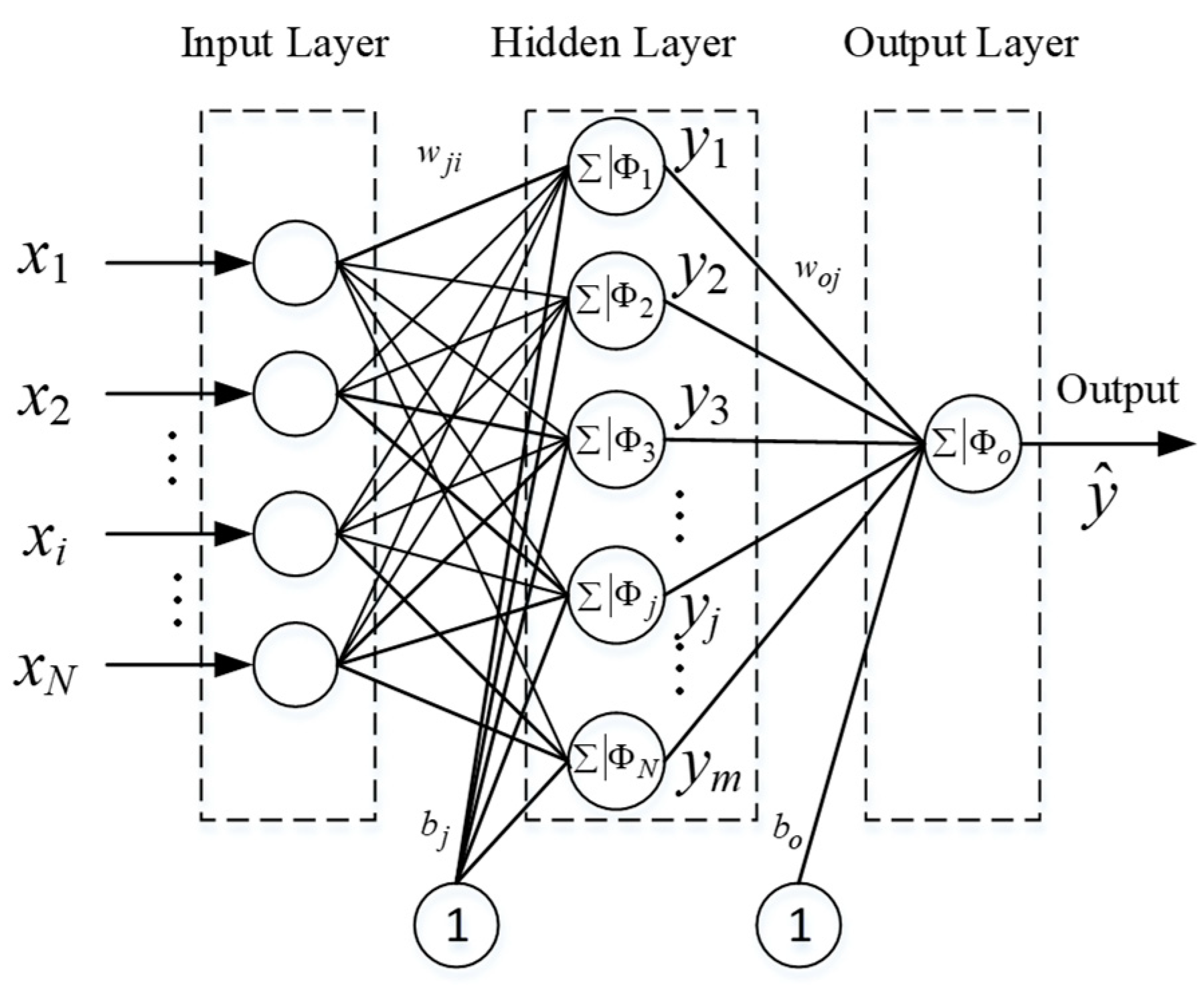
Multilayer perceptron (MLP) is a type of classical artificial neural network architecture. As shown in
Figure 1, MLP neural networks often contain one or more hidden layers between the input and output layers. The feedforward neural network was the first devised and the simplest type of neural network architecture, which contains multiple neurons defined in hidden layers. There are connections or edges between neurons from adjacent layers. All these connections have weights associated with them. Feedforward means that the data flows from the input layer to the output layer in just one direction (forward). The MLP trained with the back-propagation learning algorithm is named as back-propagation (BP) neural network, where the feedback data from the output layer is applied for weights optimization.
In a BP neural network, a neuron is the basic computation unit. It receives inputs from external sources and/or other neurons in previous layers and generates one output. Each input is assigned one weight
, which is calculated based on its relative importance to other inputs. An activation function is applied to the weighted sum of its inputs in each neuron. The output of the hidden neuron
in a hidden layer can be expressed as:
where,
is the neural network input vector,
denotes the weight vector between the hidden neuron
and the inputs
,
is the bias, and
is the activation function, which is usually defined as a nonlinear function (e.g., a sigmoid function). Then, the output of the neural network can be expressed as [
23,
24]:
where,
is the activation function of the output neuron, which is normally taken as a linear function,
is the final output of the MLP network,
is the bias value of the output neuron
, and
is the synaptic weight value from the hidden neuron
to the output neuron
.
The back-propagation algorithm is the most widely applied algorithm for training MLP neural networks. It works with the training data, so it is a kind of supervised training approach. During initialization, all the weights are initialized randomly. For each input from the training dataset, the ANN is triggered and provide one output. This calculated neural network output is compared with the objective output provided within the training data, yielding the residual error, and is called the cost function. The partial derivatives of the cost function for corresponding parameters are propagated back through the back-propagation process. Then, any gradient-based optimization algorithm can be applied to update the network weights. Repeat this process until the neural network satisfies the given stopping criterion [
24].
The Levenberg-Marquardt algorithm applied in this study is a back-propagation algorithm, also known as the damped-least-square method. It is the fastest computationally efficient method for medium-sized feedforward neural networks. This algorithm is specifically developed to handle cost functions in the form of the sum of squared errors. It is not necessary to compute an accurate Hessian matrix.
The neural network weights updated by the Levenberg-Marquardt algorithm can be expressed as [
25]:
where,
is the index of iteration,
is the weight vector of the
training iteration as defined in Equation (4),
is the identity matrix,
is the step size, and
is the error value of the
training iteration between the outputs and targets.
where,
Z is the number of weights
and
P is the number of input samples.
is a Jacobian matrix of the
training iteration as defined in Equation (6):
2.2. Group Method of Data Handling Network
GMDH [
26] is an approach that involves growing a neural network, which has a self-organized structure. GMDH networks gradually increase the number of neurons (or partial models) and obtain a model structure with optimal complexity. Thus, this process avoids the large amount of work in network architecture selection.
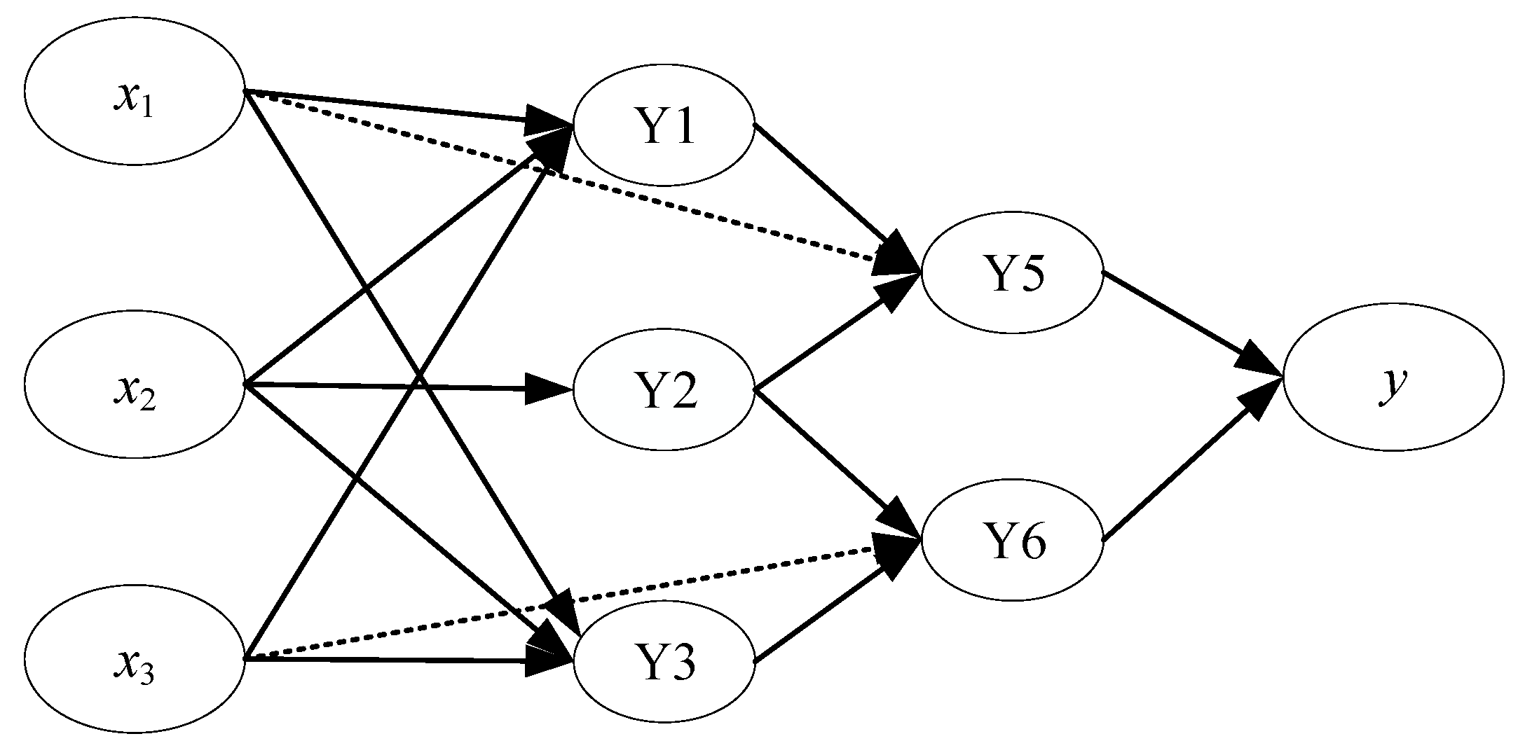
Figure 2 shows the structure of an example GMDH network with three inputs and one output. GMDH is a smart type of regression, which utilizes three steps to reach the final output (representation, selection, and stopping). The procedure can produce a high degree of polynomials in effective predictor.
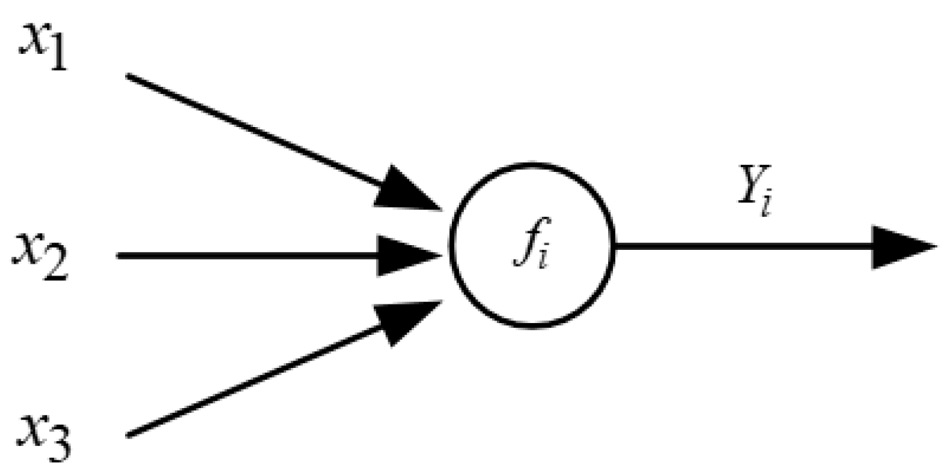
Figure 3 illustrates a typical computational node of the GMDH network with three inputs as an example [
27].
General connection between node inputs and output variables can be expressed by a complicated discrete form of the Volterra functional series (also known as the Kolmogorov–Gabor polynomial) in the form of [
28]:
where,
is the number of input variables,
,
, and
are inputs,
is the corresponding node output value, and
,
, and
are polynomials coefficients.
By means of the GMDH algorithm, a model can be represented as a set of neurons in which different pairs of them in each layer are connected through a quadratic polynomial and thus produce new neurons in the next layer. Such representation can be used in modeling to map inputs to outputs. The formal definition of the identification problem is to find a function,
, so that it can be approximately used instead of actual one,
, in order to predict output,
, for a given input vector,
, as close as possible to its actual output,
. Therefore, the output of the GMDH network for signal output can be written as [
28]:
In this way, such a partial quadratic description is recursively used in a network of connected neurons to build the general mathematical relation of inputs and output variables given in Equation (8). The coefficient is calculated using regression techniques in a least-squares sense so that the difference between actual output, , and the calculated, , for each pair of , , and as input variables are minimized.
The critical step is to determine a GMDH neural network by the root mean square error (RMSE), so that the square of squared differences between the actual output and the predicted one is minimized, that is:
where,
N indicates the number of data samples.
The main procedure for GMDH implementation can be summarized in the following steps:
- Step 1.
Divide data sample into training and validation sets. The training data was used for estimating the weights of neurons and the validation data was used for organizing the network architectures.
- Step 2.
Determine all neurons (polynomial descriptions) that consisted of all the possible combinations with three inputs among all the input variables. Then, estimate the coefficients of polynomials with the training data set.
- Step 3.
After training the first layer, select the best-fitting neurons via the validation data using the RMSE selection criterion.
- Step 4.
Check whether the termination condition was fulfilled (the current layer remained and only one neuron or the introduction of new neurons did not improve the overall performance of the network); if YES then STOP, otherwise the output of Step 2 was applied as the inputs for the next layer, and proceed to Step 1.
- Step 5.
Finally, the terminating condition was satisfied, the final structure of the network was obtained. To obtain the final model, the path of the neurons that corresponded to the lowest criterion was tracked back in each layer.
The GMDH network can be viewed as a polynomial neural network, where the node function was a polynomial rather than a sigmoid function. The parameter optimization was based on the least-square-fitting algorithm rather than iterative algorithm of BP neural network. Therefore, training in the GMDH network did not need a large amount of time. Moreover, the GMDH network did not have the problem of over-fitting, which was a difficulty in artificial neural networks.
This paper provided a novel framework based on the GMDH network for condition monitoring within the wind turbine paradigm, compared the GMDH condition monitoring model accuracy considering different input parameters combination for input parameter selection, and made a comparison with BP NN based condition monitoring to evaluate its performance.
3. Case Study
In this paper, the supervisory control and data acquisition SCADA data was collected from a wind farm located in China, which consisted of 121 parameters [
15]. Condition monitoring based on temperature signal was one of the most common methods in wind turbines using the SCADA data. According to previous research [
15], ambient temperature, wind speed, and power output were the most related parameters to gearbox oil temperature that could indicate the gearbox health condition. In terms of the data sampling rate, it was usually recorded at 5 min intervals, which aimed to reduce operational data collected from wind turbines. A 2.5 MW wind turbine equipped with the doubly fed induction generator was selected in this paper.
3.1. Parameter Selection for GMDH
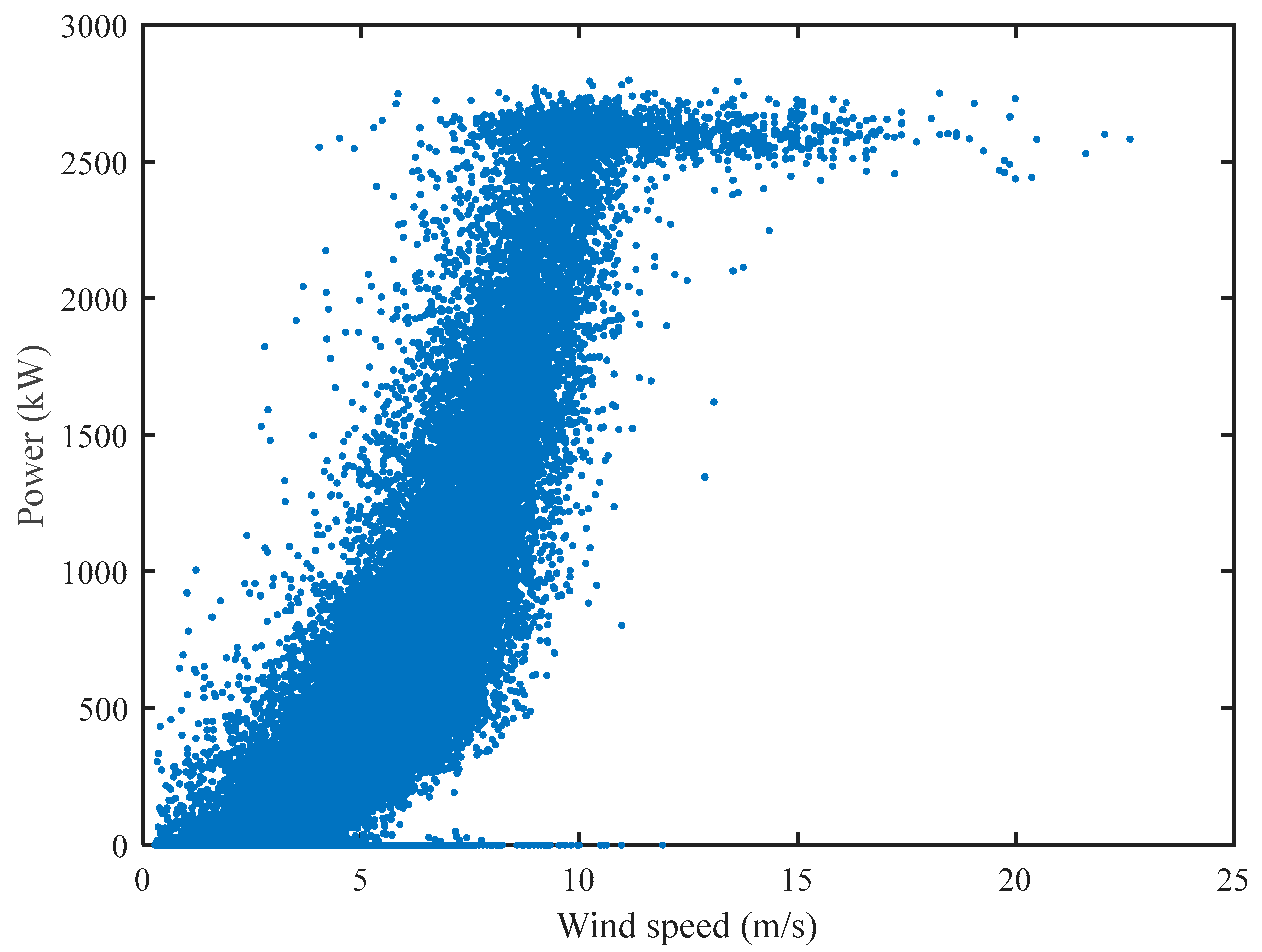
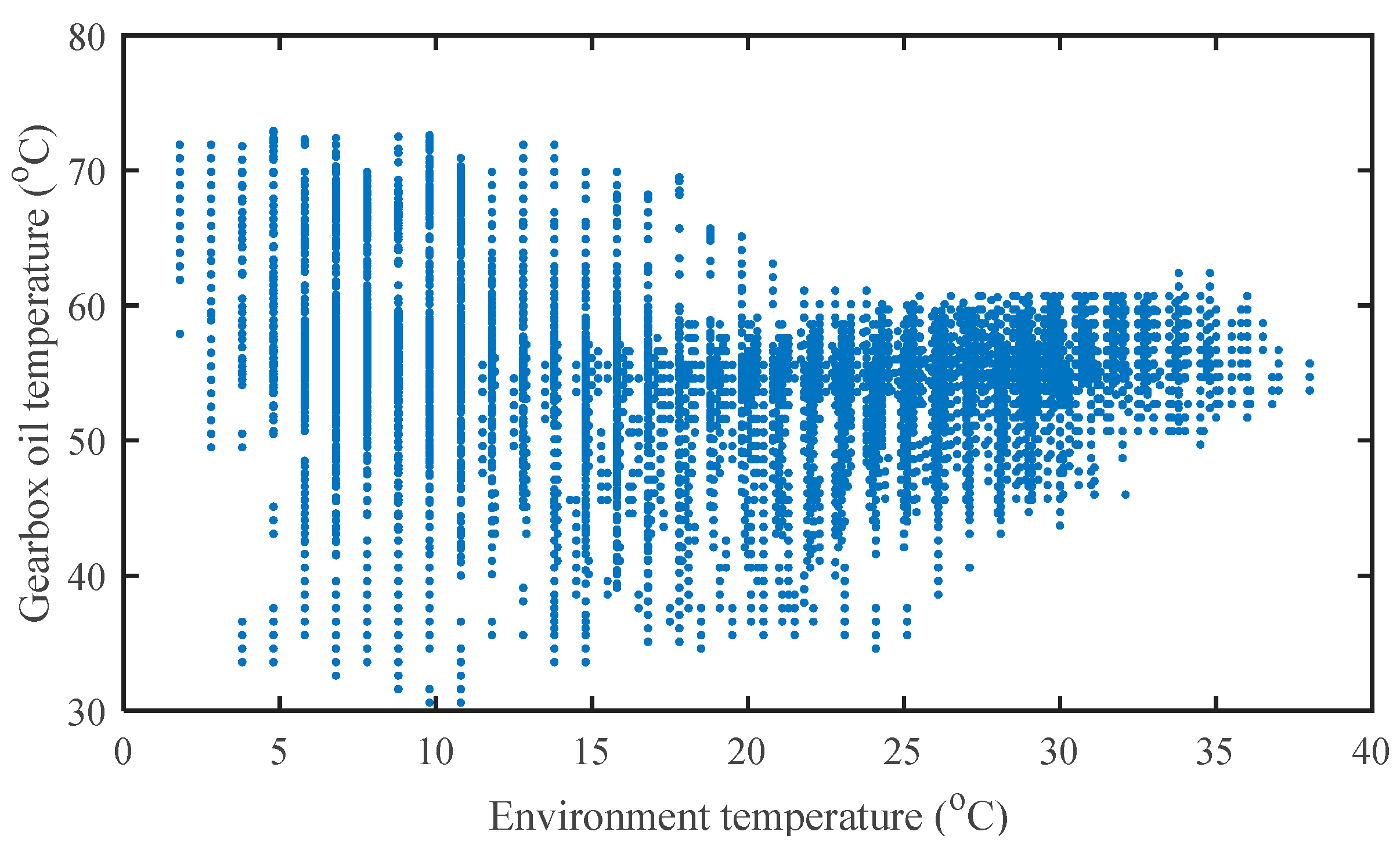
Figure 4 shows the power curve of a 2.5 MW wind turbine. The power output of the wind turbine varied with the cube when the wind speed was less than the rated wind speed of 10 m/s. When the wind speed was below 3 m/s, the torque from the wind turbine rotor was insufficient to allow generator operation. Meanwhile, the wind turbine was shut down to prevent the wind turbine from being damaged when the wind speed was larger than 20 m/s. When the wind speed was between the rated speed and the cut-out speed, the power output of the wind turbine was limited to the rated power (10 m/s to 20 m/s in this paper). The condition monitoring model accuracy was not only determined by the model parameters, but also by the input variables selection. For example, a key factor affecting heat dissipation in a transmission was air temperature. The relationship between the air temperature and the gearbox oil temperature is illustrated in
Figure 5. The heat dissipation of the gearbox was worse when the temperature was high than when the temperature was low. Hence, the gearbox temperature was able to change over a wide range in winter and over a small range during summer. It could be seen that both the power curve and the relationship between the air temperature and gearbox oil temperature were non-linear. Hence, the GMDH algorithm was suitable for wind turbine condition monitoring application.
In order to illustrate the impact of the parameter selection, a comparative analysis was performed, which contained wind speed with ambient temperature, wind speed with power output, power output with ambient temperature, and a combination of the above three input variables.
During the model training, the critical factors were selected manually by many trials. The main critical factors for the GMDH network applied in this research were as follows: 3 degree polynomials were applied in neurons in this research, maximal number of neurons in a layer was 6, and the criterion value was 0.005.
The gearbox oil temperature was selected as the wind turbine condition monitoring signal. Analysis results of the condition monitoring model considering different types of input variables are illustrated in
Table 1. The RMSE of the condition monitoring models considering three-input variables was less than two-input condition monitoring model, which reached 0.077 for the three-input condition monitoring model. The above results showed that the condition monitoring model with three-input variables was more accurate than condition monitoring model with two-input variables. Consequently, the condition monitoring models developed were based on the three-input variables in this paper.
3.2. CASE 1: Condition Monitoring Based on the Gearbox Oil Temperature
In this case study, the actual wind turbine data obtained from a wind turbine SCADA system had been compared with the corresponding condition monitoring prediction model output to calculate the residual signal. The GMDH neural network was applied to predict gearbox oil temperature to achieve the fault detection of wind turbine gearbox. The actual gearbox oil temperature data gained from the wind turbine SCADA data was compared to the GMDH condition monitoring model output, which aimed to detect the fault of gearbox fault. The SCADA data of air temperature, power output of the wind turbine, and wind speed from a healthy wind turbine was selected as the training dataset to calculate the parameters of GMDH condition monitoring prediction model. In order to validate the performance of GMDH based condition monitoring model, back propagation (BP) neural network was adopted to make comparisons with the proposed method.
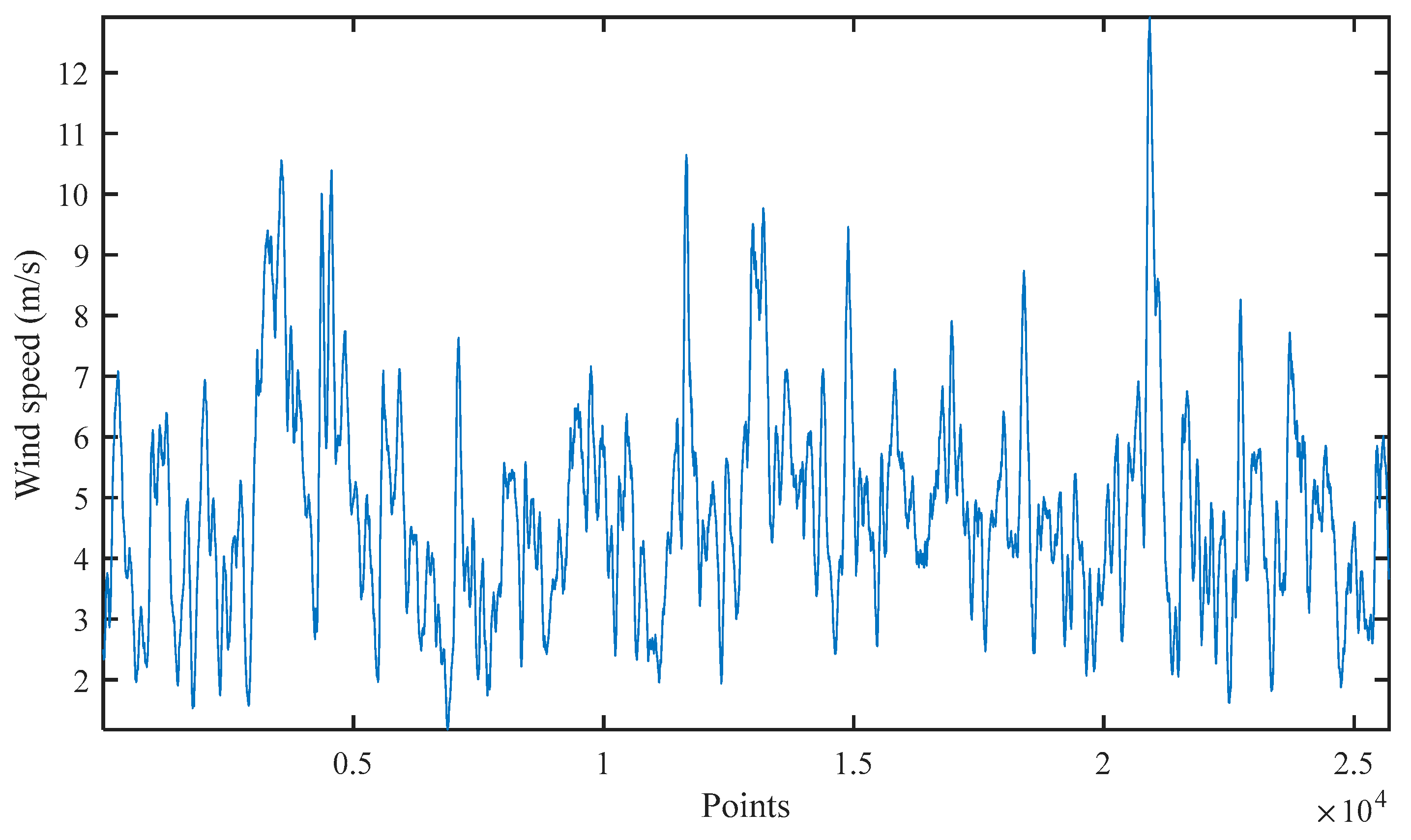
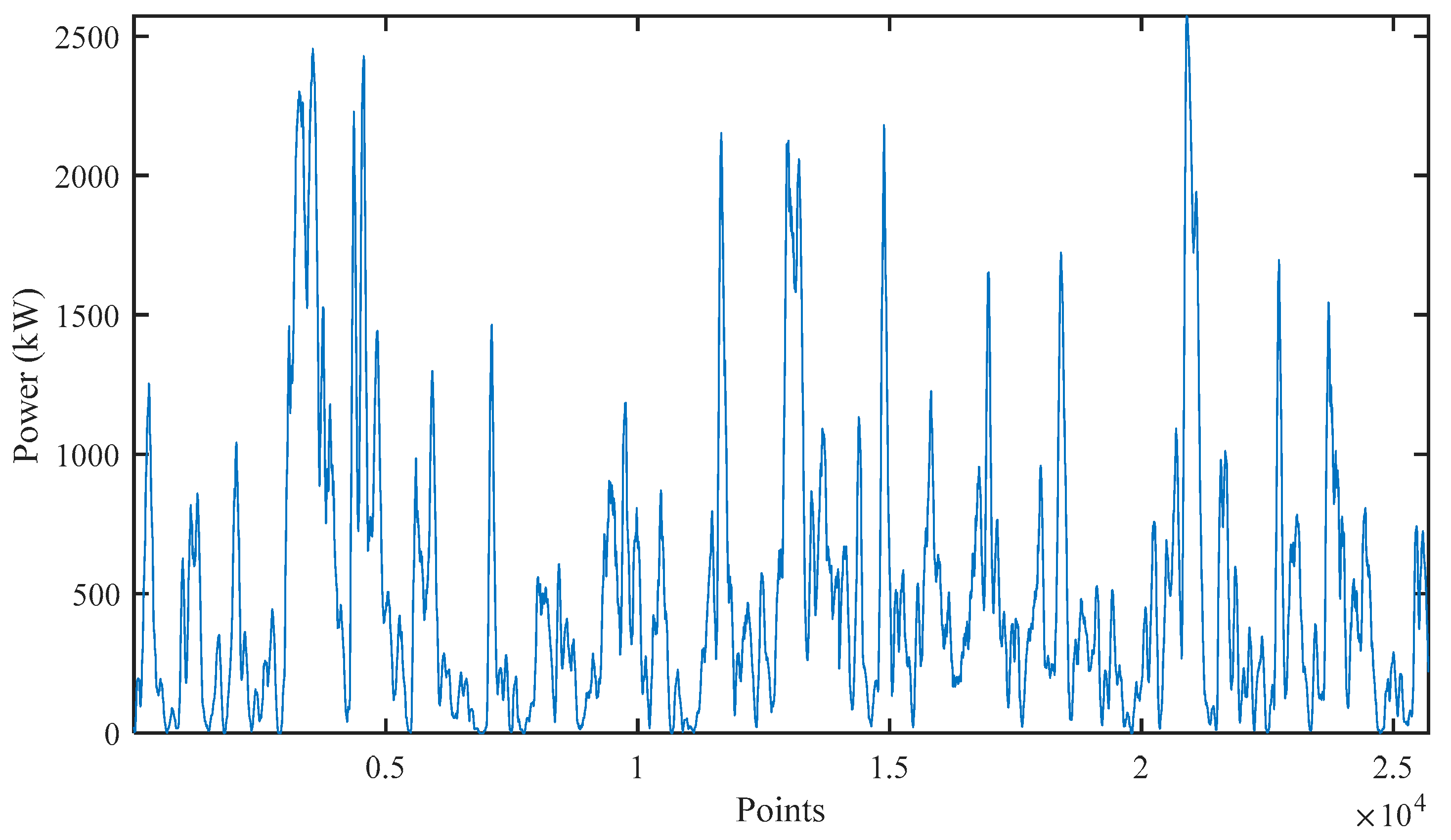
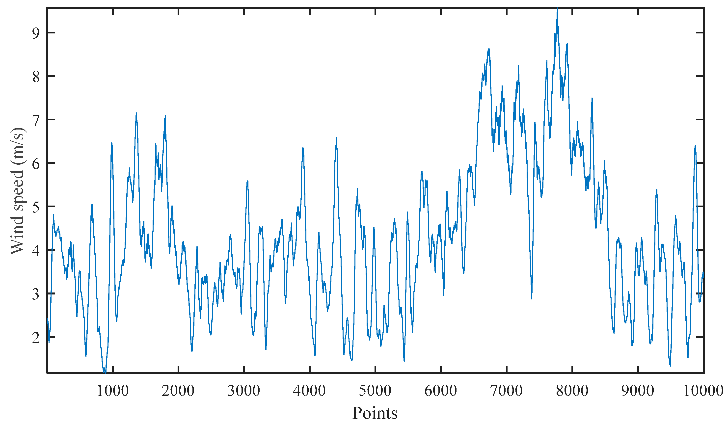
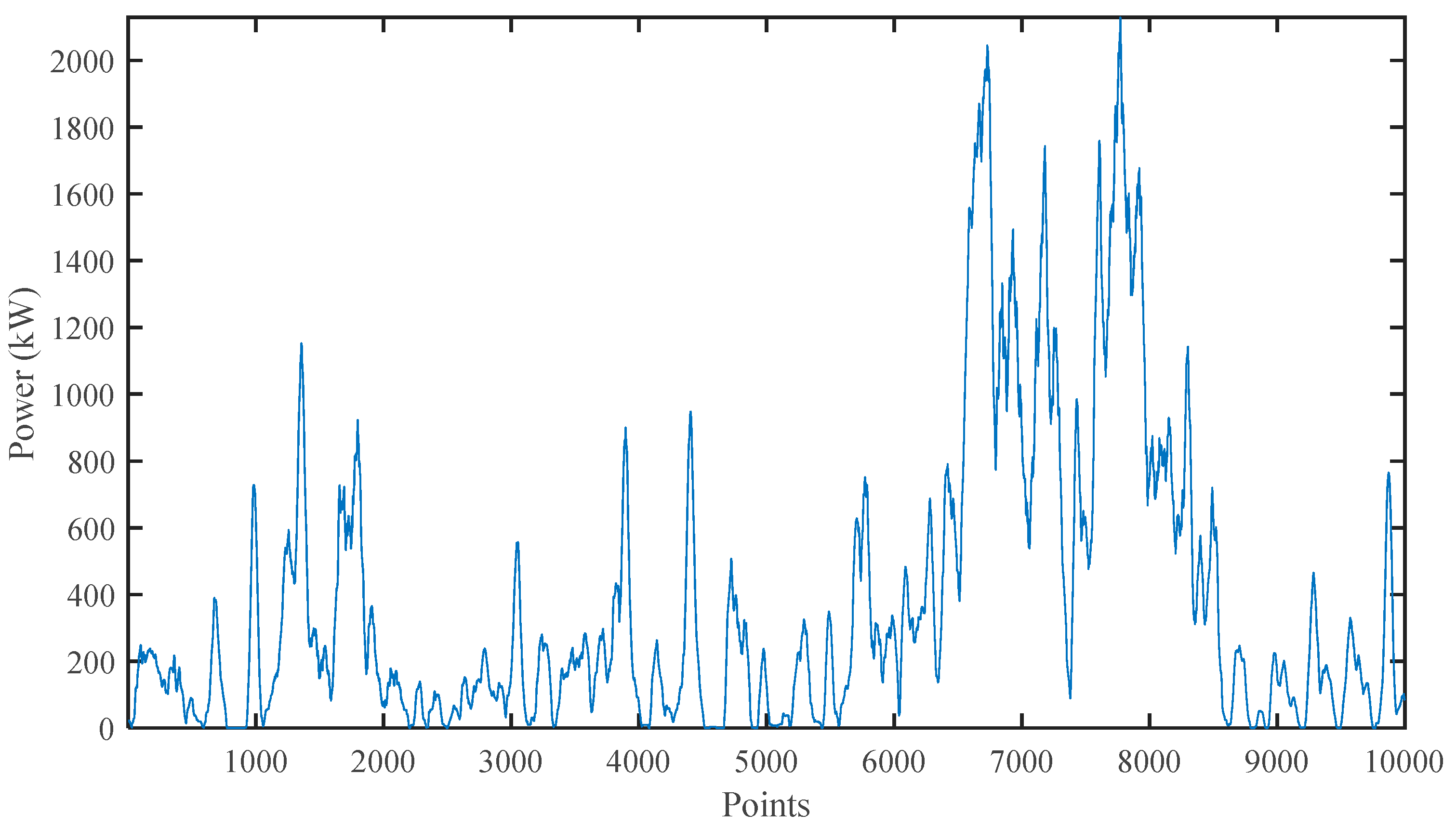
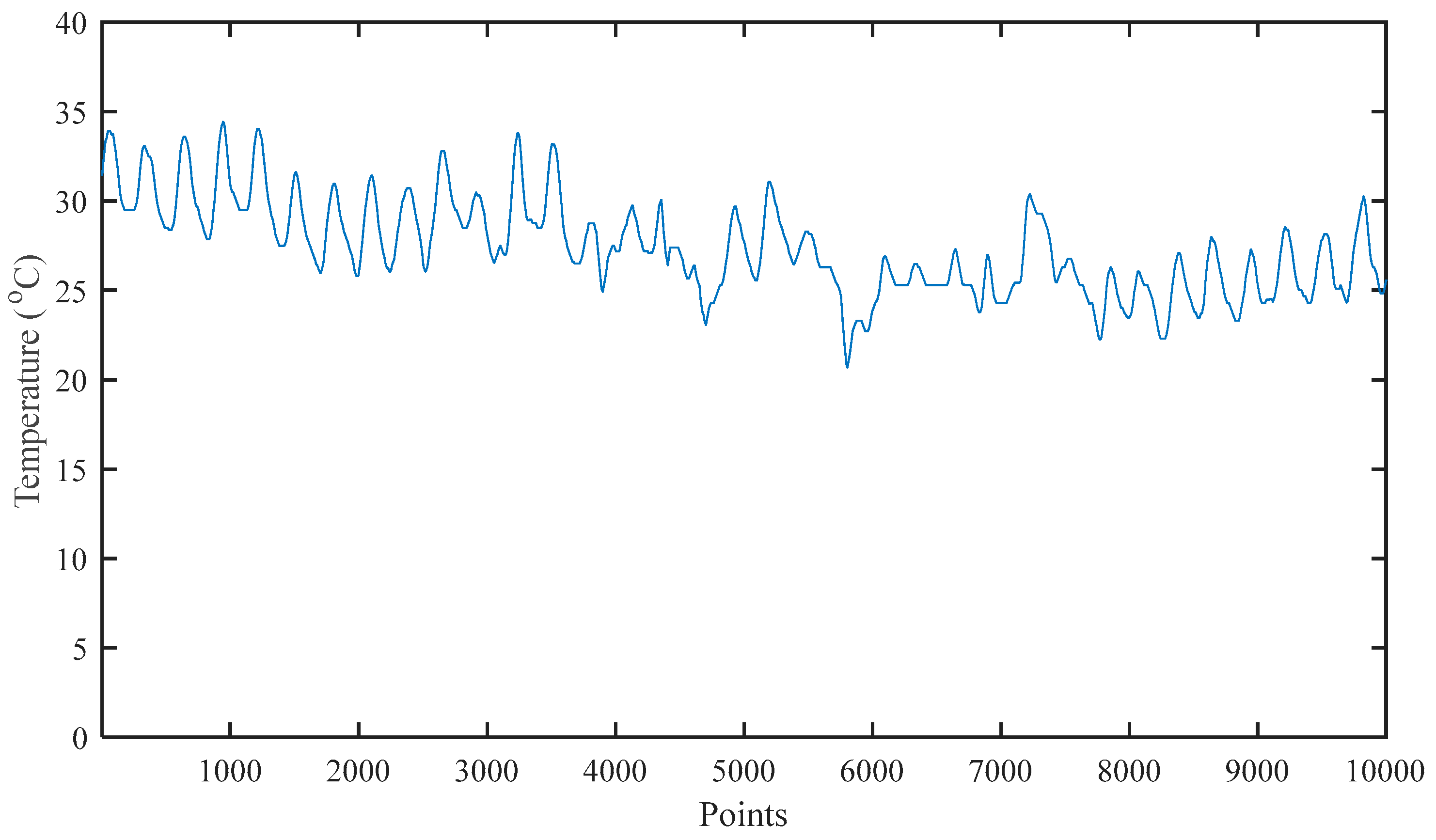
Figure 6 presents the wind speed of the wind farm obtained from the wind turbine SCADA system. The corresponding power generation of the wind turbine and actual ambient temperature are shown in
Figure 7 and
Figure 8, respectively.
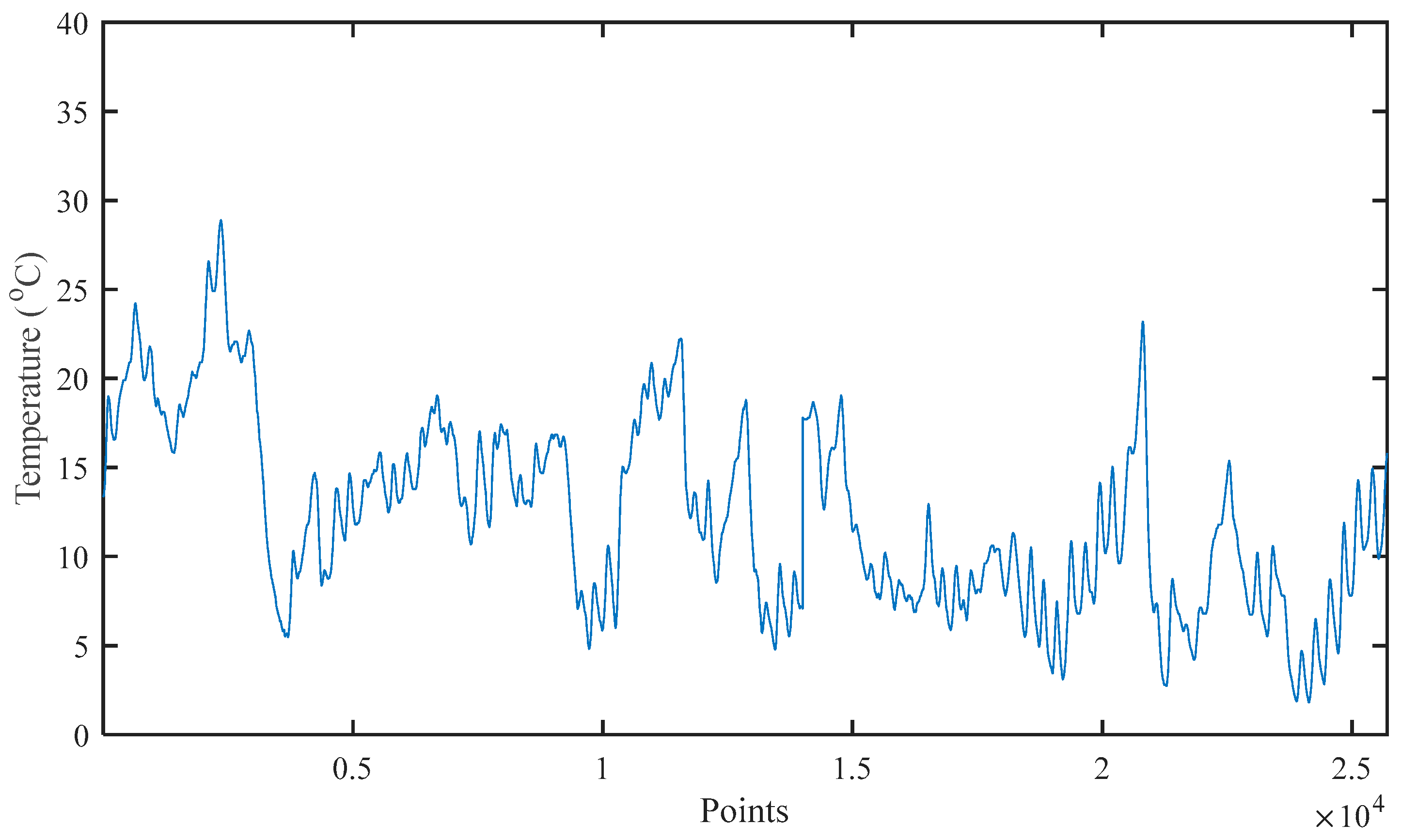
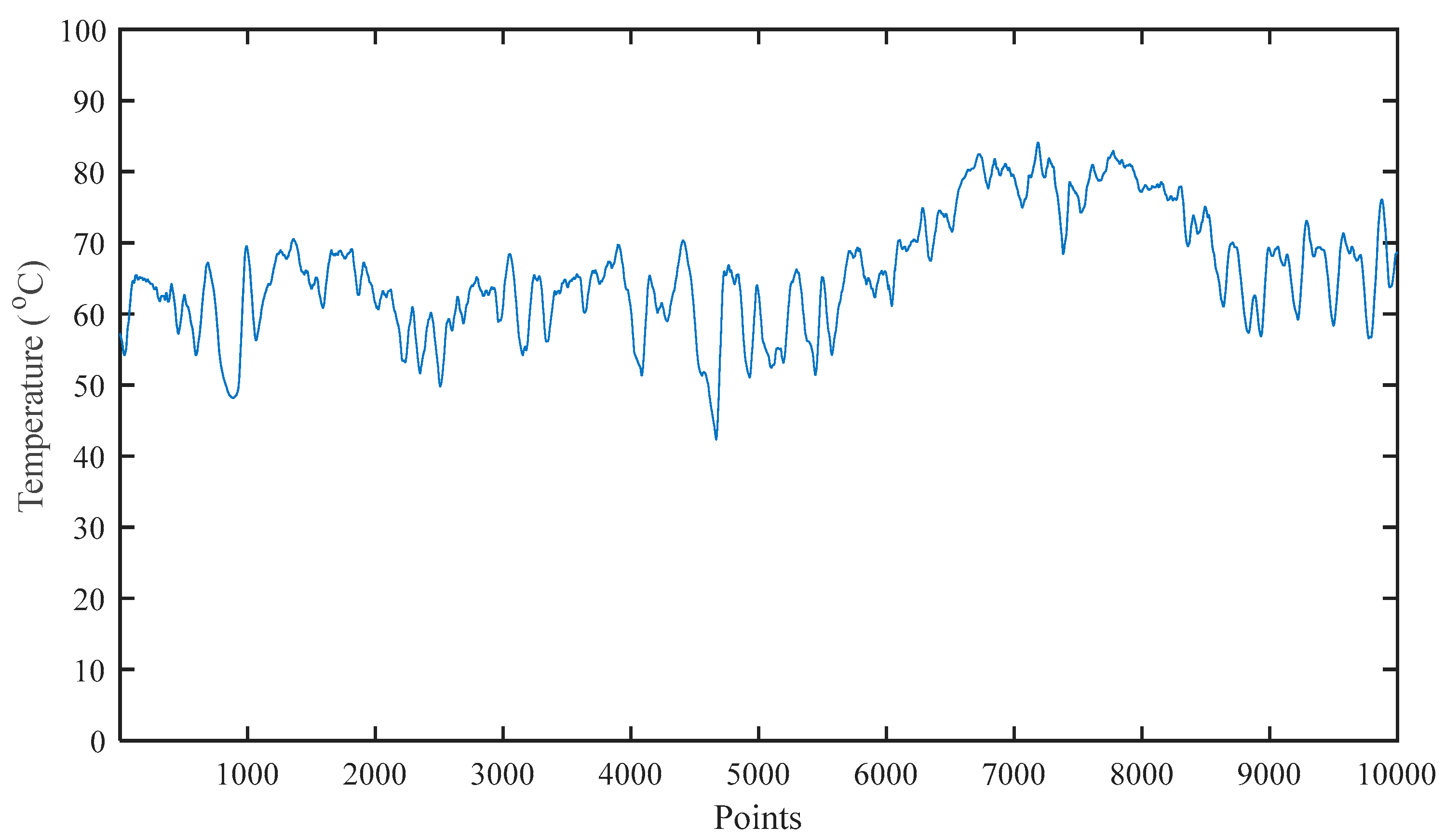
Figure 9 shows the actual temperature of wind turbine gearbox oil obtained from the SCADA system of a wind turbine with a gearbox fault.
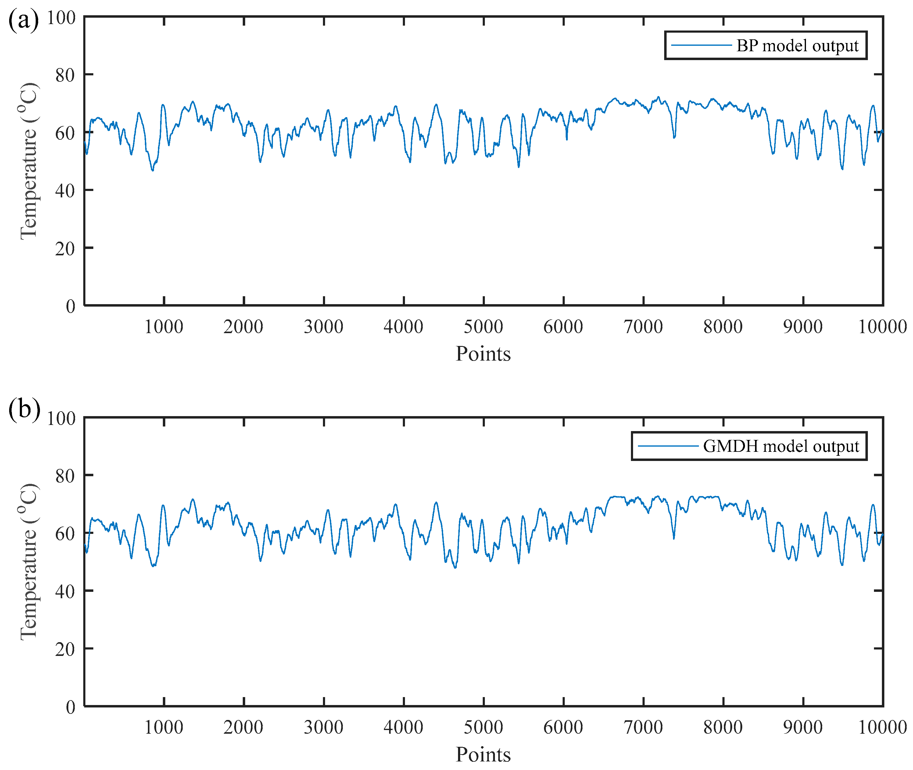
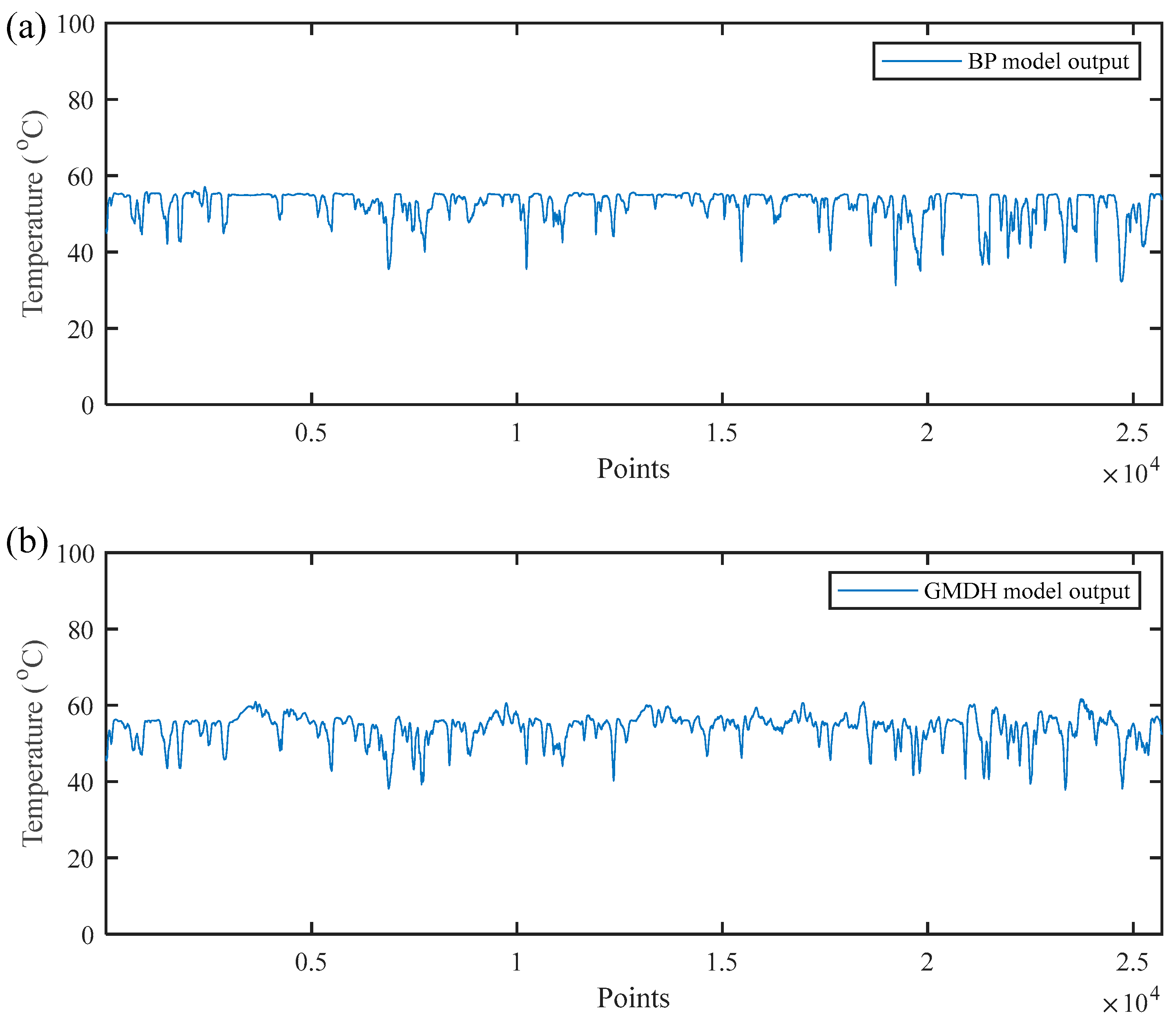
Figure 10 illustrates the condition monitoring model output of wind turbine gearbox oil temperature from a BP model and a GMDH model.
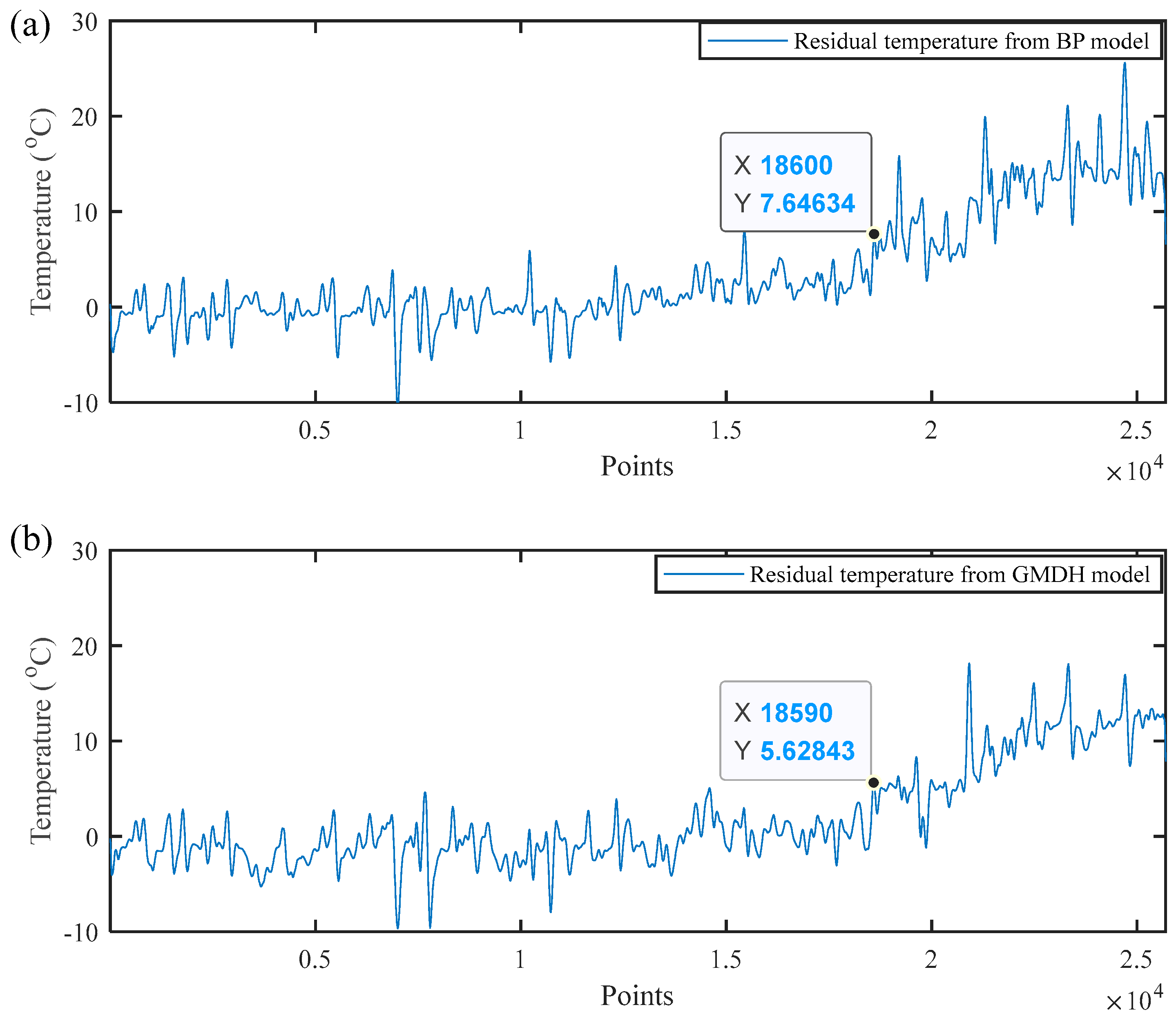
Figure 11 shows the residual gearbox oil temperature signals from the BP model and GMDH model. The residual signals were obtained from the difference between a condition monitoring model output and the actual wind turbine gearbox oil temperature from the SCADA data. It showed that the residual signal between the actual gearbox oil temperature of the wind turbine and condition monitoring model output stayed at a low level with fluctuations since the beginning and exhibited an increasing trend at the sampling point 18,600 for BP model and at sampling point 18,590 for GMDH model; thereafter, successive residual errors held at a high level, which indicated a potential fault occurred in the wind turbine gearbox. In order to verify the correctness of the proposed condition monitoring model, the alarm logs of the wind turbine SCADA system had been investigated to check this abnormal behavior which occurred in the wind turbine gearbox. The results showed that both the BP model and GMDH condition monitoring model outputs were consistent with the alarm logs of the wind turbine SCADA system. The fault detection results based on the GMDH condition monitoring model provided the abnormal indication slightly earlier than that of BP based model.
3.3. CASE 2: Condition Monitoring Based on the Generator Bearing Temperature
Case 1 validated the effectiveness of the GMDH network using the SCADA data with a gearbox fault. To further verify the proposed GMDH condition monitoring method, a wind turbine gearbox bearing fault was selected as the research object. The data applied for case study 2 were different than that for case study 1. They were two separate faults that occurred at different time periods.
Figure 12 presented the wind speed of the wind farm obtained from the wind turbine SCADA system. The corresponding power generation of the wind turbine and actual ambient temperature were shown in
Figure 13 and
Figure 14, respectively.
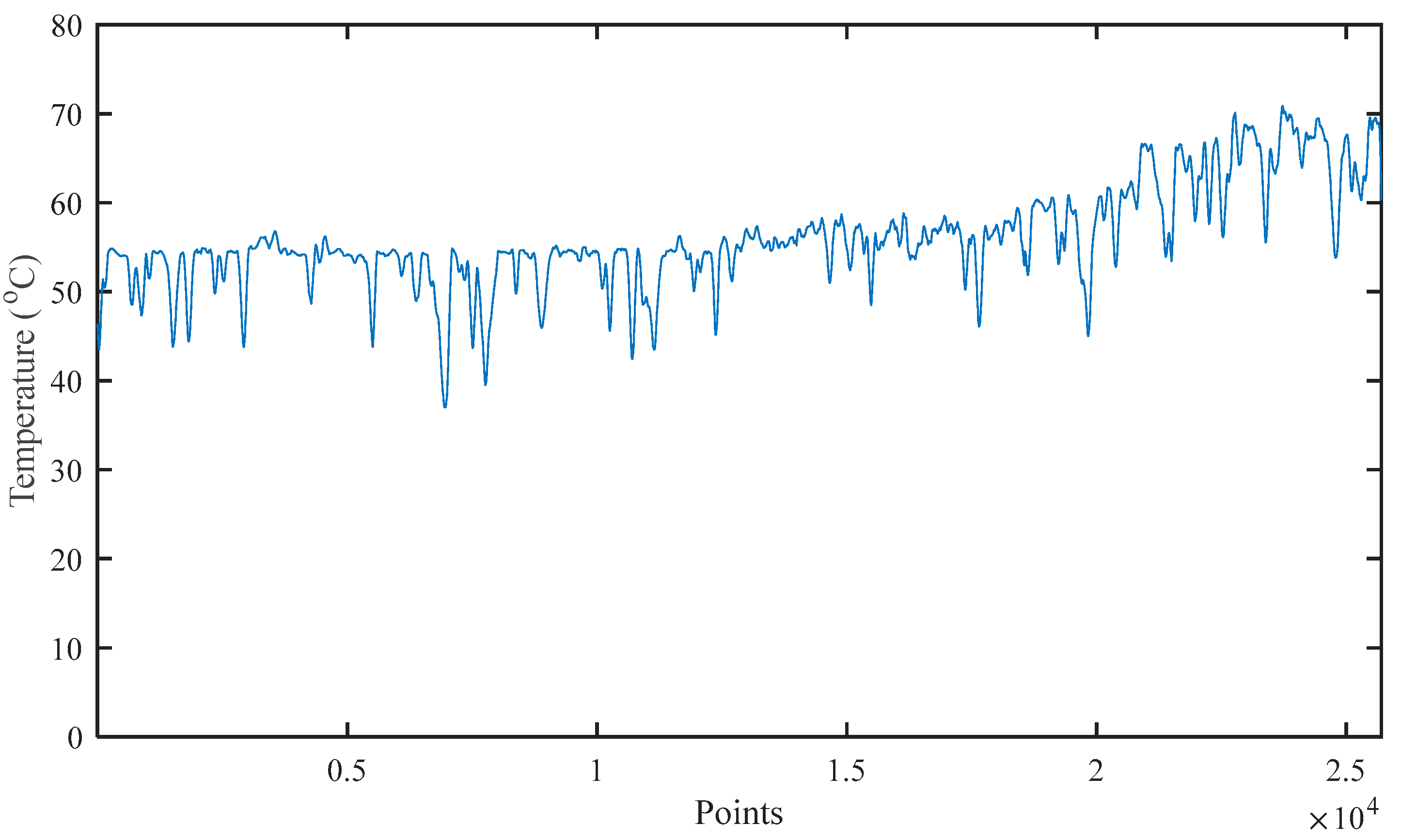
Figure 15 showed the actual temperature of the wind turbine gearbox bearing obtained from the SCADA system of a wind turbine with a bearing fault.
Figure 16 illustrated the condition monitoring model outputs of wind turbine gearbox bearing temperature from a BP model and a GMDH model.
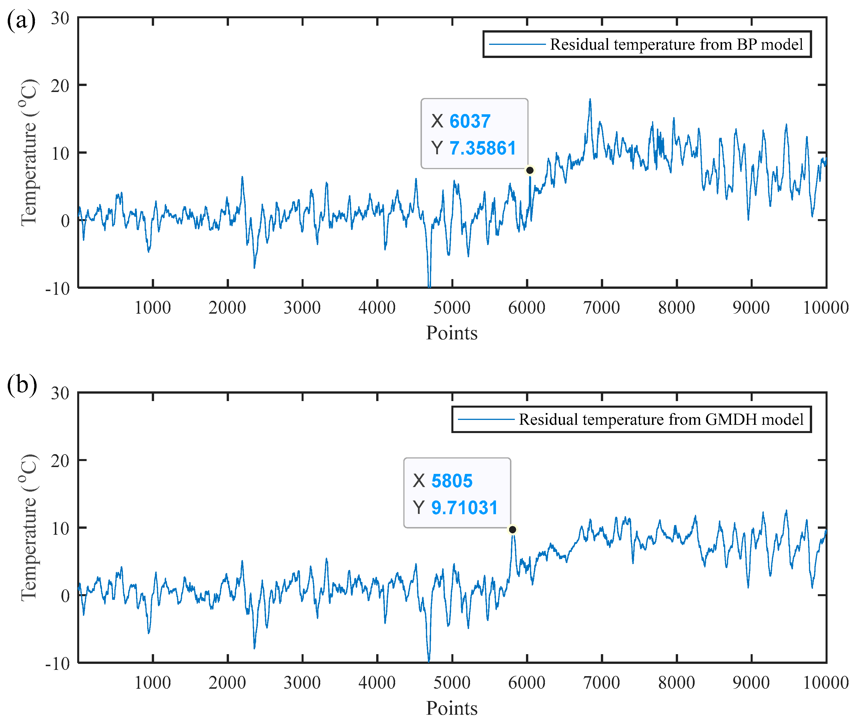
Figure 17 showed the gearbox bearing temperature residual signals, which were obtained from the difference between condition monitoring model output and the actual wind turbine gearbox bearing temperature for both models. It showed that the residual signal stayed at a low level with fluctuations since the beginning and exhibited an increasing trend at sampling point 6037 for the BP model and at a sampling point 5085 for the GMDH model; thereafter, successive residual errors held at a high level, which indicated a potential fault occurring in the wind turbine gearbox bearing. To verify the correctness of the proposed condition monitoring model, the alarm logs of the wind turbine SCADA system had been investigated to check this abnormal behavior occurred at the wind turbine gearbox bearing. The results showed that both BP and GMDH condition monitoring model outputs were consistent with the alarm logs of the wind turbine SCADA system. The fault detection result based on GMDH condition monitoring model provided the abnormal indication at 52 sampling points earlier than that of the BP based model. Furthermore, the increasing trend of residual temperature from the GMDH model was more significant than that from the BP model, which meant that the GMDH based model could provide an effective fault detection indication at the early stage of the gearbox bearing fault case.
Finally, a comparison of the calculation time between these methods is listed in
Table 2. It was obvious that the calculation time of the GMDH model was less than that of the BP model for both case studies, especially for case 2, which was 1/3 of the BP model. It showed that the GMDH model had greatly shortened the calculation time.
4. Conclusions
A novel wind turbine condition monitoring the approach based on GMDH neural network using SCADA data was, for the first time, proposed in this paper. In order to validate the effectiveness of the proposed method, the SCADA data collected from a commercial wind farm had been adopted. Two case studies had been carried out to illustrate the wind turbine condition monitoring by using gearbox oil temperature and gearbox bearing temperature. The results showed that the GMDH provided earlier and more significant fault indications than the traditional back-propagation neural network algorithm, while greatly shortening the calculation time. Moreover, GMDH was a kind of self-organized network, and the trained model was simple, easy to understand, and could avoid the over-fitting problems. Hence, the proposed method was suitable for real time implementation in condition monitoring systems, which could reduce condition monitoring cost, and in the meantime, increase the monitoring efficiency.


