Optimising Photovoltaic Farm Location Using a Capabilities Matrix and GIS

Abstract

Renewable energy sources provide an important solution in environmental protection activities and in the process of shaping sustainable development. The search for optimal locations enabling full exploitation of the energy intensity of real estate presents a significant challenge in terms of geoinformation analysis methods in a GIS environment. The aim of the study was to develop a capabilities matrix for the location of photovoltaic farms and, based on this, to compile a map of decision alternatives for these locations. The first stage involved the determination of the spatial features (stimulants and destimulants), which were significant in the context of photovoltaic (PV) farm location. During the analysis, the scope of the necessary data and their sources, which included topographic vector studies, aerial images, and the OpenStreetMap open data, were determined. The next stage was to determine the weights of the features which were significant in the context of photovoltaic (PV) farm location. To this end, the Multicriteria Decision Making (MCDM) method, including the Analytic Hierarchy Process (AHP) method, was employed. For the verification of the results, the entropy measure was also used. Entropy was calculated based on the diversity of previously identified geospatial features that shape the optimum conditions for their location, based on the photovoltaic farms already existing in Poland. A total of 555 photovoltaic farms were analysed. The next stage assumed the performance of geoinformation analyses using GIS tools and the development of a capabilities matrix for the PV farm location for the selected commune in Poland. The final stage involved the compilation of a PV decision alternative map for the selected commune based on the capabilities matrix. As a result, as an example, a ranking of plots was developed as decision-making alternatives for the municipality of Czarnia located in the northeastern part of Poland. It shows which parcels of land primarily have the dimension of spatial features that are favourable for the location of PV. More than 6900 parcels were analysed, in which 176 presented the highest value of the index of optimal PV location generated using the AHP method. This method provides a basis for further work by identifying optimal locations taking into account existing spatial conditions. The analyses carried out can be an important document in the future for spatial management, in particular for the location of new PV farms. As a continuation of the research, the authors will work on expanding the scope of the analyses and automating the entire process.

1. Introduction

Due to the increasing air pollution and global warming, renewable energy sources, e.g., photovoltaics, are used to produce electricity, thus mitigating the effects of climate change and promoting sustainable development. An increasing number of photovoltaic farms are emerging. Their viability is determined by many factors arising from both natural and anthropogenic determinants [1,2]. Due to the multiplicity of these factors (spatial features) and their heterogenicity in various parts of the world, the determination of the optimum location of a photovoltaic (PV) farm is not easy.

The literature on the subject provides many different approaches to the subject of making a decision on the location of investment projects, e.g., photovoltaic farms. What unites all the studies, in principle, is the research based on an analysis of spatial features, which either favour or include the location of investment projects of this type (stimulants and destimulants) [1,3].

Many studies searching for the optimum PV farm location have been conducted by the Multicriteria Decision Making (MCDM) method [4,5,6]. The MCDM approach is a broad group of methods for assessing multiple, often conflicting, criteria in order to make a decision [4,7,8]. The MCDM, in combination with GIS systems, is very widely used in the analysis of renewable energy factors [9,10,11], including the identification of renewable energy sources [12,13,14,15,16] or the determination of the technical potential of this energy [17,18,19], and the planning of the location of power plants using renewable energy sources [5,20,21,22]. Pokonieczny applied GIS modelling in combination with neural network theory to locate wind farms [23]. GIS analyses use both vector and raster data concerning physical aspects of the Earth’s surface, which model the spatial features, but in addition also use satellite data to derive land use/land cover maps (e.g., from SPOT-4) or a Digital Elevation Model (DEM) (e.g., from Shuttle Radar Topography Mission (SRTM)) [24]. Mokarram et al. used the MCDM method in combination with the Dempster–Shafer theory with a fuzzy system to identify the optimum solar farm sites in the Fars province (Iran). The authors used the probabilistic uncertainty model to determine the uncertainty of the decision system and, consequently, proposed suitability maps with desired confidence levels [5].

The application of the MCDM method in geospatial analysis, using GIS technology to determine the location of the PV farm, aims to determine the weight of the criteria (spatial characteristics) that generate such location and compile maps of decision alternatives. It is important, in these activities, to properly identify the spatial features (stimulants) which make the particular location optimal. It is, therefore, necessary to analyse the target space, which, due to its natural (e.g., the climatic location, terrain) and anthropogenic determinants (e.g., the distance from the essential spatial infrastructure or a lack of destimulants), can generate this potential very differently [25]. An example can be found in a study by Alavipoor et al. [26], which, in order to determine the PV farm location, took into account the spatial features arising from the climatic and topographic conditions, such as the relative air humidity or dust and the topography, e.g., the inclination and height. Other studies [27] additionally mention a distance from roads and water resources or residential areas [1]. Siefi et al., however, did not take the climatic factors into account. On the other hand, according to Tahri et al. [11], these factors are among the most important ones in the context of PV farm location. In certain countries, an important element of the analysis is the elimination of inappropriate locations for safety reasons [28]. Boeber et al. [29] divide the criteria that are of significance when determining the PV farm location into two groups: environmental (which includes the terrain slope, solar radiation, soil quality class, and the existence of protected areas) and economic (which includes the distance from roads, medium voltage grids, and the minimum continuous surface). Mierzwiak and Calka, however, added a third group of criteria, i.e., technical criteria [30]. It should be stressed that the significance of certain features of the space arises from the determinants and legal provisions of individual countries [29].

The aim of the current study was to analyse the features in an aggregate way in relation to the above-mentioned publications. Under the assumptions made, based on the literature on the subject, the authors decided to analyse 17 features, grouping them into three categories (classes): environmental, climatic, and anthropogenic. The conducted analyses showed that the proper identification of a set of spatial features either favouring (stimulants) or preventing (destimulants) the establishment of a PV farm is a difficult task. Thus, the paper presented here is an attempt at a methodological approach to the assessment of the space in terms of the investment project type under consideration. Another important element of the issue addressed is the fact that Poland is located in a warm temperate transitional climate that is characterised by high variability of weather conditions throughout the year.

The observation of the inventoried photovoltaic farms in the country enabled the authors to formulate the basic thesis that assumes the existence of spatial features that favour the location of the above-mentioned investment projects as part of the renewable energy source. An important intermediate goal of the study was to objectify the datasets and the sources of their origin, regardless of the spatial scale of the feature. The identification and appropriate assessment of the features, conducted at a further stage, will enable the identification of the optimum farm location (decision alternative).

The authors are aware that a statement that a certain configuration of the features of a particular space is more “friendly” to an investment project, i.e., a photovoltaic farm, does not mean that it will certainly occur in a particular location. However, based on the empirical research carried out, it should be concluded that the probability of selecting an appropriate location using this method is considerably higher.

The suggested methodology serves the purpose of identifying the places with the greatest potential for PV, but is just a first assessment, requiring a later study with higher spatial detail and more reliable data.

2. Geoinformation Analysis in Decision Making

The main elements of a multi-criteria geoinformation analysis supporting decision-making processes include decision makers, the criteria, and decision alternatives. The aim of such an analysis is to achieve the desirable state, answer the questions asked as a result of the spatial data analysis, and achieve new, reliable spatial information. A decision maker is an individual (or, possibly, a group of individuals) responsible for making a decision based on the developed decision alternatives, which, in turn, are derived from the criteria established [31]. The criterion includes the concept of both the objective and the attribute. The attribute should be understood here as a feature of a geographical object or a relationship between objects which can be measured at a selected measurements scale, e.g., quantitative, qualitative, or rank, and which has a clearly defined spatial location. In light of the above, the aim of this geoinformation analysis is to identify the desirable state of the system under consideration in the context of the optimum photovoltaic farm location.

Spatial decision alternatives referring to the geographical space can be developed for the purposes of the selection of [31,32]:

-

of the action—i.e., an answer to the question: what would need to be done?

-

and the location—where would it need to be done?

Decision alternatives can be in vector or raster data format. A decision alternative in vector format can be represented by a point, a line, a surface, or a complex vector object, e.g., a network or a set/array of objects. The values of the criteria, i.e., the attribute values, are contained in a table and relate to spatial relationships (e.g., location or geometry), but can also be the result of additional spatial analyses. The values of the selected criteria can be expressed at different measurement scales and in different units. The vector data model is used when modelling discrete objects with precise contours and shapes. In contrast, a decision alternative in raster format is most often represented by the cells of a single raster, which have a specific size and position determined, for example, by the centre of the cell [31]. Each raster cell has an associated value, which can be defined by continuous or discrete values. This type of data is particularly used when modelling continuous objects with imprecise contours as well as optical and remote sensing data. This paper assumes the development of decision alternatives for the purposes of the selection of the site for an investment project, i.e., a photovoltaic farm.

The initial stages of a geoinformation analysis often require the definition of specific conditions affecting the development of decision alternatives, which may arise from legislation or rigid assumptions for the implementation of a project. An example could be the assumption that photovoltaic farms cannot be located in an area where a specific form of nature protection (e.g., a national park) is in force or where there is no possibility for a medium voltage connection within a radius of 200 metres. Due to the barriers arising from selected assumptions or other provisions, the decision alternatives can be divided into acceptable and unacceptable ones. A simple example of going through the process of criteria analysis and acceptable alternative development is shown in Figure 1.

The above example represents a situation in which both criteria must be satisfied in the primary field of assessment so that an acceptable alternative can be found. Therefore, to summarise: in order to develop an acceptable alternative in this case, in a particular area (the primary field of assessment), two criteria (spatial features) must be satisfied, i.e., must emerge in the space at specific values (a_i1 ≤ 200 and a_i2 ≥ IV).

2.1. PV Farm Location Criteria and the AHP Method

The determination of the criteria and their weights that are significant in the context of the optimisation of the location of a project is a fundamental and essential matter, as it determines the successful operation of the particular investment project [33]. By definition, the weight of a criterion is the value assigned to an evaluation criterion, which determines its relative significance in relation to other criteria under consideration [31] (p. 41). There are many methods for determining the weights of criterion significance [34,35,36].

According to the theory, the weights of w_j (where j = 1,2, …, n) should satisfy three basic assumptions [31,35]. Namely:

• The sum of the weights should amount to 1, i.e.,:

  $${\displaystyle \sum }_{j=1}^n{w}_j=1$$

  (1)
• The range of weight values should be from 0 to 1:

  $$0\le w_j\le 1$$

  (2)
• The weight values should be expressed on a quotient measurement scale. Therefore, the weight values indicate how many times one criterion is more important than another.

Where multi-criteria analyses are used in Geographic Information Systems (GIS), Malczewski and Jaroszewicz [31] (p. 44) propose the division of the methods for determining the criterion significance weights into two groups: local and global.

The local methods are a group of methods which assume that the criterion significance weight values are variable in the geographical space [31]. These methods include the method for determining the weights of the criteria aligned by the proximity relation. This method assumes the modification of preferences based on spatial relationships occurring between alternatives or between an alternative and certain locations that represent a spatial reference. The alignment in question involves two approaches:

-

after aggregating the criterion values to the alternative assessment value;

-

before aggregating the criterion values to the alternative assessment value.

These issues are described in detail by Rinner and Heppleston [37], Malczewski and Jaroszewicz [31], or Ligmann-Zielińska and Jankowski [38].

The global methods include the ranking method, index methods, the weight slider technique, the entropy-based criterion significance weight method, or the paired comparison method (PCM) [31,39].

The ranking method is mentioned as the simplest method used to determine the criterion significance weights [31]. According to this method, the criteria are ranked by their importance by assigning them numbers which are not yet weights. This is only a ranking scale. In order to carry out further analyses, the ranking developed in such a manner should be converted into a quotient scale in order to be able to carry out mathematical calculations. To this end, either the rank sum method or the rank inverse method can be applied [40,41,42].

The index methods include the coefficient estimation method and the point award method. The index methods are based on the decision maker’s estimation of weights according to the adopted scale, e.g., from 1 to 10, where 10 represents the most significant criterion, and the values are expressed on a quotient scale. Examples are described by, e.g., Malczewski and Jaroszewicz [31] and Hobbs and Meier [35].

The weight slider technique was described by Bodily [43] and involves an approach in which the decision maker compares the significance of a range of changes—from the poorest to the best values of a particular criterion, with the analogous changes in the values of the remaining criteria.

In the entropy-based criterion significance weight method, these weights are determined based on the values of individual criteria. In this case, it is assumed that the criterion weights can be determined based on the volume of information contained in a specific criterion and expressed by the entropy value. This method is based on the information entropy theory described by Shannon [44], where entropy is a measure of the volume of information in a message. Accordingly, each criterion can have its own significance weight, which indicates its effectiveness in the selection of a decision alternative. Kowalczyk used entropy to determine the quantity of information for the purpose of analysis and spatial planning of rural areas and to predict the directions of settlements around cities by analysing the entropy of built-up areas and determining the quantity of information [45]. In this study, the entropy measure was used to verify the significance of the features determined using the AHP (Section 2.2).

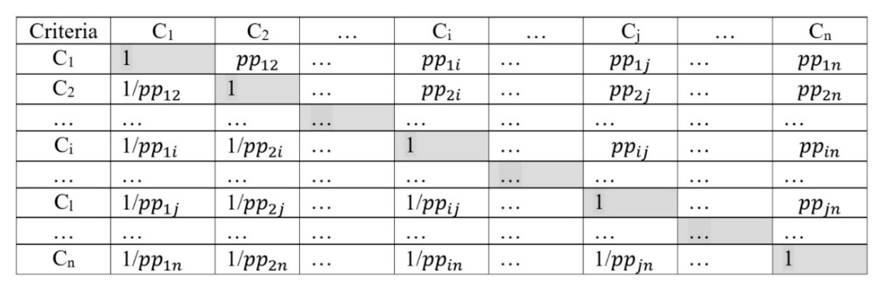
The paired comparison method (PCM) is an important part of the Analytical Hierarchy Process method [46,47] (AHP), as it is used to determine the weights of criterion significance. The PCM involves the development of a square matrix in which the criteria are compared against each other, i.e., in pairs. This yields a numerical representation of the relationship between two criteria related to a single, common objective. The paired comparison matrix has the following form [39]:

$$\left[\begin{array}{cccc}1& p{p}_{12}& \dots & p_{1n}\\ 1/p{p}_{12}& 1& ⋮& p_{2n}\\ ⋮& ⋮& \ddots & ⋮\\ 1/p{p}_{1n}& 1/p{p}_{2n}& \cdots & 1\end{array}\right]=\mathrm{PCM}$$

(3)

Which means that (Figure 2):

Where, for example, $p{p}_{il}$ should be interpreted as an assessment of the paired comparison of the i-th criterion (from the left side) with the l-th criterion (from the top). The values of the cells which are found under the matrix diagonal are, as can be seen in Figure 2, the inverse of the value above the diagonal. The judgment that will be made and indicate the dominance of any of the criteria compared against the objective can be described by Saaty’s universal reciprocal relationship scale [47] (

Table 1. Saaty’s universal comparison scale.

Significance Scale	Description of the Criteria Relation (Cn)
1	Equivalent (same preferred)
2	Equivalent to slightly preferred
3	Slightly preferred
4	Slightly to strongly preferred
5	Strongly preferred
6	Strongly to very strongly preferred
7	Very strongly preferred
8	Very strongly to extremely preferred
9	Extremely preferred

):

After the completion of the entire matrix of comparisons and paired comparison of all the criteria, the weight values should be calculated. In matrix terms, the weight values are a vector w = [$w_1$, $w_2$, …, $w_n$], which is the solution of the following equation:

PCMw = λ_maxw

(4)

λ_maxw—the greatest unique eigenvalue of the PCM matrix.

The next step involves the standardisation of the weight values. In this case, the paired comparison matrix column-averaged method can be applied as the criterion weight value approximation method [46,48]. The p_ij paired comparison values should be standardised in each column of the PCM matrix in line with the following procedure:

$$p_{ij}=\frac{p{p}_{ij}}{{{\displaystyle \sum }}_{i=1}^{n}p{p}_{ij}}$$

(5)

where p_ij are the standardised pp_ij values in the j-th column. The calculations should be repeated in all columns of the PCM matrix. These calculations will yield a new matrix with standardised values, i.e., p_ij.

The criterion significance weights are determined in the rows of the developed matrix as the arithmetic means of the $p_{ij}$ value:

$$w_i=\frac{{{\displaystyle \sum }}_{j=1}^n{p}_{ij}}{n}$$

(6)

where $w_i$ is the weight of the i-th criterion, calculated as the arithmetic mean of the standardised $p_{ij}$ values in the i-th row [31].

These calculations should be made in all the rows (i = 1, 2, …, n).

The weight significance values should satisfy the consistency condition [45]. According to Saaty [49], in order to be able to evaluate this, the consistency ratio (CR) can be applied, which is defined as follows:

$$\mathrm{CR}=\frac{{\lambda }_{max}-n}{RI\left(n-1\right)}$$

(7)

where:

• CR—the consistency ratio for the paired comparison matrices,
• ${\lambda }_{max}$—the highest matrix eigenvalue,
• RI—random index value, which is determined by the number of assessment criteria [44] (

  Table 2. The random index (RI) values determined by Saaty and Ozdemir [50].

  n	1	2	3	4	5	6	7	8	9	10	11	12	13	14	15
  RI	0.00	0.00	0.52	0.89	1.11	1.25	1.35	1.40	1.45	1.49	1.52	1.54	1.56	1.58	1.59

  ).

The consistency of the judgments made means the performance of meaningful paired comparisons of the criteria and is achieved when the consistency ratio (CR) value is less than 0.10. If this value is greater than or equal to 0.10, it means that there is a lack of consistency in the judgments made, and the re-comparison of the criteria is advisable.

The paired comparison method is discussed in the most detail because it was employed in this study as an element of the AHP method.

2.2. AHP and GIS

The AHP (Analytic Hierarchy Process) method is a multi-criteria method for the hierarchical analysis of decision-making problems, also used as an analytical tool for geographic information systems (GIS) [51,52]. It enables the decomposition of a complex decision-making problem and the establishment of the final ranking for a finite set of variants [31,39]. The three basic principles of this method include: the principle of decomposition, the principle of comparative assessments, and the principle of preference synthesis, which provides a set of preferences for each alternative [31,48]. The three main stages of this method, which are based on the above principles, include:

• the development of the AHP hierarchy (Figure 3), where, at the highest hierarchy level, the most general goals are found, also referred to as fundamental or strategic goals. Then, the intermediate objectives are set, which can be categorised as operational objectives that have an impact on the achievement of the main objectives. The next lower element in the hierarchy is the criteria and their values. The values of the criteria quantitatively express the “extent to which, for a particular decision alternative, individual objectives are achieved from the perspective of the established criteria” [31,48].
• the second stage involves assigning the significance weights to each element of the hierarchical structure. To this end, the paired comparison method (PCM as described in Section 2.1) is employed.
• the third stage involves the development of the ranking of alternatives.

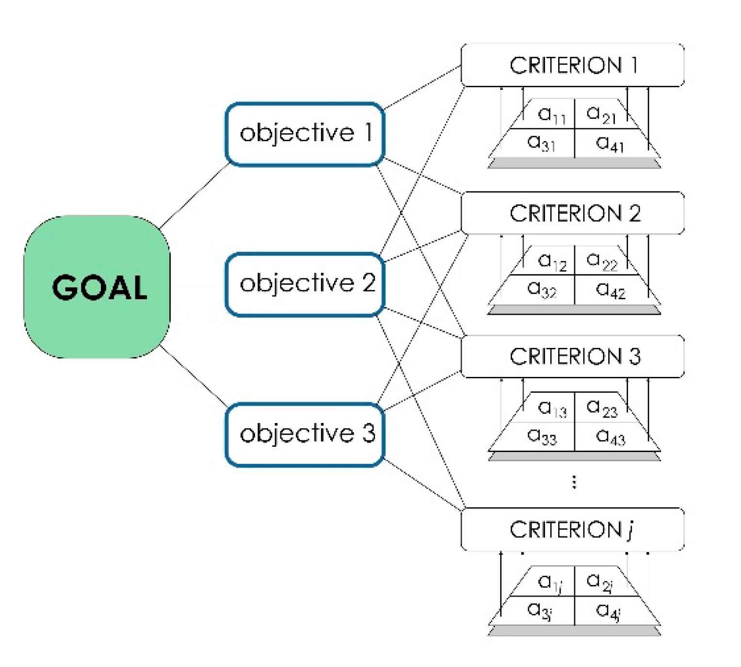
The AHP method determines the objective function V(A_i) using the following rule:

$$V\left(A_i\right)={\displaystyle \sum }_{j=1}^n{w}_k{w}_{j\left(k\right)}v(a_{ij})$$

(8)

where:

• $w_k$—the weight determined by the paired comparison method and related to the k-th objective (k = 1, 2, …, p),
• $w_{j\left(k\right)}$—the weight determined by the paired comparison method and assigned to the j-th criterion related to the k-th objective,
• $v(a_{ij}$)—the value function.

It is assumed that the best alternative is the one having the highest value V(A).

The AHP method, in combination with geographic information systems, is a convenient and useful tool used in the process of making location-related decisions. This includes the analysis conducted for the purposes of the wind farm location [55,56], where the AHP method was used to estimate the weights for the maps of particular criteria values. These maps are combined using the spatial linking rules, e.g., WLC (weighted linear combination) [31,40]. The AHP method was also applied to assess the intensity of the investment potential location based on its planning and infrastructural features and on the features resulting from the current use [53]. Here, the preferences for all the levels of the hierarchical model structure were analysed for the purposes of supporting the decision-making process.

Malczewski and Jaroszewicz [31] distinguish two groups of solutions linking the AHP and GIS:

• group 1—contains GIS-AHP systems that enable the estimation of criteria weights using the principle of comparative assessment but do not allow the two remaining principles to be met, namely the decomposition of the decision-making problem to the hierarchical structure and the calculation of the objective function value. The problem of the integration of GIS and the AHP analysis methods for the purpose of supporting decision-making processes was also addressed by Jankowski [57], Jun [58], and Kobryń [59], as well as Ozturk and Batuk [55].
• group 2—is the GIS-AHP category, i.e., systems based on all the three AHP principlesmentions the following examples here: Common GIS [59], ILWIS-SMCE [60], or the Ecosystem Management Decision Support System (Criterion Decision Plus) [61,62].

3. Materials and Methods

The study, which allowed the set objectives to be met, was conducted throughout the country. The choice of Poland was dictated both by the fact that the climate is characterised by a high variability of weather conditions and by the dynamic changes in terms of the share of renewable energy in the total primary energy generation. In the years 2016–2020, this index increased from 13.76% to 21.59% [63]. Thus, the conducted analysis may contribute to the optimisation of the energy generation from renewable sources, a field in which Poland is still far behind compared to other European countries.

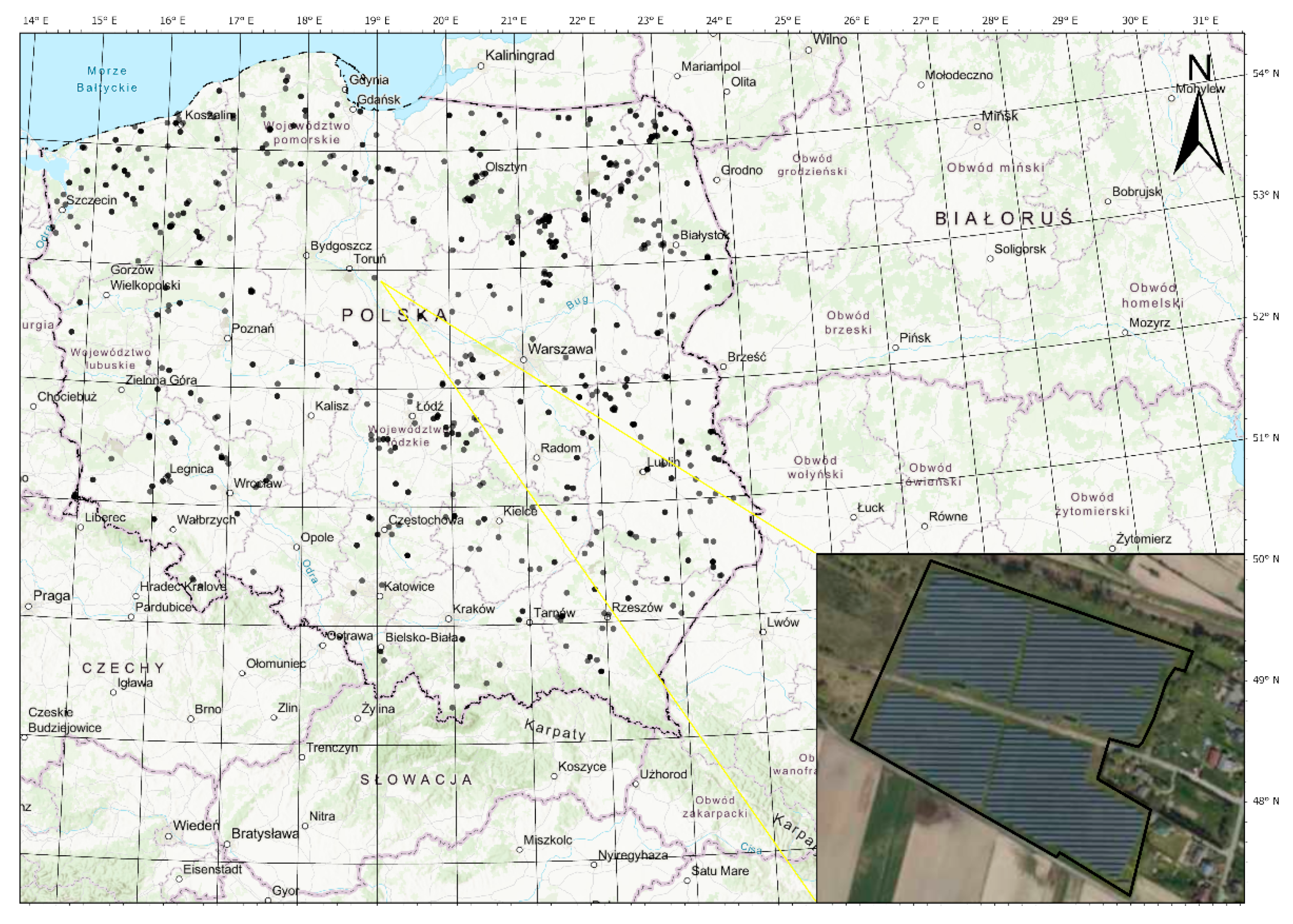
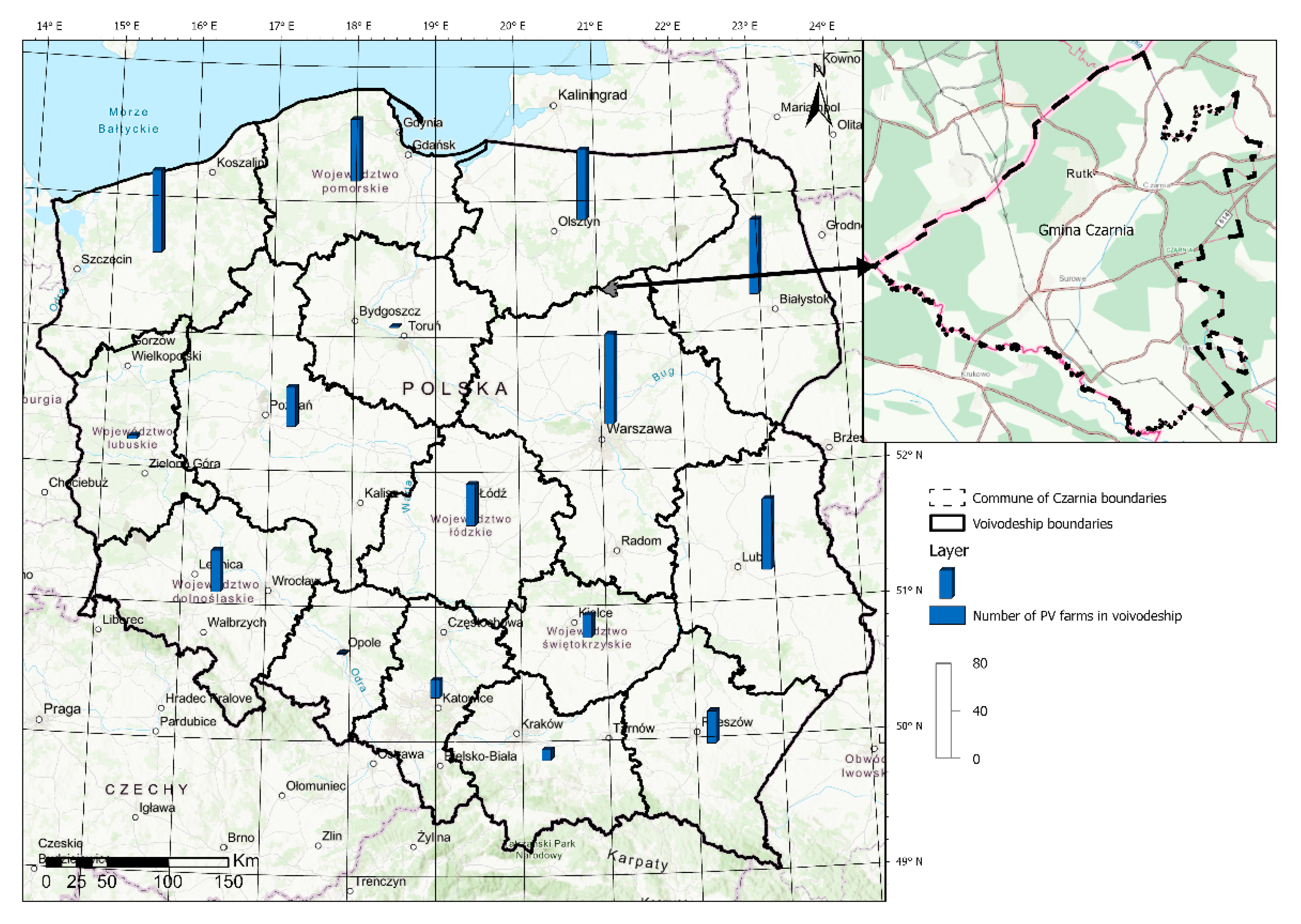
In order to identify photovoltaic farms in Poland, both raster and vector data from the databases of the National Land Surveying and Cartographic Resource were used, supplemented with the OpenStreetMap open data. In the course of the study, it was determined that the presented data did not fully represent the current state, in particular as regards the most recent investment projects of this type. Therefore, the data concerning the photovoltaic farm construction permits issued in the years 2016–2021 were used in order to verify the location of farms that were not included in the existing databases. These locations, i.e., the missing objects, were inserted onto the map (for the vector model) after the visual verification of the available optical imagery (orthophotomap). Finally, a total of 555 photovoltaic farms were localised. The study area and the identified PV farm locations are shown in Figure 4.

Poland (with its diversity of terrain, the degree of investment (industrialisation) and climatic conditions) was selected as a representative study area for Central European countries. The choice of the area under consideration was supported by the availability of spatial data that had been considerably facilitated in recent times, including the use of web services.

3.1. Photovoltaic Farm Location Factors

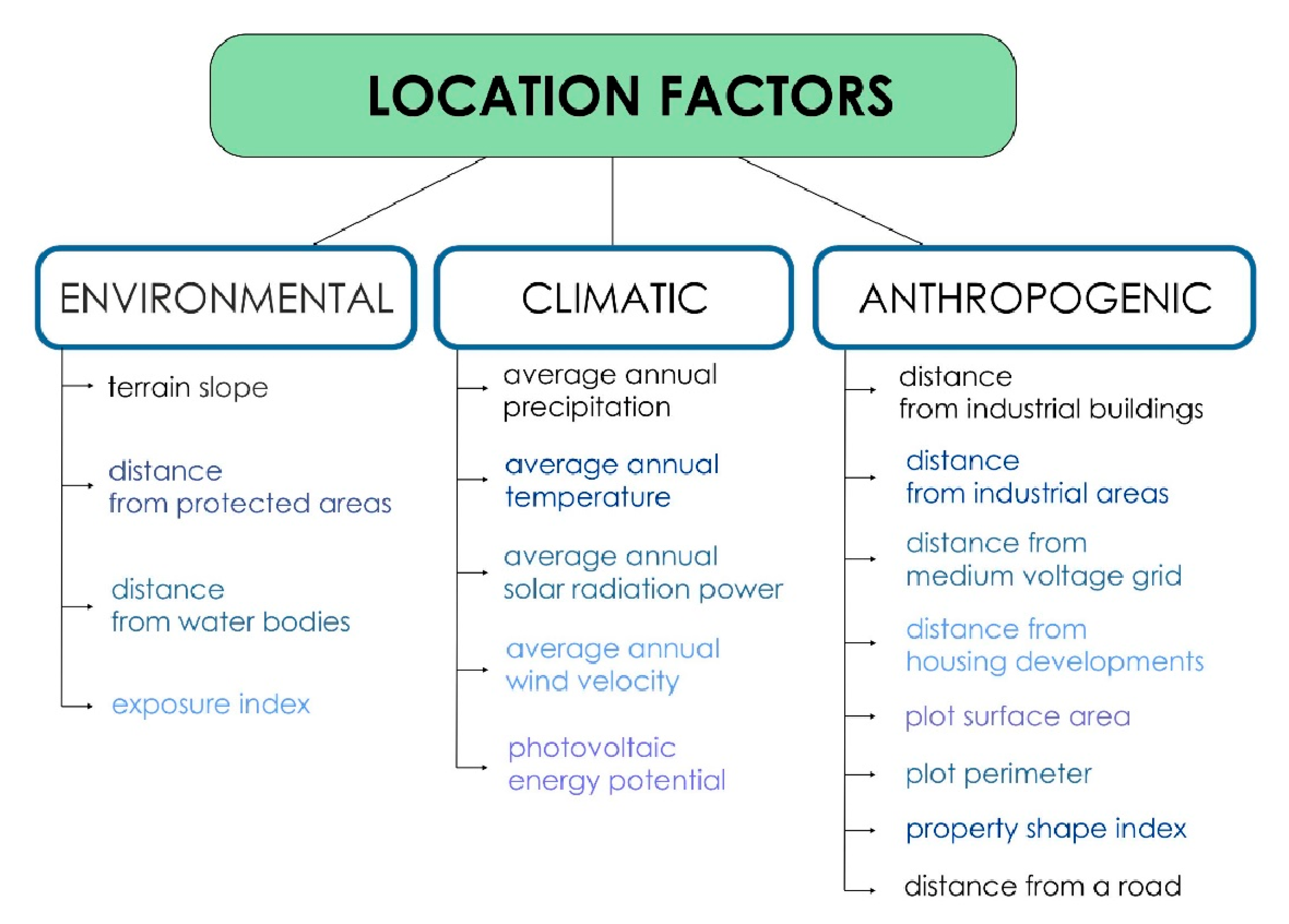
The adopted assumption of the analysis of the location of photovoltaic farms existing throughout the country forced the researchers to thoroughly analyse the actual state of the space. The factors that were identified as crucial in terms of the impact on the location were defined based on the literature review and expert opinions (Section 1). To this end, the authors decided to use datasets, particularly those made available in the vector form, which enables a thorough analysis regardless of the scale and resolution of data. Given that research into the optimisation of the photovoltaic farm location has been often presented in scientific papers, the authors opted for a greater “precision” in terms of the inventory and analysis of significant features. The study selected 17 features that had an impact on the PV farm location, including environmental, anthropogenic, and climatic aspects. The first catalogue of features distinguishes the occurring terrain slope, the distance from protected areas of a high natural value, the distance from water bodies, and the land exposure index. As regards the anthropogenic factors, the authors considered the distance from industrial areas, industrial buildings, medium voltage grids, and residential developments, as well as the surface area, the perimeter, and the index of the shape of the property on which the plant was located. Since the second catalogue of features concerned climatic issues, the following were taken into account: the average annual precipitation, the average annual temperature, the average solar radiation power, and the average annual wind velocity. These factors are provided in the summary in Figure 5. At the same time, it was established that forested, wetland, and underwater areas, due to the ownership structure and form of development, were excluded from the possibility of construction of such investment projects.

As regards the factors under consideration, both the data made available in the National Land Surveying and Cartographic Resource and the publicly available satellite data were used. The data arising from planning documents were not taken into account. After a discussion with experts, it was recognised that it would be very difficult to collect these materials and compile them in a meaningful form for the above research. In addition, this information would be incomplete and subject to constant change.

The aspect of shadows caused by the terrain itself or other artificial infrastructures was not included in the study. Indirectly, in the case of installations in built-up areas, this feature was taken into account in terms of distance from existing buildings.

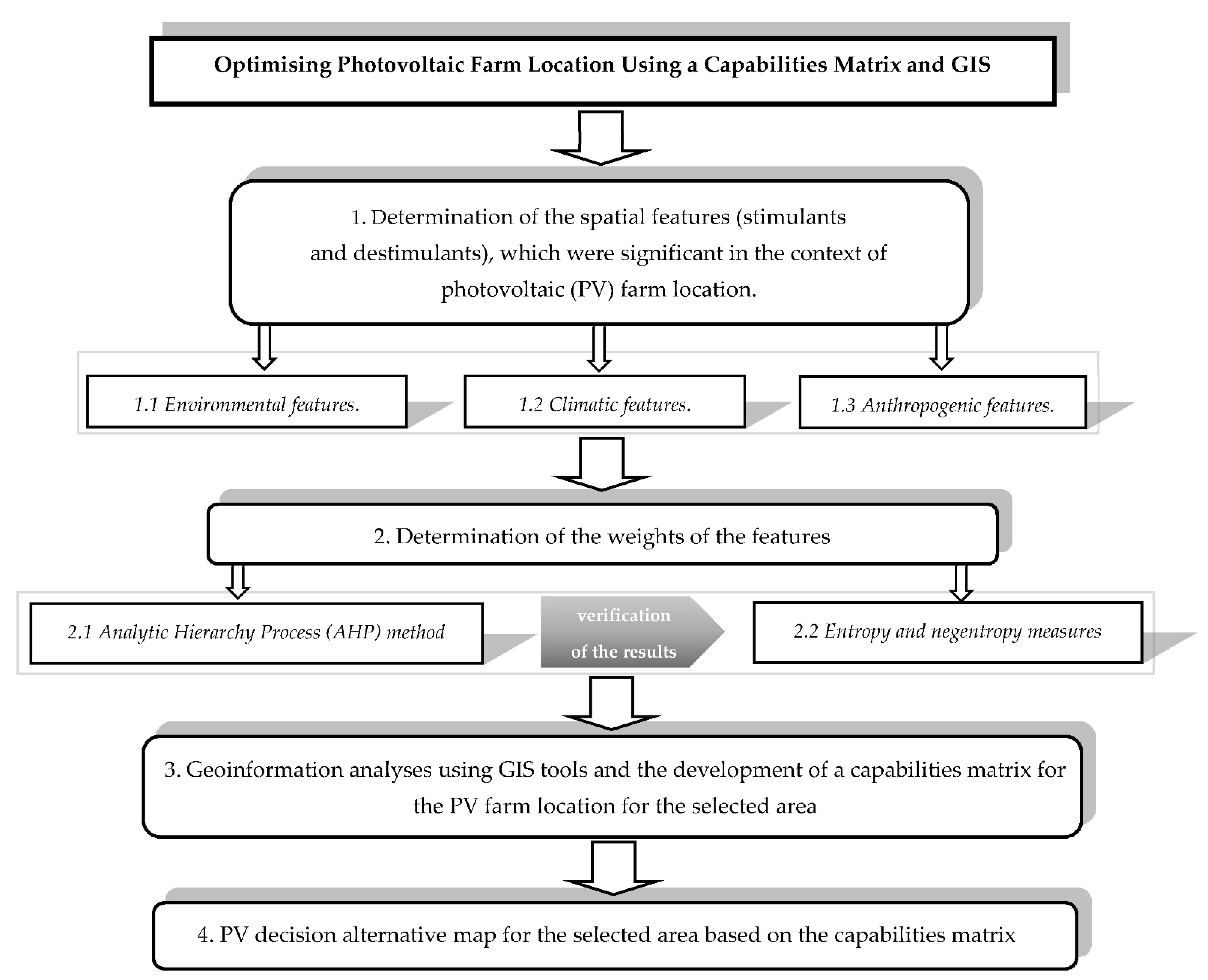
The optimising of photovoltaic farm location using a capabilities matrix and GIS will be conducted according to the procedure presented in Figure 6.

3.1.1. Terrain Slope

The analysis of the inclination of the land for the construction of an investment project, i.e., a photovoltaic farm, is an important element of the investment profitability. On the one hand, overly varied terrain will raise problems in terms of the plant location, while on the other hand, the occurrence of significant differences can be related to costly adaptation earthworks. It should be noted that for the feature under consideration, there are no strict guidelines regarding the land inclination that would be most favourable in terms of the preferred photovoltaic power plant construction site. Therefore, the significance of this feature was verified based on the analysis of 555 farm locations. The topography analysis used data from a numerical terrain model (NTM) obtained from aerial laser scanning (ALS) with a 1 m × 1 m grid (

Table A1. Table with data sources.

Criteria	Source	Reference System	Resolution	Scale	Distribution	Format	URL
Terrain slope	Digital Terrain Model	EPSG:2180	1 m × 1 m	-	Poland	raster	https://mapy.geoportal.gov.pl/wss/service/PZGIK/NMT/GRID1/WCS/DigitalTerrainModel (accessed on 8 September 2022)
Distance from protected areas	Central Register of Nature Conservation Forms	EPSG:2180	-	1:10,000	Poland	vector	https://sdi.gdos.gov.pl/wfs (accessed on 8 September 2022)
Distance from surface water	Database of Topographic Objects	EPSG:2180	-	1:10,000	Poland	vector	https://mapy.geoportal.gov.pl/wss/service/PZGIK/BDOT/WMS/PobieranieBDOT10k (accessed on 8 September 2022)
Exposure index	Digital Terrain Model	EPSG:2180	1 m × 1 m	-	Poland	raster	https://mapy.geoportal.gov.pl/wss/service/PZGIK/NMT/GRID1/WCS/DigitalTerrainModel (accessed on 8 September 2022)
Average annual precipitation	WorldClim v2	EPSG:4326	30 arc-second	-	Global	raster	https://www.worldclim.org/data/worldclim21.html (accessed on 8 September 2022)
Average annual temperature	WorldClim v2	EPSG:4326	30 arc-second	-	Global	raster	https://www.worldclim.org/data/worldclim21.html (accessed on 8 September 2022)
Average annual solar radiation power	WorldClim v2	EPSG:4326	30 arc-second	-	Global	raster	https://www.worldclim.org/data/worldclim21.html (accessed on 8 September 2022)
Average annual wind velocity	WorldClim v2	EPSG:4326	30 arc-second	-	Global	raster	https://www.worldclim.org/data/worldclim21.html (accessed on 8 September 2022)
Photovoltaic energy potential	Solargis	EPSG:4326	30 arc-second	-	60° N–50° S	raster	https://solargis.com/maps-and-gis-data/overview (accessed on 8 September 2022)
Distance from industrial buildings	Database of Topographic Objects	EPSG:2180	-	1:10,000	Poland	vector	https://mapy.geoportal.gov.pl/wss/service/PZGIK/BDOT/WMS/PobieranieBDOT10k (accessed on 8 September 2022)
Distance from industrial areas	Database of Topographic Objects	EPSG:2180	-	1:10,000	Poland	vector	https://mapy.geoportal.gov.pl/wss/service/PZGIK/BDOT/WMS/PobieranieBDOT10k (accessed on 8 September 2022)
Distance from medium voltage grid	Database of Topographic Objects	EPSG:2180	-	1:10,000	Poland	vector	https://mapy.geoportal.gov.pl/wss/service/PZGIK/BDOT/WMS/PobieranieBDOT10k (accessed on 8 September 2022)
Distance from housing developments	Database of Topographic Objects	EPSG:2180	-	1:10,000	Poland	vector	https://mapy.geoportal.gov.pl/wss/service/PZGIK/BDOT/WMS/PobieranieBDOT10k (accessed on 8 September 2022)
Plot surface area	Land and Property Register	EPSG:2180	-	1:5000	Poland	vector	https://integracja.gugik.gov.pl/cgi-bin/KrajowaIntegracjaEwidencjiGruntow (accessed on 8 September 2022)
Plot perimeter	Land and Property Register	EPSG:2180	-	1:5000	Poland	vector	https://integracja.gugik.gov.pl/cgi-bin/KrajowaIntegracjaEwidencjiGruntow (accessed on 8 September 2022)
Property shape index	Land and Property Register	EPSG:2180	-	1:5000	Poland	vector	https://integracja.gugik.gov.pl/cgi-bin/KrajowaIntegracjaEwidencjiGruntow (accessed on 8 September 2022)
Distance from a road	Database of Topographic Objects	EPSG:2180	-	1:10,000	Poland	vector	https://mapy.geoportal.gov.pl/wss/service/PZGIK/BDOT/WMS/PobieranieBDOT10k (accessed on 8 September 2022)

). The terrain slope analysis considered the area representing a buffer zone with a radius of 30 metres from the plant. Adopting a larger area to be analysed enabled the determination of the extent to which the area in question had previously been characterised by favourable topography conditions. As part of the analysis, after calculating the terrain slope using ArcGIS Pro software, the data were converted from the raster format into the vector format. In the next step, the terrain slope obtained was weighted using the surface of the area to which the appropriate land inclination value was assigned. This enabled the calculation of the dominant slope inclination value in relation to individual photovoltaic farms. The average value obtained for the analysed dataset was 1.37°.

3.1.2. Distance from Protected Areas

Consideration of nature conservation forms when locating photovoltaic farms is a particularly important issue. This is due to the fact that environmental legislation excludes the possibility of photovoltaic farm construction in certain areas and makes it much more difficult in other areas due to restrictions being introduced. When analysing the factor concerning the distance from naturally valuable areas, the General Directorate for Environmental Protection data were used (Table A1). The data in the vector format that were made available concerned the following nature conservation forms:

• National Parks
• Landscape parks
• Nature reserves
• Nature parks
• Nature and landscape complexes
• Ecological sites
• Documentation sites
• RAMSAR
• Surface natural monuments
• Ecological corridors

Of all the objects under consideration, 98 farms were located in naturally valuable areas. Therefore, it should be noted that this is not a factor that fully excludes the possibility of location but is both procedurally and socially related to the extended procedure. In view of the above, it was decided to analyse the factors related to naturally valuable areas.

3.1.3. Distance from Surface Water

As regards the analysis of the factor concerning the distance of the plant from surface water, both the possibility of flooding and the increased air humidity were taken into account. The air humidity reduces the output power of photovoltaic panels by reducing the amount of solar radiation received [64]. However, when combined with an appropriate wind velocity, the humidity enables the cooling of panel surfaces, thus increasing their efficiency during warm periods of the year [65]. It should be noted that there is also an element which, as required by environmental legislation, is analysed in the environmental impact report. The analysis concerned used the vector data that make up the Database of Topographic Objects for compilations at a scale of 1:10,000 (BDOT10k) (Table A1). For the purposes of the study, the data concerning surface water were acquired for the entire country by means of integrating databases from individual powiats (counties). The accuracy of the position of objects in the set under analysis is 1 metre. However, the procedure for updating topographic data assumes that this type of work should be performed once every three years.

3.1.4. Exposure Index

Another important factor related to terrain is exposure. In addition to the information on slope inclinations, the exposure of slopes in relation to the sides of the world for any terrain on which a photovoltaic plant is located allows the panels to be installed effectively. The topography analysis used data from a numerical terrain model (NTM) obtained from aerial laser scanning (ALS) with a 1 m × 1 m grid (Table A1). The application of aerial scanning technology allows a high accuracy of the developed elevation data to be obtained. The slope exposure analysis considered the area representing a buffer zone with a radius of 30 metres from the plant. The analysis adopted eight exposure division classes:

• south (S),
• south-east (S-E),
• east (E),
• north-east (N-E),
• north (N),
• north-west (N-W),
• west (W),
• south-west (S-W).

As part of the analysis of the exposure of the objects under consideration using ArcGIS Pro software, the data was converted from the raster format to the vector format, assigning them to the above-mentioned individual classes. In the next step, the polygons obtained were weighted using the surface of the area to which the appropriate land exposure value was assigned. This enabled the determination of dominant values in relation to the total surface area under consideration for particular photovoltaic farms.

3.1.5. Average Annual Precipitation

The first analysed factor that includes climatic data is the quantity comprising the average annual precipitation. Each photovoltaic plant is based on panels which allow energy to be obtained from the Sun’s rays. Thus, it should be an element that, due to its strength, demonstrates its resilience even under extreme weather conditions. When analysing the hazards and benefits arising from the nature of the precipitation, it should be noted that increased precipitation during the winter period may result in a risk of damage or reduced performance of the entire plant. On the other hand, in spring and summer, significant amounts of airborne pollutants in the form of dust and pollen, which deposit on the panels and thus reduce their performance, can be removed spontaneously by rain. The data in the raster form used in the analysis were acquired from the WorldClim dataset [66]. Of all the materials made available, the study also used sets with a spatial resolution of 30 s (~1 km²) (Table A1). The data presents summaries for average annual measurements compiled for the period from 1970 to 2000. The average values expressed in mm for 555 locations of photovoltaic farms were obtained by means of raster sampling.

3.1.6. Average Annual Temperature

The variability rate for the weather conditions under which the temperature values are also analysed affects the efficiency of photovoltaic systems [64]. It should be noted that a change in the temperature affects the light absorption efficiency and, consequently, the volume of energy generated. In order to determine the average annual temperature expressed in °C for the photovoltaic farms under consideration, the raster data available in the WorldClim dataset were used [66]. The resolution of the spatial dataset was 30 s (~1 km²) (Table A1). The data for the analysed photovoltaic plants were acquired by sampling the raster data.

3.1.7. Average Annual Solar Radiation Power

The data on solar radiation in particular regions of the country in which the photovoltaic farms under consideration are located were derived in the raster form from the WorldClim dataset [66]. The data acquired in kJ m⁻² day⁻¹ for spatial resolution of 30 s (~1 km²) enabled the identification of areas with high values of this index (Table A1). Optimisation in terms of the photovoltaic farm location for this factor will obviously be related to the selection of areas with higher values. The analysis of the existing photovoltaic farms yielded values for each location by means of raster sampling.

3.1.8. Average Annual Wind Velocity

An important factor in analysing the location of photovoltaic plants is the wind velocity values found in a particular area. By cooling the panels, the factor concerned allows higher panel efficiency values to be obtained by reducing the resistance [67]. On the other hand, gusts of wind can carry significant amounts of dirt, i.e., dust or sand, onto the panels. It should also be noted that strong gusts of wind can damage photovoltaic panels when installed incorrectly. The data in the raster form, showing the wind velocity in ms⁻¹, were derived from the WorldClim dataset [66] (Table A1). The spatial data resolution was 30 s (~1 km²) and, through the raster sampling, enabled the determination of an average value for individual photovoltaic plants.

3.1.9. Photovoltaic Energy Potential

A factor that was also taken into account is the potential of the average annual electricity production from photovoltaics, developed based on the global solar model Solargis. This index enables the evaluation of the energy production potential for a free-standing photovoltaic power plant at any location in the world. This is the index that should be analysed in the first place, as building photovoltaic plants on low-potential land conflicts with future plant performance. In the model under consideration, the data expressed in kWh/kWp include archive data from the years 1994–2018. The data were acquired in the raster form from the Global Solar Atlas application [68] (Table A1). The value for each of the analysed locations was determined based on the raster sampling.

3.1.10. Distance from Industrial Buildings

In terms of the photovoltaic farm location, the nature of the development found in the vicinity is an important consideration due to possible spatial conflicts as regards the location of the plant close to residential buildings. Therefore, the authors decided to analyse the effect of the distance from industrial buildings, which can, in principle, generate lesser problems as regards the location in the vicinity of photovoltaic plants. Another argument in favour of locating such facilities in the vicinity of industrial buildings is the possibility of diversifying energy sources. For the purposes of developing the index in question, the vector data that make up the Database of Topographic Objects for compilations at a scale of 1:10,000 (BDOT10k) were used (Table A1). This database is a uniform compilation for the entire country, which, with regard to updating the location of buildings and their attributes, is primarily based on the Land and Property Register records. As for the non-inventoried objects, both these and their attributes are entered from field surveys as part of the update, which should be performed at least every three years.

3.1.11. Distance from Industrial Areas

The authors considered the aspect of reusing industrial areas for the construction of photovoltaic plants. Areas previously seen as unusable can provide ideal locations for photovoltaic plants [69]. The use of areas such as industrial brownfield sites or abandoned mining land for the purpose concerned is easier due to their large surface area and industrial nature, allowing social conflicts to be minimised. In addition, arguments for the use of industrial brownfield sites include the absence of the need to dismantle and remove the site’s extensive underground infrastructure, the lack of vegetation, and the possibility of using land degraded by industrial activities. Industrial areas for the entire country were derived from the vector data making up the Database of Topographic Objects for compilations at a scale of 1:10,000 (BDOT10k) (Table A1).

3.1.12. Distance from Medium Voltage Grid

The distance of a photovoltaic plant from a medium voltage power line is of importance in terms of the distribution of the electricity generated. The relationship occurring in this case indicates that the greater the distance from substations and transmission lines, the higher the investment project cost is. Taking into account the distance from the lines will help avoid considerable initial costs, and for the already determined location, it will allow the entire investment project to be calculated correctly. The data used to determine the index in question for the entire country were derived from the Database of Topographic Objects for compilations at a scale of 1:10,000 (BDOT10k) (Table A1). One of the elements in the database in question is the presence of utility networks, including power lines, which are updated at the level of each powiat (county) in the country using local Geodetic Utility Networks (GESUT). The data acquired in the vector format enable the presentation of the current state of the network route.

3.1.13. Distance from Housing Developments

The distance from housing developments is of importance in both the social and spatial aspects. On the one hand, a photovoltaic plant located too closely may lead to public protests. On the other hand, it can contribute to the diversification of the sources of energy that can be used by the housing development residents. The construction of a photovoltaic power plant in close proximity to a housing development in the future may represent a major constraint on the development of residential areas due to the blocking up of the site. The data for the purposes of this study were derived in the vector form from the Database of Topographic Objects (Table A1), which, as in the case of industrial buildings, were based on the Land and Property Register records and field surveys.

3.1.14. Plot Surface Area

The legal status of the inventoried objects was analysed, taking into account the course of the boundaries of the property on which they were located. The authors decided to analyse the size of the plots using the Land and Property Register data made available for the entire country in the vector format (Table A1). It should be noted that the actual surface area of a photovoltaic farm often did not correspond to the cadastral surface area of the property. The authors decided to analyse this aspect as, at the time of investment project implementation, it is the surface area of the plot that determines the possibilities for the location of a particular object.

3.1.15. Plot Perimeter

As in the case of the plot area, this feature related to the location of a photovoltaic plant was determined based on the uniform and consistent Land and Property Register that covers the scope of the entire country. To acquire the data, the authors decided to use the vector data made available as part of the WFS (Web Feature Service) online download service. The data are transmitted in the GML (Geography Markup Language) format (Table A1), which can be exported into any vector format using GIS software. For the purposes of the study, the authors assumed that the perimeter allows the plot shape to be described as a significant feature when selecting properties for the construction of photovoltaic plants.

3.1.16. Property Shape Index

Another variable analysed in the context of inventoried photovoltaic farms is the property shape. For the purposes of this study, the determination of property shape based on the relationship between its surface area and the perimeter was adopted (Table A1). To this end, the formula [70] used was:

$$W_k=40\ast \pi \ast \frac{P}{O^2}$$

(9)

where:

• W_k—shape index,
• P—property surface area,
• O—property perimeter.

The index described by Formula (9) is standardised in the interval of (0; 10>. The value of 10 will be obtained for the figure of a circle, while 0 for an infinitely elongated figure. As regards the objects under analysis, a figure that is optimal in terms of developability is a square for which the value of the calculated index amounts to 7.85. Therefore, the lower the value, the more irregular and elongated the shape of the property is, and thus the greater problems emerge in terms of the optimal use of the entire area for the construction of a photovoltaic plant.

3.1.17. Distance from a Road

The authors decided, as in the case of any technical infrastructure investment project, to analyse the accessibility of public roads. In this regard, the analysis covered both the stage of the photovoltaic farm construction and the subsequent stage of its operation. The close proximity to roads enables both an easy delivery of materials at the construction stage and easy access for those involved in plant maintenance and servicing. In order to correctly verify the particular feature, the authors used the data for the entire country, derived from the Database of Topographic Objects for compilations at a scale of 1:10,000 (BDOT10k) (Table A1). One of the elements in the database in question is the transport network updated at the level of each powiat (county) in the country, using databases of public administration bodies in charge of roads at the national, voivodeship, county, and commune levels. Road registers and records, including the correct routes and descriptions of particular roads, enable the accurate and up-to-date reconstruction of the existing state of the transport network throughout the country. In addition to the indicated data, the obtained data in the vector format also contain information on the management category, thus indicating which of them belong to public roads.

3.2. Determination of the Criterion Weights (PCM and AHP)

The diversity of the analysed 555 cases of photovoltaic plants in terms of the seventeen features under consideration enabled the conclusion that their interrelationships and the hierarchical layout require an appropriate method for determining the significance of particular features in the procedure of selecting the optimum photovoltaic farm location. To this end, the authors decided to employ the AHP (Analytic Hierarchy Process) method, which allows multiple criteria, presented in both the quantitative and qualitative form, to be juxtaposed as part of a single decision-making process. The use of this method, by the juxtaposition of paired comparisons of different features, allows the process of creating the final assessment to be automated. Ultimately, when assessing the features, scholars’ and experts’ opinions contained in the above-cited publications were used, as well as the data on the space collected for the existing photovoltaic plants. The collected criteria were grouped into semantic categories while taking into account their nature and interrelationships. The alignment involved the assignment of natural (environmental), climatic, and anthropogenic location factors to the group. It should be noted that the publications mentioned at the literature analysis stage did not refer to such a large number of variables, in particular in relation to an area characterised by high variability of weather conditions throughout the year.

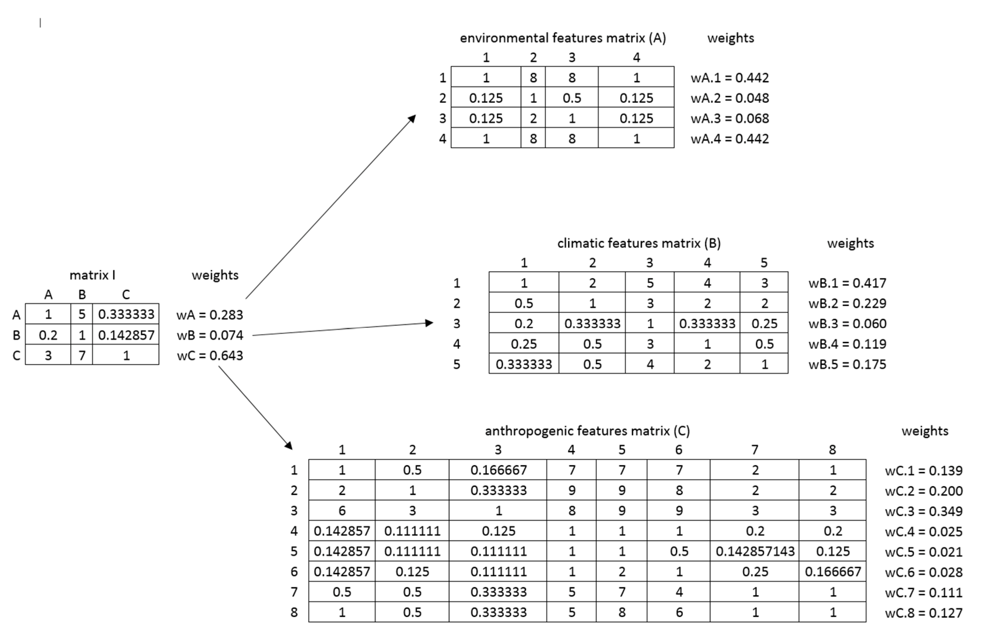
In the adopted methodology, a hierarchical tree comprising two feature detail levels was developed. The most extended sub-group of features was related to the elements of the space associated with anthropogenic activities. Based on the hierarchical grouping of the features, a hierarchical system of matrices was established, in which, according to the AHP principles, the analysed features were subjected to paired comparison. The calculated matrices in the form of a hierarchical tree, along with the calculated values of weights, are provided in the figure (Figure 7).

Then, in order to verify the correctness of the weight calculation, Consistency Indices (CI) and Consistency Ratios (CR) were determined. A summary of CI and CR indices that were calculated for all matrices is provided in the table (

Table 3. A summary of CI and CR indices for the paired comparison matrix.

Hierarchy Level		CI	CR
I	II
Matrix I		0.05	0.09
	Environmental features matrix (A)	0.03	0.04
	Climatic features matrix (B)	0.05	0.04
	Anthropogenic features matrix (C)	0.09	0.06

).

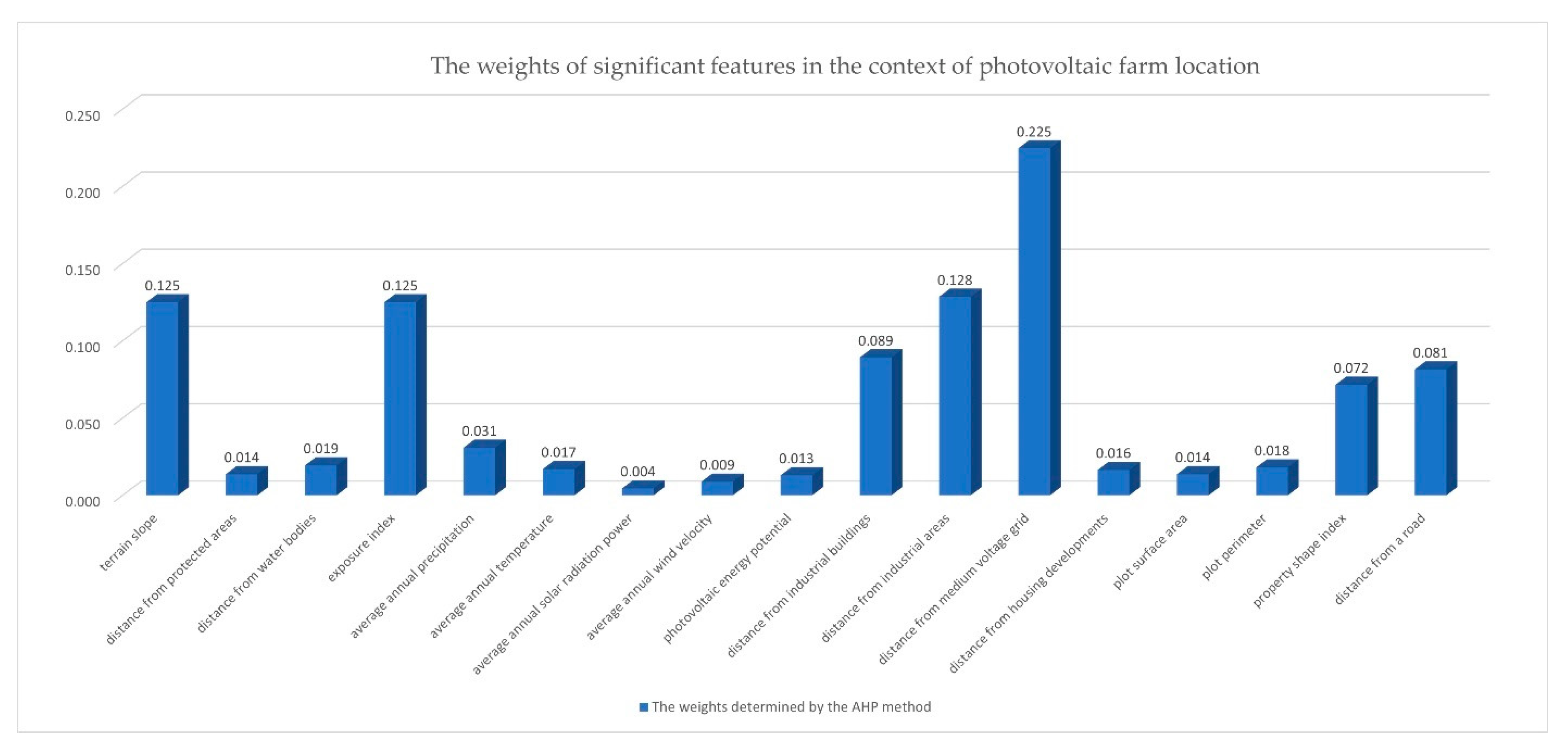
Based on the results obtained, it was concluded that the CR index for all matrices satisfied the condition of <0.1. This led to the next stage of the final determination of the weight values by multiplying them in a hierarchical system. The results are provided in the diagram below (Figure 8).

3.3. Determination of Criteria Weights by the Entropy Method

In order to verify the weight significance, the authors decided to use the measure of the state of disorder, i.e., entropy, to determine the variability of the criteria under analysis. To assess the significance of individual criteria, it was decided to analyse the information carrying capacity within the framework of 555 existing photovoltaic farms under consideration. In order to determine the values for individual features, the data were transformed towards a uniform impact on the PV farm location and then standardised to an interval of values of <0; 1>. Of the various manners of normalisation, the authors chose the one being most congruent to the features due to the value span and the purpose of normalisation. Equations (10) and (11) were used for this purpose:

the stimulants:

$$z{n}_{rj}=\frac{c_{rj}-\min c_j}{\max c_j-\min c_j}$$

(10)

the destimulants:

$$z{n}_{rj}=\frac{\max c_j-c_{rj}}{\max c_j-\min c_j}$$

(11)

where:

• c_rj—values of j-th criterion for r-th field (r = 1, 2, …, m, j = 1, 2, …, n)
• zn_rj—normalised value of j-th feature for r-th field. The normalised values of the features fall within the numerical range of (0, 1).

In the next step, the authors calculated the entropy of each E_j criterion using the formula below (12):

$$E_j=-K{\displaystyle \sum }_{i=1}^m{p}_{ij}\ln p_{ij}$$

(12)

where:

• E_j—entropy of the j-th criterion
• K—the constant calculated from the formula K = 1/lnm
• m—number of objects under analysis (m = 555)
• p_ij—the value of the j-th criterion for the i-th case

In the next step, the weights of individual criteria were calculated using the Equation (13) below:

$$w_j=\frac{d_j}{{{\displaystyle \sum }}_{j=1}^n{d}_j}$$

(13)

where:

• w_j—the weight of the j-th criterion
• d_j—the degree of intrinsic divergence of assessments in relation to successive criteria.

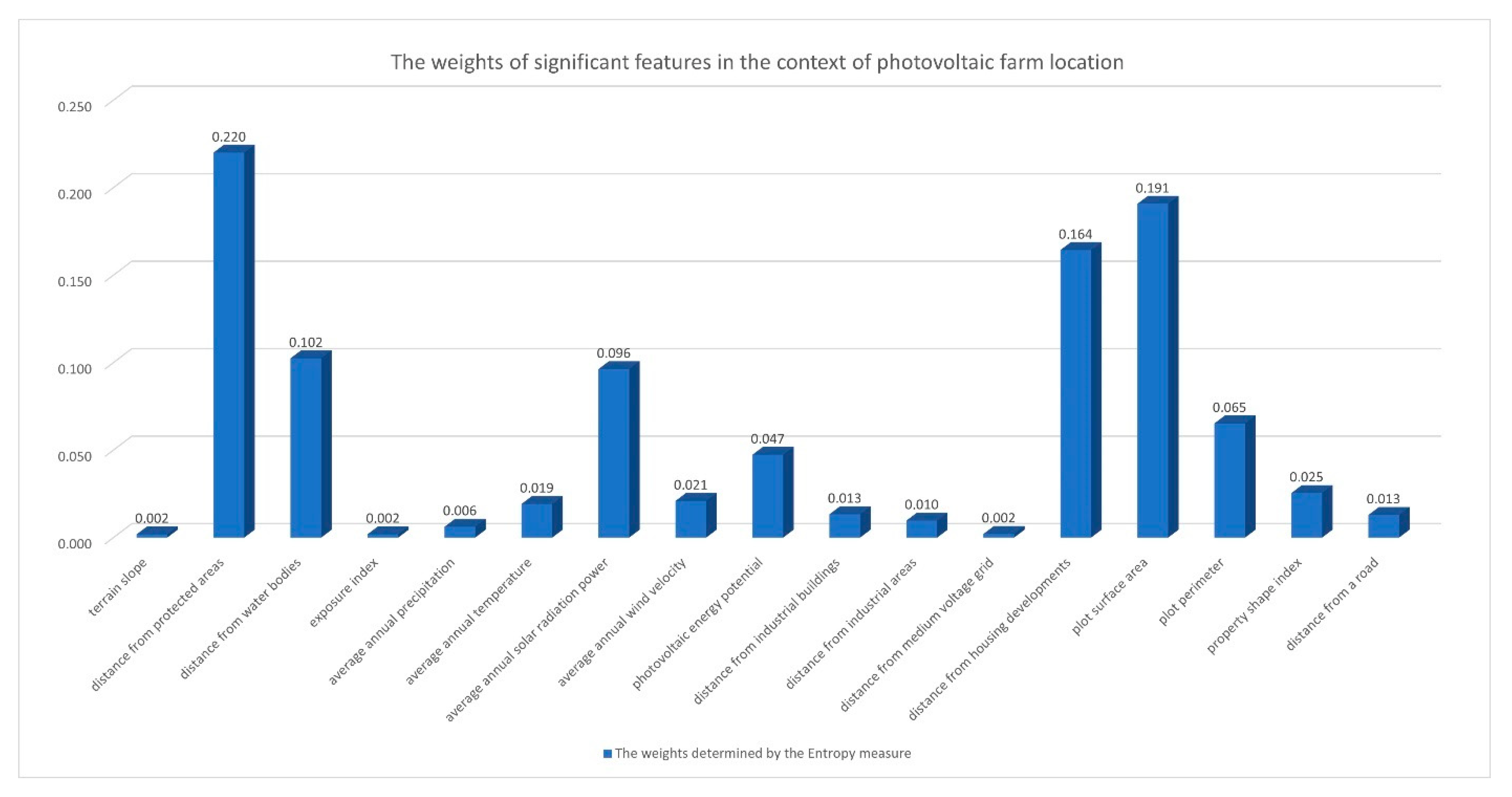
The calculations resulted in the determination of weight values for the criteria under consideration. According to the assumptions, the more diverse information is provided by the j-th criterion, the lower the entropy value is, and thus the greater weight it obtains (Figure 9). Therefore, the more information is provided by the j-th criterion, the more important it is in the assessment.

An important element of the criteria significance assessment using entropy is to be based on the actual data describing the existing photovoltaic farms. By juxtaposing this with a precise representation of the space, which is guaranteed by the National Land Surveying and Cartographic Resource’s data used in the study, the actual determination of the information carrying capacity for particular criteria could be obtained.

4. Results

In order to verify the adopted method, the authors decided to analyse the photovoltaic farm location capabilities in a selected area of the country. To this end, a quantitative analysis of the existing locations of photovoltaic plants was conducted in relation to voivodeships and individual communes. It was found that the highest proportion of photovoltaic plants were present in Mazowieckie Voivodeship, where 76 objects of this type are located (Figure 10).

In view of the above, the authors decided to conduct an analysis on a commune situated in Mazowieckie Voivodeship, which has no such facility (Figure 10). An additional analysis conducted for communes indicated that a total of 23 photovoltaic farms were situated in the communes of Myszyniec and Kadzidło. Based on this fact, the choice fell on the commune of Czarnia, situated in the immediate vicinity of the above-mentioned communes.

The commune under consideration is situated in the northeastern part of Mazowieckie Voivodeship. There are forested areas and surface water in the commune, and the total area of the commune is 93.85 km².

4.1. Capabilities Matrix for the Optimum Photovoltaic Farm Location

The adopted procedure methodology using the AHP method resulted in the plot surface area being regarded as the decision alternative. Due to the spatial determinants, forested areas and land covered with surface water were excluded from the analysis at the first stage. The elimination of certain objects from the analysis in question yielded a set of 6991 properties in the selected commune, for which data for the 17 analysed criteria were later acquired. This resulted in the development of the capabilities matrix (

Table 4. A fragment of the capabilities matrix developed for the selected area (Czernia Commune). In total, this capabilities matrix contains 6990 objects of analysis.

Cadastral Parcels	Terrain Slope	Distance from Protected Areas	Distance from Water Bodies	Exposure Index	Average Annual Precipitation	Average Annual Temperature	Average Annual Solar Radiation Power	Average Annual Wind Velocity	Photovoltaic Energy Potential	Distance from Industrial Buildings	Distance from Industrial Areas	Distance from Medium Voltage Grid	Distance from Housing Developments	Plot Surface Area	Plot Perimeter	Property Shape Index	Distance from a Road	PV farm Location Index
141502_2.0001.1	1	0	0	0.5251	0.8293	0.8333	0.6458	0.4913	0.9527	0.6435	0.6137	0.6023	0.3194	0.0236	0.0441	0.6226	0.7658	0.6345
141502_2.0001.10	1	0	0	0.5182	0.8598	0.8333	0.6731	0.5361	0.9510	0.6485	0.6481	0.6112	0.2550	0.0098	0.0374	0.3559	0.7751	0.6222
141502_2.0001.100	0.9739	0	0.2227	0.4912	0.8993	0.6667	0.6747	0.6608	0.9349	0.5679	0.6549	0.6454	0.3065	0.0049	0.0528	0.0873	0.8183	0.6059
141502_2.0001.101	0.9921	0	0.2203	0.5066	0.9012	0.6667	0.6747	0.6608	0.9318	0.5686	0.6539	0.6440	0.3005	0.0057	0.0552	0.0929	0.8096	0.6093
141502_2.0001.102	0.9923	0	0.2199	0.5342	0.8885	0.6667	0.6767	0.6608	0.9440	0.5686	0.6527	0.5760	0.2887	0.0069	0.0368	0.2584	0.7976	0.6075
141502_2.0001.119/178	0.9646	0.0209	0.2446	0.4262	0.8819	0.6667	0.5916	0.7539	0.8976	0.5275	0.7583	0.6675	0.2094	0.0014	0.0225	0.1352	0.8314	0.6137
141502_2.0001.119/183	0.9976	0.0768	0.2743	0.5041	0.8886	0.6667	0.5972	0.7526	0.8901	0.5136	0.7502	0.7033	0.2029	0.0014	0.0226	0.1342	0.7989	0.6320
141502_2.0001.119/184	0.9596	0.1330	0.3015	0.4308	0.9136	0.6667	0.6237	0.7471	0.8680	0.4996	0.7407	0.7265	0.2047	0.0012	0.0191	0.1547	0.7474	0.6199
141502_2.0001.119/188	1	0.1876	0.3326	0.4161	0.9310	0.6667	0.6472	0.7438	0.8524	0.4860	0.7293	0.7312	0.2324	0.0002	0.0047	0.4945	0.6772	0.6420
141502_2.0001.119/189	0.9649	0.1964	0.3389	0.3828	0.9369	0.6667	0.6562	0.7432	0.8465	0.4839	0.7269	0.7365	0.2389	0.0011	0.0180	0.1650	0.7651	0.6185
141502_2.0001.108	0.9972	0	0.2271	0.5106	0.8844	0.6667	0.6777	0.6608	0.9396	0.5660	0.6413	0.6233	0.2331	0.0088	0.0525	0.1609	0.6778	0.5967
141502_2.0001.109	0.9951	0	0.2440	0.5030	0.8743	0.6667	0.6798	0.6608	0.9501	0.5603	0.6391	0.6192	0.2257	0.0080	0.0436	0.2128	0.6991	0.5991
141502_2.0001.11	1	0	0.0269	0.5423	0.8489	0.8176	0.6645	0.5208	0.9506	0.6341	0.6258	0.5529	0.3511	0.0072	0.0271	0.4943	0.6945	0.6124
141502_2.0001.110	0.9932	0	0.2638	0.4699	0.8881	0.6667	0.6775	0.6608	0.9326	0.5536	0.6366	0.6141	0.2252	0.0058	0.0328	0.2749	0.7036	0.5978
141502_2.0001.111	0.9894	0	0.2899	0.5118	0.8870	0.6667	0.6778	0.6608	0.9317	0.5449	0.6343	0.6095	0.2223	0.0039	0.0202	0.4807	0.7023	0.6153
141502_2.0001.112	0.9849	0	0.2970	0.5089	0.8771	0.6667	0.6788	0.6608	0.9390	0.5425	0.6310	0.6023	0.2114	0.0031	0.0167	0.5545	0.7227	0.6187
141502_2.0001.113	0.9814	0	0.2995	0.4944	0.8809	0.6667	0.6785	0.6608	0.9342	0.5416	0.6282	0.5959	0.2039	0.0021	0.0149	0.4668	0.7349	0.6092
141502_2.0001.114	0.9783	0	0.3023	0.4803	0.8746	0.6667	0.6792	0.6608	0.9384	0.5407	0.6264	0.5917	0.1997	0.0015	0.0133	0.4125	0.7400	0.6022
141502_2.0001.115	0.9799	0	0.3050	0.4417	0.8795	0.6667	0.6787	0.6608	0.9332	0.5398	0.6248	0.5879	0.1975	0.0011	0.0118	0.3992	0.7404	0.5956
141502_2.0001.116	0.9613	0	0.3087	0.4483	0.8771	0.6667	0.6789	0.6608	0.9348	0.5386	0.6236	0.5850	0.1958	0.0022	0.0123	0.6947	0.7391	0.6142

), which the authors used to calculate the optimum PV farm location index value.

As part of determining the value of the optimum PV farm location index for particular cadastral parcels representing decision alternatives, the individual feature values were recalculated using the weights determined by the AHP method.

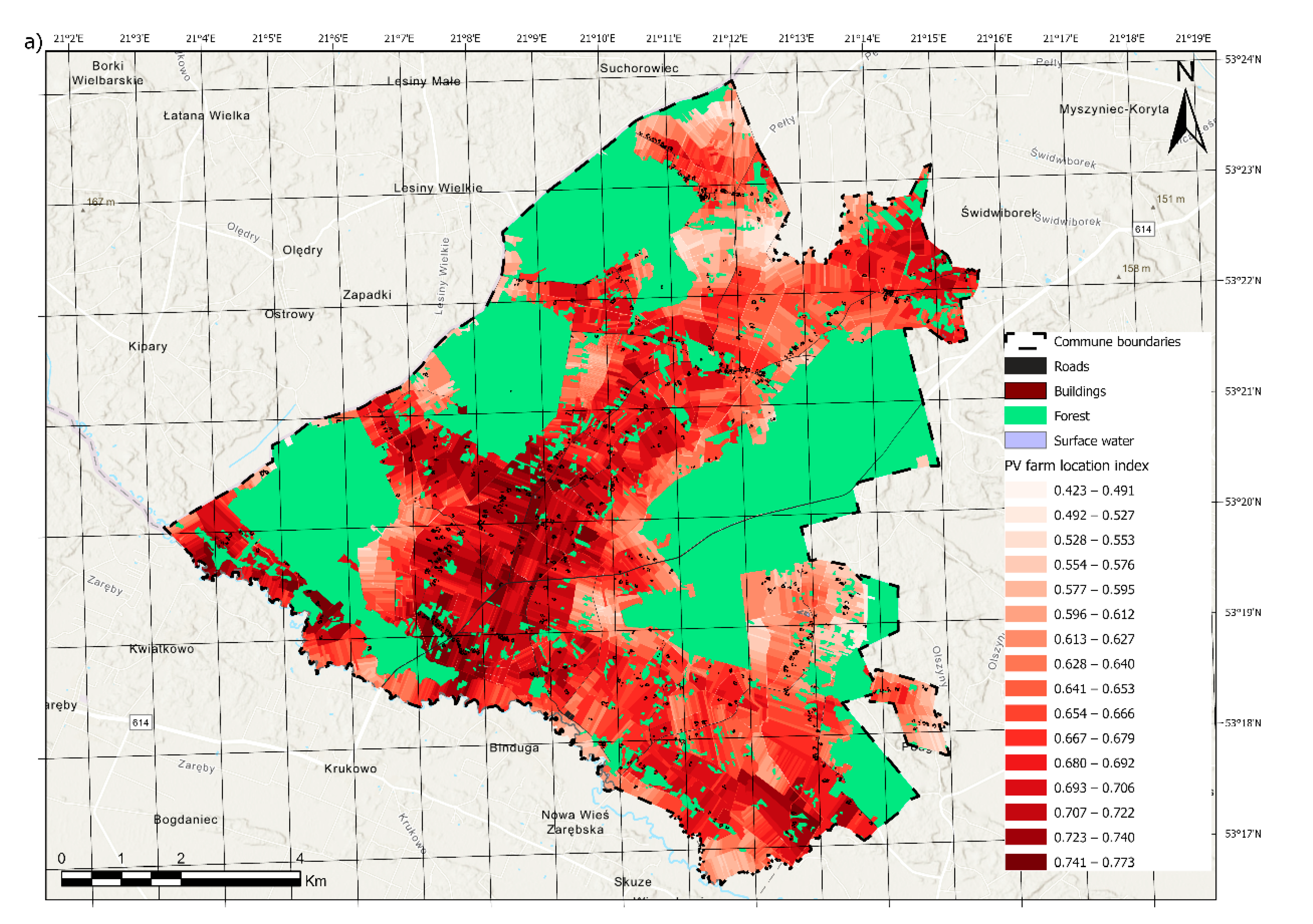
4.2. Map of Decision Alternatives for the Location of PV Farms

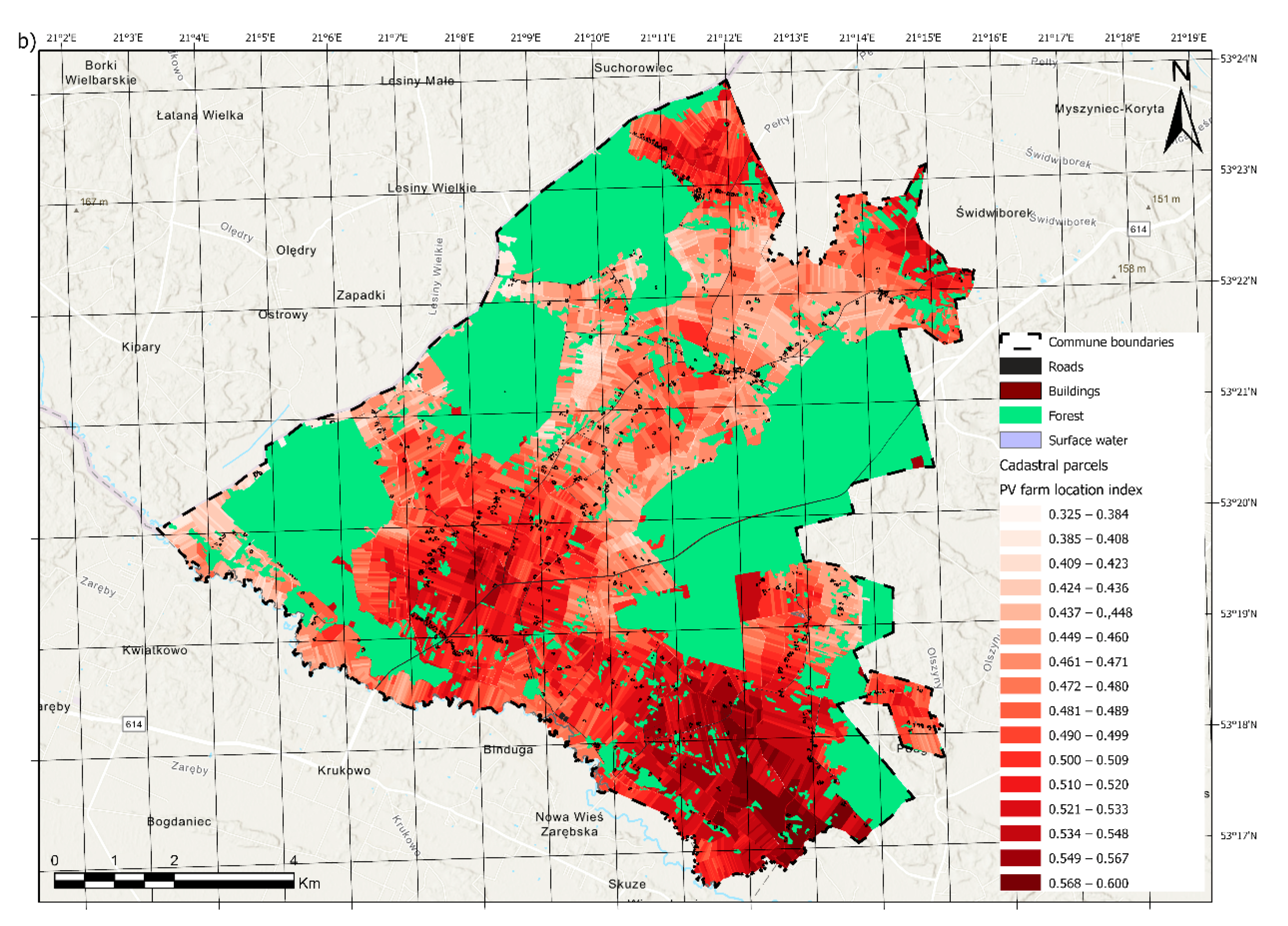
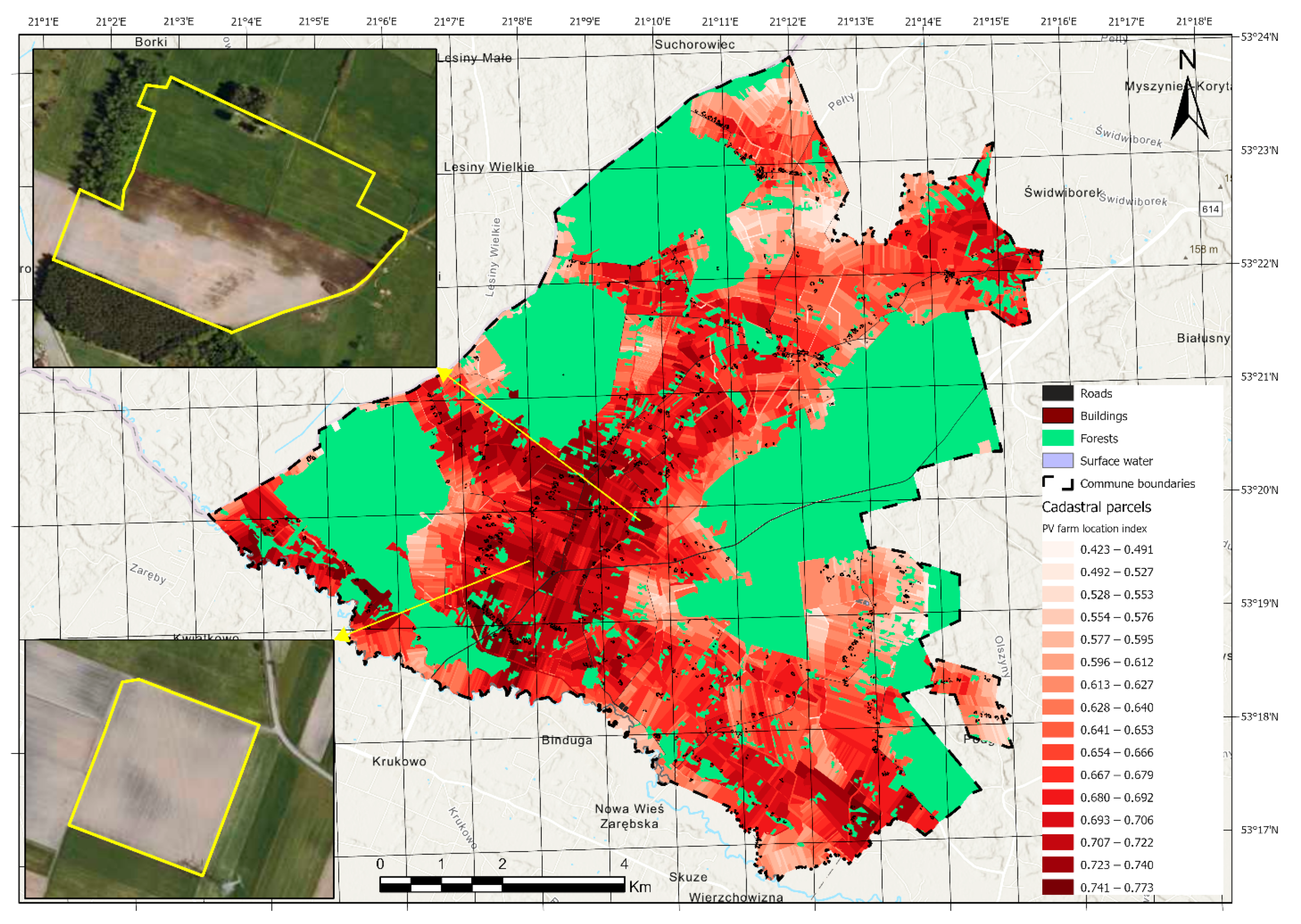
The analysis resulted in the selection of 176 cadastral plots for which the PV farm location potential index was the highest (Figure 11). The objects, based on the analysed set of features after recalculating them by the weights determined by the AHP method, obtained values from the interval (0.741; 0.773). According to the results obtained, it can be concluded that cadastral plots with optimal features for the construction of a photovoltaic farm account for approx. 3% of all objects with a total area of approx. 158 ha in the commune under consideration. Having analysed this in relation to the average surface area of a photovoltaic plant, calculated based on the 555 existing objects, which amounts to approx. 2 ha, one can indicate, in the area under analysis, 18 cadastral plots with an area larger than 2 ha, for which the PV farm location index takes on the highest values.

5. Discussion

Geospatial data are a significant source of information with regard to spatial analyses of the optimum use of renewable energy sources. Nowadays, with unlimited access to newly established and updated spatial data sets combined with modern GIS software, we have the capacity to conduct complex analyses regarding the optimal location of investment projects in the field of technical infrastructure. Certainly, data redundancy generates problems, mainly in terms of selecting an appropriate set and range of data to analyse the selected phenomenon or process. Variation in terms of accuracy, data timeliness, and spatial resolution is an important element that is subject to verification at the initial stage of any spatial inventory analysis. Another element that needs to be determined at the initial stage of work is the choice of interpretation pattern for selected datasets. On the one hand, analysing datasets containing a significant volume of information, such as satellite images, is time consuming and requires a team of specialists. On the other hand, automatic classification frequently using elements of artificial intelligence is not resistant to errors arising from the spatial diversity and the spatial “context” of the neighbourhood. When analysing the capabilities and limitations of these two methods, the authors decided to combine the capabilities of the two above-mentioned algorithms of proceedings in their analyses. Through an analysis of the existing photovoltaic plants, they identified a set of features that need to be taken into account as regards the location of the investment project in question. They then automatically generated sets of data that could be used at the stage of calculating the optimum PV farm location index. Taking the considerations a step further, it should be noted that the tested method can be further automated in a situation in which the weights of individual features of the optimum location are known. In the long term, this will reduce the time it takes to find an optimum location and provides an opportunity to monitor the space in terms of the accessibility of a particular site for the potential investment project on a particular day.

The study demonstrated the validity of applying the AHP method in which the optimum location selection parameters were developed based on the 555 existing photovoltaic plants throughout the country. Based on the existing publications, experts’ opinions, and usable geospatial datasets, a catalogue was compiled of 17 features determining the indication of an optimum cadastral plot for the construction of a photovoltaic farm.

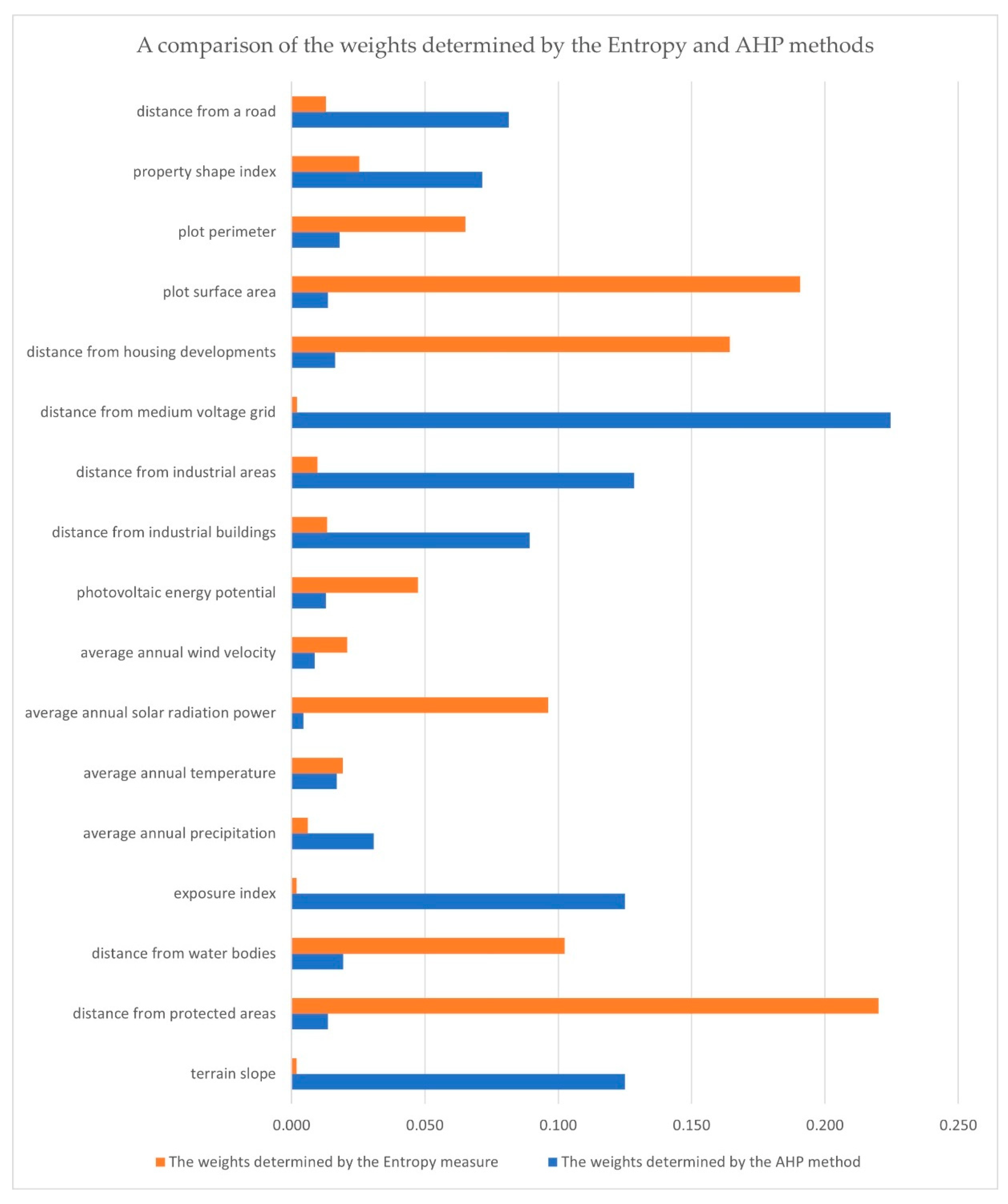
In order to correct the weights determined in the scope of the AHP method, the authors decided to examine the information carrying capacity for individual criteria. To this end, the entropy measure was used, which enabled the determination of variability of the individual criterion values. On this basis, their weights were determined. The weight values were calculated based on the inventoried values of individual features of the 555 photovoltaic plants existing across the country. The quantities determined were intended to be used to correct the weights determined when using the AHP method. Having compared the determined weight according to the two methods, a regularity was established, which is provided in the diagram below (Figure 12).

In analysing the summary of weights, one may note an inverse correlation, according to which the features characterised by high weight values under the AHP method exhibit a low entropy value. It can be concluded that the criteria which are significant from the AHP method perspective show a low variation of information and thus obtain a lower entropy value. When comparing the maps of decision alternatives determined according to the weights identified by the AHP and entropy methods, it is noticeable that the trends in selecting optimum locations for PV farms are, to a certain extent, convergent. As regards the analysis concerning the inclusion of the weights determined based on the entropy values in the model (Figure 13b), 128 cadastral plots with the highest assigned values of the PV farm optimum location index, from the interval of (0.369; 0.438>, were indicated. The smaller number of plots selected by the entropy-based method also translates into a smaller surface area which, for this method, amounted to a total of approx. 70 ha. Having analysed this in relation to an average surface area of a cadastral plot determined based on the 555 existing photovoltaic farms, only eight properties have an area greater than 2 ha. When comparing the obtained values with the AHP method (Figure 13a), it should be noted that there are two times fewer parcels and thus two times less area characterised by high indices of the optimum PV location.

Analysis of the possibilities for the use of entropy as a method enabling the correction of the weights determined by another method showed that, in the study concerned, its application for this purpose would not bring the intended benefits. However, when considering the results obtained, the determination of weights using entropy enabled the confirmation of the findings about the individual criteria established when using the AHP method.

Therefore, the authors of the study decided to analyse, as a method for assessing the validity of the criteria under consideration in relation to the optimisation of the PV farm location process, the negentropy measure representing the difference between the maximum value and the value obtained based on the inventory of the space of the objects concerned [71]. Based on the summaries provided below, it can be observed that the optimum areas for photovoltaic investment projects overlap (Figure 14a—AHP and Figure 14b—negentropy).

6. Conclusions

The aim of the study was to develop a capabilities matrix for the location of photovoltaic farms and, on its basis, to compile a map of decision alternatives for these locations. The authors assessed the importance of spatial features in terms of the optimum PV farm location and identified 17 features that affect this location. They also weighted the features in terms of their significance for PV farm location. To this end, they employed the MCDM and AHP methods as well as the entropy measure. The AHP method revealed that the features that had the greatest impact on PV farm location included the exposure, terrain slope, average annual precipitation, and the distance from a medium voltage grid, while the feature of plot surface area has the smallest weight. The entropy measures were calculated by analysing these 17 spatial features for 555 photovoltaic farms, which the authors located based on a variety of sources. In both cases, i.e., the AHP and entropy methods, the results were standardised.

As part of the research, the authors repeatedly consulted the results obtained with professionals involved in the investment process for the construction of PV farms, in particular related to the stage of obtaining the relevant permits and decisions. Currently, the authors have not noticed any problems with acquiring land for future installations. The problem arises at the stage of procedures for obtaining the relevant documents, where factors related to the spatial characteristics of the location and its surroundings are analysed. One of the key elements is access to the relevant technical infrastructure, for which we will not be able to obtain planning permission without a grid connection. As part of the research work, it emerged that distance from industrial buildings and industrial areas are important. This relationship is due to the increasing cost-effectiveness and the possibility of obtaining business subsidies for this type of renewable energy investment. On the other hand, in the case of brownfield sites, such as gravel pits, there is a trend to reclaim them by locating photovoltaic installations on them. In addition, in terms of neighbourhood, investors currently prefer sites that are far removed from residential development. The choice of such a location is dictated by past objections from those living in the areas and the simplification of the permitting process by having a reduced number of sites involved.

The AHP method confirmed, to a certain extent, the validity of the obvious features as well as those analysed in the literature and those new ones taken into account by the study authors, e.g., the average annual precipitation and the shape index. Entropy showed the degree of diversity of the particular feature. It also largely confirmed the AHP method results for the determination of the weights of the features being of importance when locating PV farms. The conducted analyses revealed new scientific themes worth exploring. The authors considered it worthwhile to examine the concept of negentropy in the context of their research, which they intend to develop in further studies.

The greatest difficulty was to identify the already existing photovoltaic farms. The authors wanted the sample to be as large as possible and thus enable the identification of the features accompanying the PV farm location. As mentioned earlier, there was also some difficulty in analysing a large dataset containing a significant volume of information, such as satellite images. Nevertheless, the study determined both the features and the weights of particular features of the optimum location. This offers the opportunity to develop a capabilities matrix for the location of photovoltaic farms and, based on it, to compile a map of decision alternatives for these locations for any area in a similar climate and with similar atmospheric conditions.

The developed matrix is an effective and automatable tool supporting the decision-making process when determining the PV farm location. The map of decision alternatives clearly shows which areas need to be rejected immediately and which have photovoltaic farm location potential. The above analysis and the development of a matrix and, based on it, a map of decision alternatives, provides a solid basis for further investment planning activities, including in particular the analysis of economic factors.

The development of technology and the ongoing changes in the climate due to environmental changes and human activities mean that the authors of this study will focus their attention and research on new factors (spatial features), which play an important role in the context of the location of PV installations and which modern technology makes it possible to accurately record and share. They will devote their attention to the analysis of PV farms under construction, their associated features and performance, in particular with a view of validating and developing the model they have developed.