

Not Fit for 55: Prioritizing Human Well-Being in Residential Energy Consumption in the European Union


Abstract
:1. Introduction
Background and Literature Review: Energy Consumption and Well-Being
- Energy equilibrium: OMS households reduce energy consumption to the PCMS level and PCMS consumption remains constant but with no energy–HDI uncoupling and no HDI convergence;
- HDI-Energy disequilibrium: Energy consumption of both OMS and PCMS is jointly reduced, with a HDI decline in PCMS;
- HDI equilibrium: PCMS energy consumption is allowed to increase so HDI converges on a reducing OMS energy path, thereby achieving an EU equilibrium for households.
2. Materials and Methods
- Fourteen old member states plus Cyprus and Malta (OMS): Austria, Belgium, Cyprus, Denmark, Finland, France, Germany Greece, Ireland, Italy, Luxembourg, Malta, the Netherlands, Portugal, Spain, and Sweden;
- Eleven post-communist member states (PCMS): Bulgaria, Croatia, Czechia, Estonia, Hungary, Latvia, Lithuania, Poland, Romania, Slovakia, and Slovenia.
- Step 1: Determination of the primary and secondary explanatory factors (narrowing the numbers of indicators regarding the multicollinearity, if necessary).
- Step 2: Estimating the impact of the primary variable and secondary explanatory factors on the dependent variable. A simple multivariate linear regression (as a next step of the path analysis) is run, along with all independent variables.
- Step 3: A bivariate regression model is estimated (analyzing the relationship between the primary explanatory factor and dependent variable).
- Step 4: Identifying the path strengths. On the one hand, indirect paths may go over the secondary variables; at this time, all paths have to be added together from the onset to the dependent variable, while the proper path sections have to be multiplied together, i.e., irrespective of significances. Later, the effects of the significant indicators are analyzed together with the revealed paths [62].
- Step 5: The β coefficients of binary linear regressions (step 4) are broken down into indirect and direct parts in an additive way. The main purpose is to determine the direct and indirect effect of the primary explanatory factor on the dependent variable.
3. Results
3.1. Direct and Indirect Impact on HDI
3.2. Path Analysis Results—Country Classification Based on OMS-PCMS Division
4. Discussion
4.1. More Energy and Higher HDI: Research Questions and Hypotheses
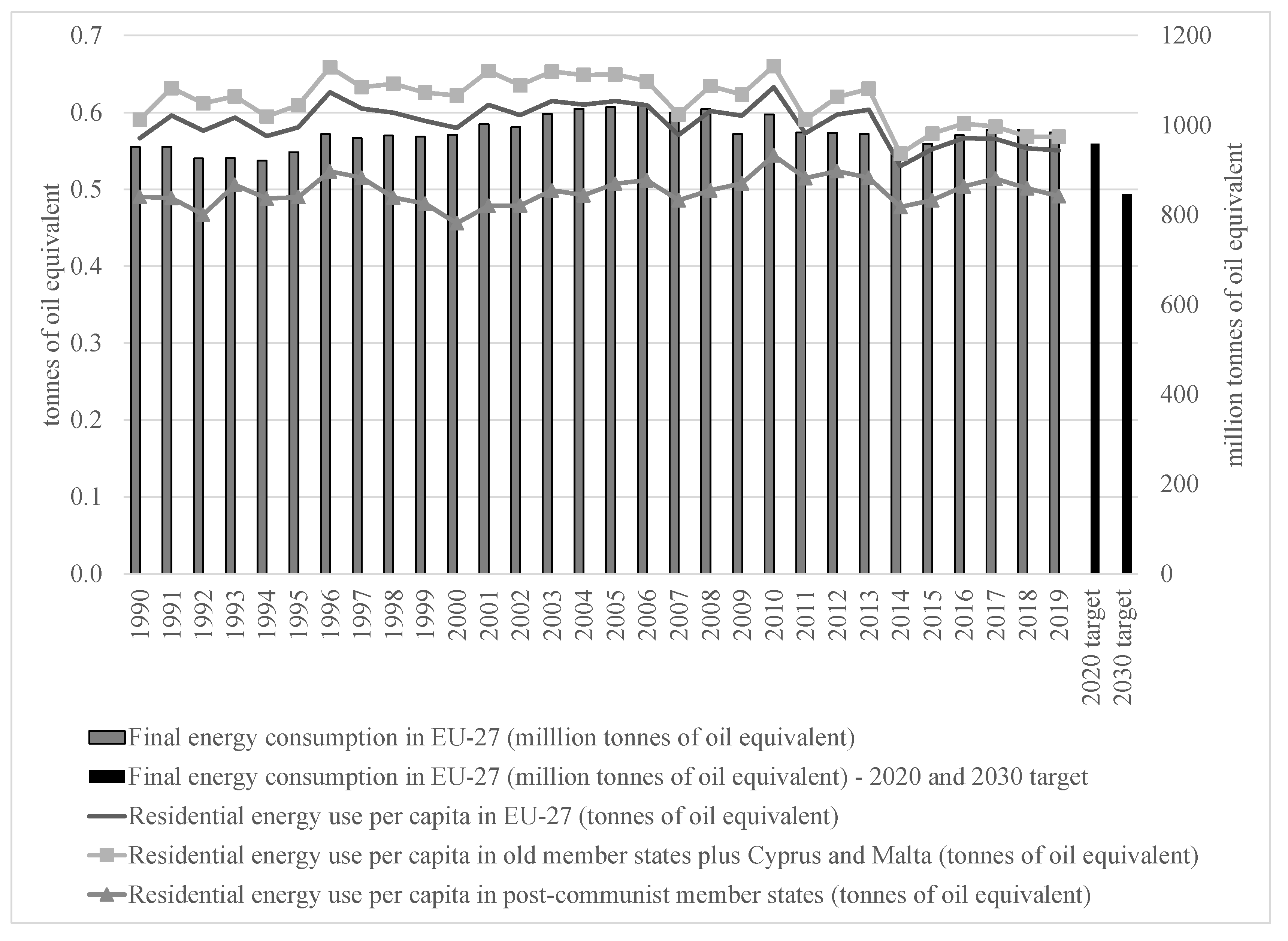
4.2. Scenario Analysis—Creating an Equilibrium in Energy Use and Human Well-Being
5. Conclusions
Author Contributions
Funding
Data Availability Statement
Acknowledgments
Conflicts of Interest
Appendix A


References
- European Commission. “Fit for 55”: Delivering the EU’s 2030 Climate Target on the Way to Climate Neutrality. COM/2021/550 Final; European Commission: Brussel, The Netherland, 2021; p. 15.
- Measuring Convergence. Available online: https://www.eurofound.europa.eu/topic/measuring-convergence (accessed on 6 May 2022).
- Ridao-Cano, C.; Bodewig, C. Growing United: Upgrading Europe’s Convergence Machine: Overview; World Bank Group: Washington, DC, USA, 2018. [Google Scholar]
- Bouzarovski, S.; Tirado Herrero, S. The Energy Divide: Integrating Energy Transitions, Regional Inequalities and Poverty Trends in the European Union. Eur. Urban Reg. Stud. 2017, 24, 69–86. [Google Scholar] [CrossRef] [PubMed]
- Sebestyénné Szép, T. Energy Convergence of the European Union toward 2020. Deturope 2016, 8, 20. [Google Scholar] [CrossRef]
- Evans, J.; Hunt, L.C. International Handbook on the Economics of Energy; Reprint edition; Edward Elgar Pub.: Cheltenham, UK, 2011; ISBN 978-0-85793-825-1. [Google Scholar]
- Ouedraogo, N.S. Energy Consumption and Human Development: Evidence from a Panel Cointegration and Error Correction Model. Energy 2013, 63, 28–41. [Google Scholar] [CrossRef]
- European Commission. Europe 2020 Targets 2017. Available online: https://ec.europa.eu/info/energy-climate-change-environment/overall-targets-and-reporting/2020-targets_en (accessed on 8 September 2022).
- Eurostat Database—Eurostat. Available online: https://ec.europa.eu/eurostat/data/database (accessed on 1 February 2021).
- Szép, T.; Tóth, G.; LaBelle, M.C. Farewell to the European Union’s east-west divide: Decoupling energy lifts the well-being of households, 2000–2018. Reg. Stat. 2022, 12, 159–190. [Google Scholar] [CrossRef]
- Szlávik, J.; Sebestyénné Szép, T. Delinking of Energy Consumption and Economic Growth in the Visegrad Group. Geogr. Tech. 2017, 12, 139–149. [Google Scholar] [CrossRef]
- Semieniuk, G.; Taylor, L.; Rezai, A.; Foley, D.K. Plausible Energy Demand Patterns in a Growing Global Economy with Climate Policy. Nat. Clim. Chang. 2021, 11, 313–318. [Google Scholar] [CrossRef]
- Csereklyei, Z.; Stern, D.I. Global Energy Use: Decoupling or Convergence? Energy Econ. 2015, 51, 633–641. [Google Scholar] [CrossRef]
- LaBelle, M.C. Energy Cultures. Technology, Justice, and Geopolitics in Eastern Europe; Edward Elgar Publishing: Northampton, MA, USA, 2020; ISBN 978-1-78897-575-9. [Google Scholar]
- Arto, I.; Capellán-Pérez, I.; Lago, R.; Bueno, G.; Bermejo, R. The Energy Requirements of a Developed World. Energy Sustain. Dev. 2016, 33, 1–13. [Google Scholar] [CrossRef]
- Brecha, R.J. Threshold Electricity Consumption Enables Multiple Sustainable Development Goals. Sustainability 2019, 11, 5047. [Google Scholar] [CrossRef]
- Jacmart, M.C.; Arditi, M.; Arditi, I. The World Distribution of Commercial Energy Consumption. Energy Policy 1979, 7, 199–207. [Google Scholar] [CrossRef]
- Jacobson, A.; Milman, A.D.; Kammen, D.M. Letting the (Energy) Gini out of the Bottle: Lorenz Curves of Cumulative Electricity Consumption and Gini Coefficients as Metrics of Energy Distribution and Equity. Energy Policy 2005, 33, 1825–1832. [Google Scholar] [CrossRef]
- Pasternak, A.D. Global Energy Futures and Human Development: A Framework for Analysis; U.S. Department of Energy, Lawrence Livermore National Laboratory: Livermore, CA, USA, 2000. [Google Scholar]
- Steinberger, J.K.; Roberts, J.T. From Constraint to Sufficiency: The Decoupling of Energy and Carbon from Human Needs, 1975–2005. Ecol. Econ. 2010, 70, 425–433. [Google Scholar] [CrossRef]
- Wu, Q.; Maslyuk, S.; Clulow, V. Energy Consumption Inequality and Human Development. Energy Effic. 2012, 18, 1398–1409. [Google Scholar]
- European Climate Foundation. Cambridge Econometrics Exploring the Trade-Offs in Different Paths to Reduce Transport and Heating Emissions in Europe. Available online: https://www.transportenvironment.org/discover/exploring-the-trade-offs-in-different-paths-to-reduce-transport-and-heating-emissions-in-europe/ (accessed on 6 May 2022).
- Sanchez-Guevara, C.; Núñez Peiró, M.; Taylor, J.; Mavrogianni, A.; Neila González, J. Assessing Population Vulnerability towards Summer Energy Poverty: Case Studies of Madrid and London. Energy Build. 2019, 190, 132–143. [Google Scholar] [CrossRef]
- Thomson, H.; Simcock, N.; Bouzarovski, S.; Petrova, S. Energy Poverty and Indoor Cooling: An Overlooked Issue in Europe. Energy Build. 2019, 196, 21–29. [Google Scholar] [CrossRef]
- Horta, A. Automobility and Oil Vulnerability: Unfairness as Critical to Energy Transitions. Nat. Cult. 2020, 15, 134–145. [Google Scholar] [CrossRef]
- Martiskainen, M.; Sovacool, B.K.; Lacey-Barnacle, M.; Hopkins, D.; Jenkins, K.E.H.; Simcock, N.; Mattioli, G.; Bouzarovski, S. New Dimensions of Vulnerability to Energy and Transport Poverty. Joule 2021, 5, 3–7. [Google Scholar] [CrossRef]
- Bouzarovski, S. Energy Poverty Policies at the EU Level. In Energy Poverty: (Dis)Assembling Europe’s Infrastructural Divide; Bouzarovski, S., Ed.; Springer International Publishing: Cham, Switzerland, 2018; pp. 41–73. ISBN 978-3-319-69299-9. [Google Scholar]
- Arto, I.; Capellán, I.; Lago, R. The Energy Footprint of Human Development. XIV Jorn. Econ. Crítica 2014, 134–151. Available online: http://www5.uva.es/jec14/comunica/A_EEMA/A_EEMA_6.pdf (accessed on 8 September 2022).
- Martínez, D.M.; Ebenhack, B.W. Understanding the Role of Energy Consumption in Human Development through the Use of Saturation Phenomena. Energy Policy 2008, 36, 1430–1435. [Google Scholar] [CrossRef]
- Mazur, A. Does Increasing Energy or Electricity Consumption Improve Quality of Life in Industrial Nations? Energy Policy 2011, 39, 2568–2572. [Google Scholar] [CrossRef]
- Nadimi, R.; Tokimatsu, K. Modeling of Quality of Life in Terms of Energy and Electricity Consumption. Appl. Energy 2018, 212, 1282–1294. [Google Scholar] [CrossRef]
- Tran, N.V.; Tran, Q.V.; Do, L.T.T.; Dinh, L.H.; Do, H.T.T. Trade off between Environment, Energy Consumption and Human Development: Do Levels of Economic Development Matter? Energy 2019, 173, 483–493. [Google Scholar] [CrossRef]
- Akizu-Gardoki, O.; Bueno, G.; Wiedmann, T.; Lopez-Guede, J.M.; Arto, I.; Hernandez, P.; Moran, D. Decoupling between Human Development and Energy Consumption within Footprint Accounts. J. Clean. Prod. 2018, 202, 1145–1157. [Google Scholar] [CrossRef]
- Steinberger, J.K.; Roberts, J.T. Across a Moving Threshold: Energy, Carbon and the Efficiency of Meeting Global Human Development Needs; Klagenfurt University: Klagenfurt, Austria, 2009. [Google Scholar]
- Dias, R.A.; Mattos, C.R.; Balestieri, J.A.P. The Limits of Human Development and the Use of Energy and Natural Resources. Energy Policy 2006, 34, 1026–1031. [Google Scholar] [CrossRef]
- Krugmann, H.; Goldemberg, J. The Energy Cost of Satisfying Basic Human Needs. Technol. Forecast. Soc. Chang. 1983, 24, 45–60. [Google Scholar] [CrossRef]
- Assadzadeh, A.; Nategh, H. The Relationship between per Capita Electricity Consumption and Human Development Indices. In Proceedings of the 6th IASTEM International Conference, Berlin, Germany, 29 November 2015; pp. 1–7, ISBN 978-93-85832-50-5. [Google Scholar]
- Kanagawa, M.; Nakata, T. Assessment of Access to Electricity and the Socio-Economic Impacts in Rural Areas of Developing Countries. Energy Policy 2008, 36, 2016–2029. [Google Scholar] [CrossRef]
- Ray, S.; Ghosh, B.; Bardhan, S.; Bhattacharyya, B. Studies on the Impact of Energy Quality on Human Development Index. Renew. Energy 2016, 92, 117–126. [Google Scholar] [CrossRef]
- Jorgenson, A.K.; Alekseyko, A.; Giedraitis, V. Energy Consumption, Human Well-Being and Economic Development in Central and Eastern European Nations: A Cautionary Tale of Sustainability. Energy Policy 2014, 66, 419–427. [Google Scholar] [CrossRef]
- Pasten, C.; Santamarina, J.C. Energy and Quality of Life. Energy Policy 2012, 49, 468–476. [Google Scholar] [CrossRef]
- Sušnik, J.; Zaag, P. van der Correlation and Causation between the UN Human Development Index and National and Personal Wealth and Resource Exploitation. Econ. Res. Ekon. Istraživanja 2017, 30, 1705–1723. [Google Scholar] [CrossRef]
- Sweidan, O.D.; Alwaked, A.A. Economic Development and the Energy Intensity of Human Well-Being: Evidence from the GCC Countries. Renew. Sustain. Energy Rev. 2016, 55, 1363–1369. [Google Scholar] [CrossRef]
- Gaye, A. Access to Energy and Human Development; Human Development Report Office Occasional Paper: New York, NY, USA, 2007; Volume 25, p. 22. [Google Scholar]
- Pachauri, S.; Spreng, D. Energy Use and Energy Access in Relation to Poverty. Econ. Polit. Wkly. 2004, 39, 271–278. [Google Scholar]
- The Global Innovation Index 2018: Energizing the World with Innovation; Dutta, S.; Lanvin, B.; Wunsch-Vincent, S. (Eds.) World Intellectual Property Organization: Geneva, Switzerland, 2018; ISBN 979-10-95870-09-8. [Google Scholar]
- Leung, C.S.; Meisen, P. How Electricity Consumption Affects Social and Economic Development by Comparing Low, Medium and High Human Development Countries. Glob. Energy Netw. Inst. 2005, 12. Available online: http://www.geni.org/globalenergy/issues/global/qualityoflife/HDI-vs-Electricity-Consumption-2005-07-18.pdf (accessed on 8 September 2022).
- LaBelle, M.C.; Georgiev, A. The Socio-Political Capture of Utilities: The Expense of Low Energy Prices in Bulgaria and Hungary. 2016, p. 21. Available online: https://erranet.org/download/socio-political-capture-of-utilities-bulgaria-hungary (accessed on 8 September 2022).
- Weiner, C.; Szép, T. The Hungarian Utility Cost Reduction Programme: An Impact Assessment. Energy Strategy Rev. 2022, 40, 100817. [Google Scholar] [CrossRef]
- Nussbaum, M. Women and Human Development; Cambridge University Press: Cambridge, UK, 2000. [Google Scholar]
- The Quality of Life; Nussbaum, M.; Sen, A. (Eds.) WIDER Studies in Development Economics; Oxford University Press: Oxford, UK, 1993; ISBN 978-0-19-828797-1. [Google Scholar]
- UNDP Human Development Data (1990–2018)|Human Development Reports. Available online: http://hdr.undp.org/en/data (accessed on 4 June 2020).
- World Bank World Bank Open Data | Data. Available online: https://data.worldbank.org/ (accessed on 27 June 2020).
- Fan, Y.; Chen, J.; Shirkey, G.; John, R.; Wu, S.R.; Park, H.; Shao, C. Applications of Structural Equation Modeling (SEM) in Ecological Studies: An Updated Review. Ecol. Process. 2016, 5, 19. [Google Scholar] [CrossRef]
- Tarka, P. An Overview of Structural Equation Modeling: Its Beginnings, Historical Development, Usefulness and Controversies in the Social Sciences. Qual. Quant. 2018, 52, 313–354. [Google Scholar] [CrossRef] [PubMed]
- Wolfle, L.M. Strategies of Path Analysis. Am. Educ. Res. J. 1980, 17, 183–209. [Google Scholar] [CrossRef]
- Alwin, D.F.; Hauser, R.M. The Decomposition of Effects in Path Analysis. Am. Sociol. Rev. 1975, 40, 37–47. [Google Scholar] [CrossRef]
- Duncan, O.D. Path Analysis: Sociological Examples. Am. J. Sociol. 1966, 72, 1–16. [Google Scholar] [CrossRef]
- Tóth, G.; Kincses, Á. Regional Distribution of Immigrants in Hungary. Hung. Geogr. Bull. 2010, 59, 107–130. [Google Scholar]
- Tóth, G.; Kincses, Á. Regional Distribution of Immigrants in Hungary—An Analytical Approach. Migr. Lett. 2011, 8, 98–110. [Google Scholar] [CrossRef]
- Murray, J.M. R Tutorials for Applied Statistics. Available online: https://murraylax.org/rtutorials/ (accessed on 3 July 2020).
- Németh, N. Fejlődési tengelyek az új hazai térszerkezetben. ELTE Reg. Tudományi Tanulmányok 2009, 15, 151. [Google Scholar]
- Klem, L. Path Analysis. In Reading and Understanding Multivariate Statistics; American Psychological Association: Washington, DC, USA, 1995; pp. 65–97. ISBN 978-1-55798-273-5. [Google Scholar]
- Loehlin, J.C.; Beaujean, A.A. Latent Variable Models: An Introduction to Factor, Path, and Structural Equation Analysis, 5th ed.; Routledge: London, UK, 2016; p. 390. [Google Scholar]
- Székelyi, M.; Barna, I. Túlélőkészlet az SPSS-hez. Többváltozós Elemzési Technikákról Társadalomkutatók Számára. Negyedik Kiadás; Typotex Kft: Budapest, Hungary, 2008. [Google Scholar]


| Abbreviation | Indicator | Source |
|---|---|---|
| HDI | Human development index | [52] |
| POP | Population on 1 January—total (persons) | [9] |
| RES | Final energy consumption in households per capita (Final consumption—other sectors—households—energy use/Population on 1 January—total) (toe) | own calculation based on [9] |
| SHE | Share of households in final energy consumption (Final energy consumption in households/Final consumption for energy use) (%) | own calculation based on [9] |
| DIST | Inequality of income distribution [The ratio of total income received by the 20% of the population with the highest income (top quintile) to that received by the 20% of the population with the lowest income (lowest quintile); income must be understood as equivalised disposable income] (%) | [9] |
| URB | Urbanization (urban population, % of total population) | [53] |
| MAN | Manufacturing, value added (% of GDP) | [53] |
| GDP | GDP growth (Gross domestic product at market prices, 2010 = 100%) | [9] |
| FDI | Foreign direct investment, net inflows (% of GDP) | [53] |
| CO2 | Carbon dioxide emission per capita (ton) | [9] |
| MET | Methane emission per capita (ton) | [9] |
| NIT | Nitrous oxide emission per capita (ton) | [9] |
| REN | Share of renewable energy in gross final energy consumption (%) | [9] |
| HDD | Heating degree days (number) | [9] |
| CDD | Cooling degree days (number) | [9] |
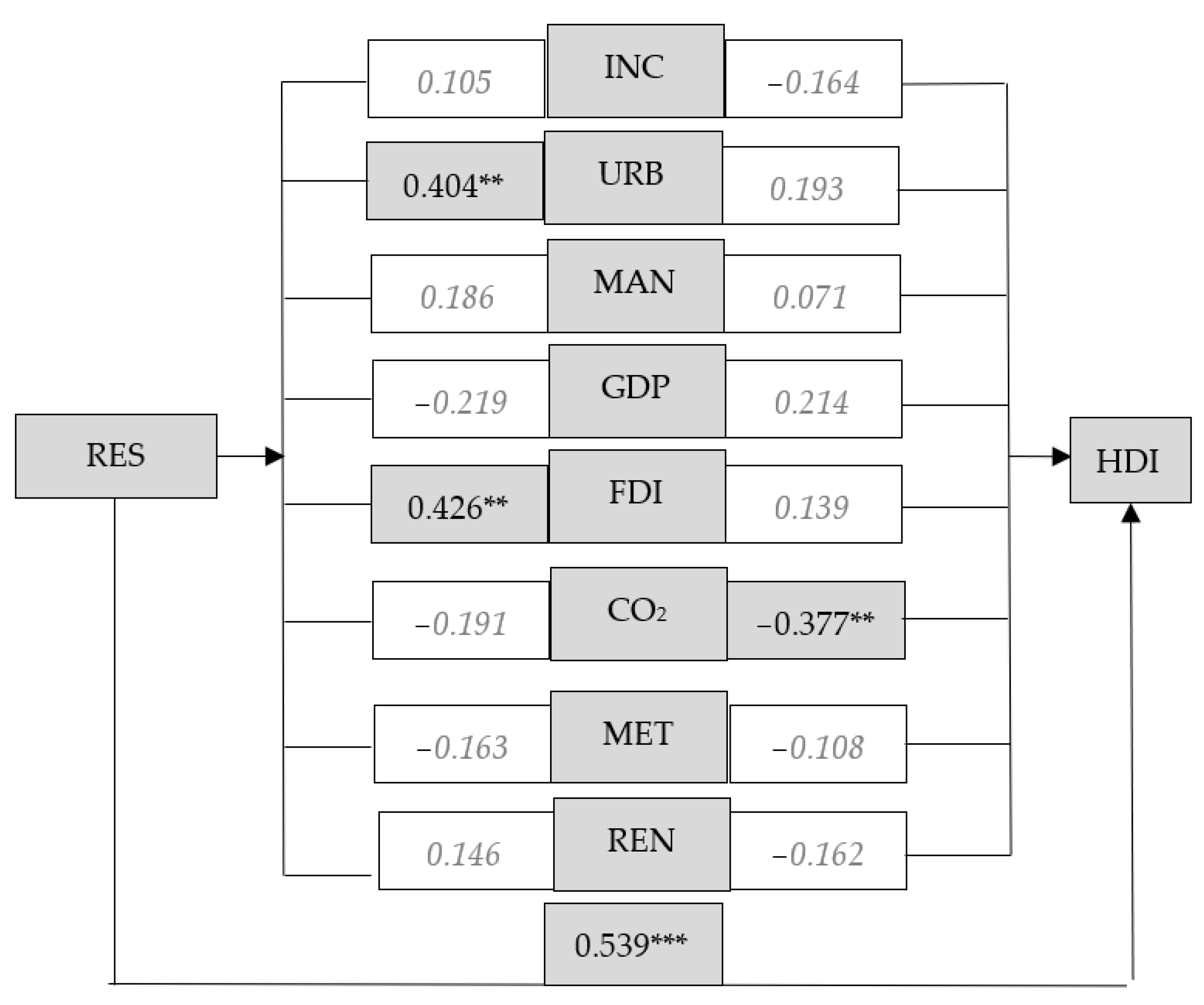
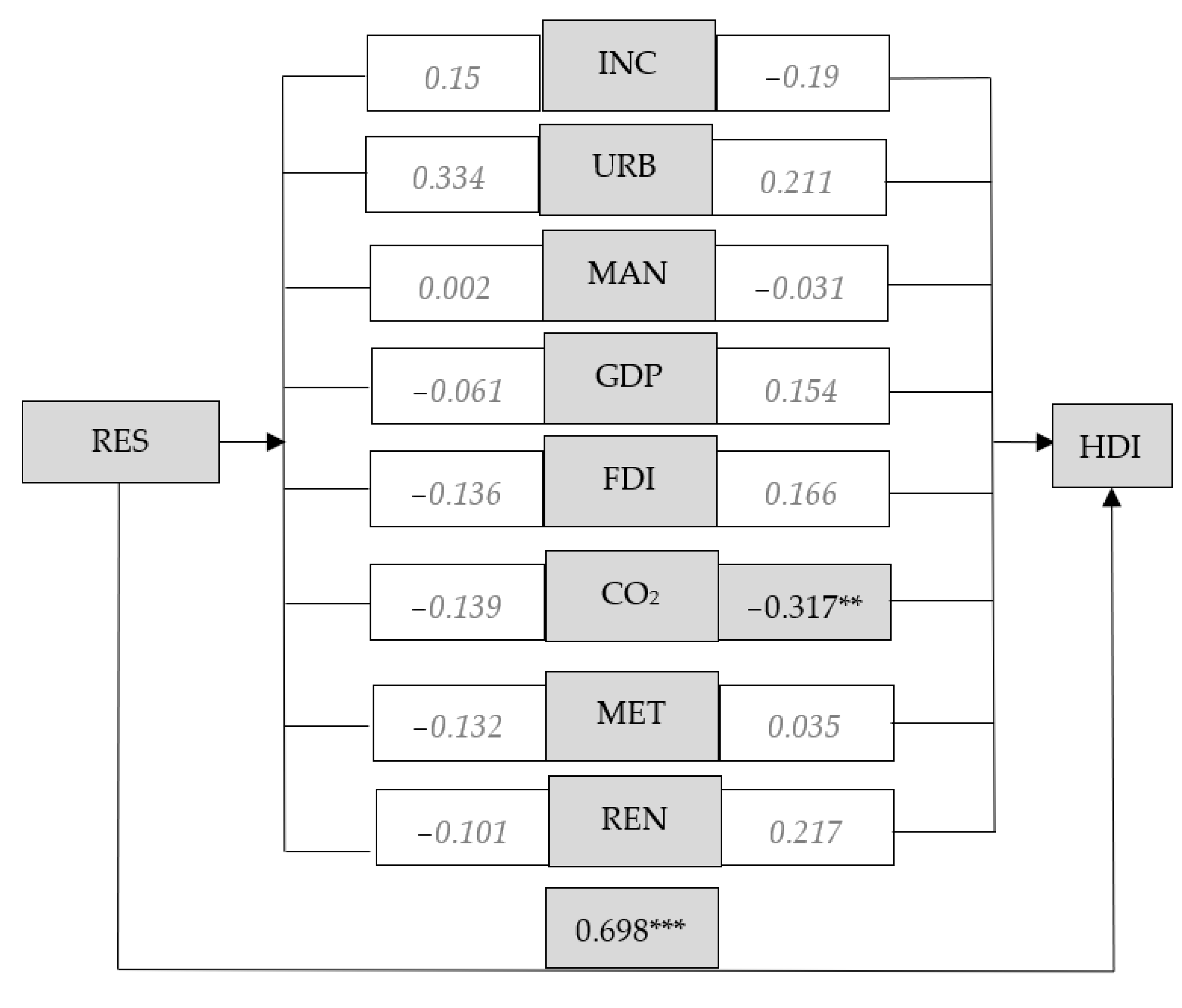
| Coefficients | Denomination | HDI, 2000 | Std. Error | HDI, 2008 | Std. Error | HDI, 2018 | Std. Error |
|---|---|---|---|---|---|---|---|
| β1 | RES | 0.595 *** | 0.047 | 0.698 *** | 0.027 | 0.319 * | 0.037 |
| β2 | INC | −0.164 | 0.007 | −0.190 | 0.006 | −0.221 | 0.004 |
| β3 | URB | 0.193 | 0.001 | 0.211 | 0.000 | 0.468 *** | 0.000 |
| β4 | MAN | 0.071 | 0.002 | −0.031 | 0.002 | 0.313 | 0.001 |
| β5 | GDP | 0.214 | 0.001 | 0.154 | 0.001 | −0.326 | 0.000 |
| β6 | FDI | 0.139 | 0.001 | 0.166 | 0.000 | 0.172 | 0.000 |
| β7 | CO2 | −0.377 ** | 0.002 | −0.317 ** | 0.002 | 0.149 | 0.002 |
| β8 | MET | −0.108 | 0.437 | 0.035 | 0.308 | 0.243 | 0.309 |
| β9 | REN | −0.162 | 0.001 | 0.217 | 0.001 | 0.073 | 0.000 |
| R2 | 0.58 | 0.61 | 0.67 |
| Coefficients | HDI, 2000 | Std. Error | HDI, 2008 | Std. Error | HDI, 2018 | Std. Error |
|---|---|---|---|---|---|---|
| Β | 0.691 *** | 0.033 | 0.714 *** | 0.026 | 0.574 *** | 0.031 |
| R2 | 0.456 | 0.490 | 0.303 |
| HDI, 2000 | HDI, 2008 | HDI, 2018 | |
|---|---|---|---|
| indirect | 0.152 | 0.027 | 0.255 |
| direct | 0.539 | 0.687 | 0.319 |
| Total | 0.691 | 0.715 | 0.574 |
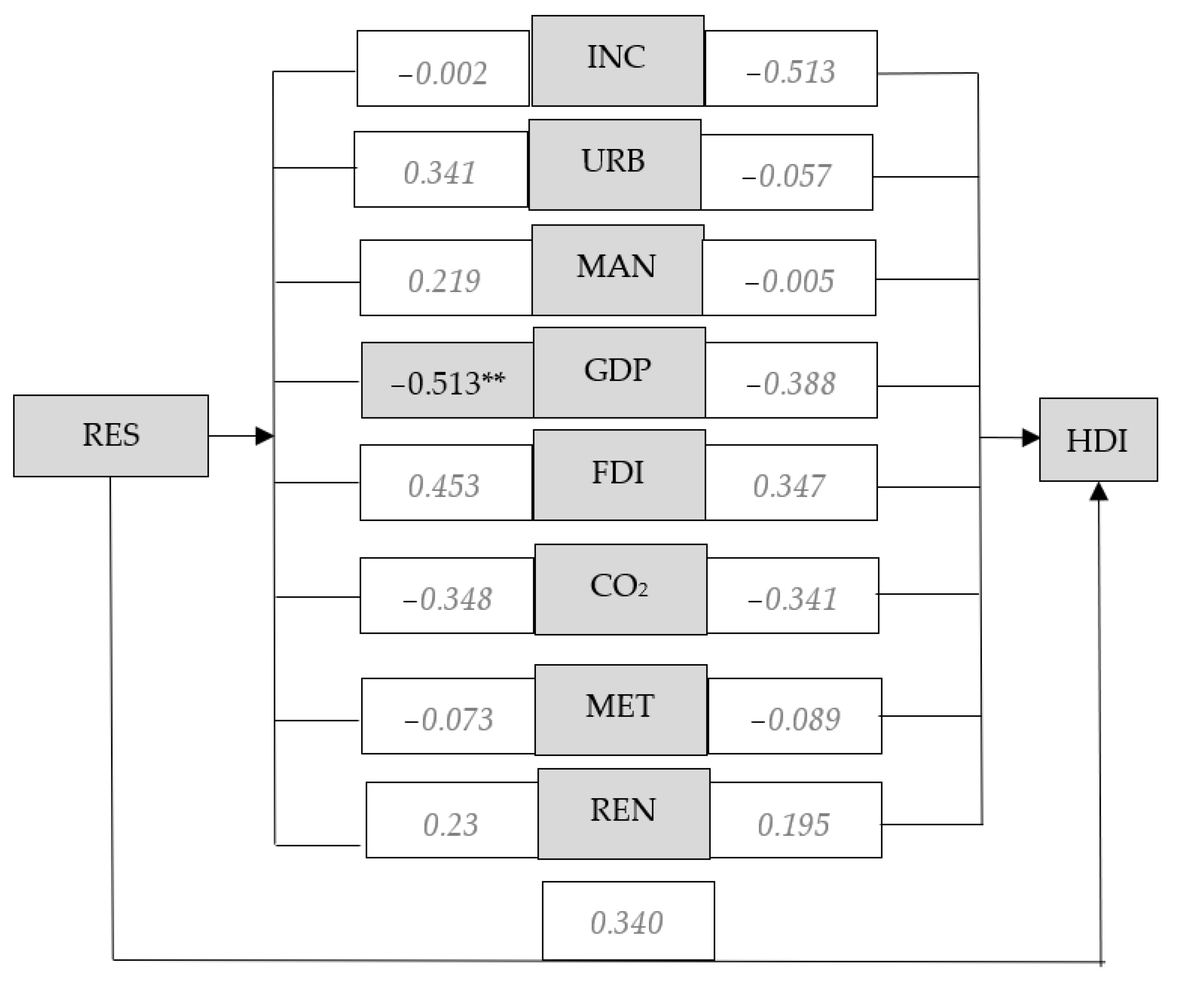
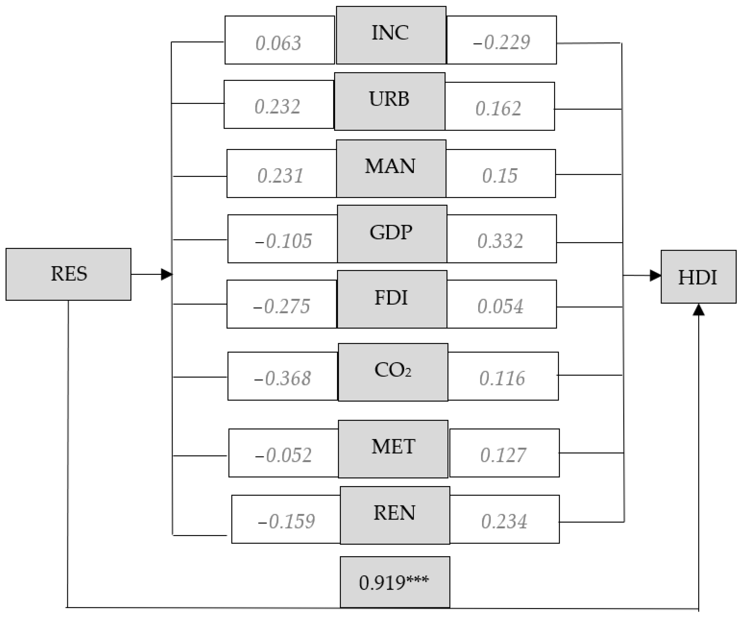
| Coefficients | Denomination | OMS | |||||
| 2000 | 2008 | 2018 | |||||
| HDI | Std. Error | HDI | Std. Error | HDI | Std. Error | ||
| β1 | RES | 0.340 | 0.035 | 0.919 *** | 0.019 | 0.152 | 0.036 |
| β2 | INC | −0.513 | 0.008 | −0.229 | 0.005 | −0.125 | 0.007 |
| β3 | URB | −0.057 | 0.001 | 0.162 | 0.000 | 0.307 | 0.001 |
| β4 | MAN | −0.005 | 0.002 | 0.150 | 0.001 | 0.675 ** | 0.001 |
| β5 | GDP | −0.388 | 0.001 | 0.332 | 0.001 | 0.295 | 0.000 |
| β6 | FDI | 0.347 | 0.001 | 0.054 | 0.000 | −0.139 | 0.000 |
| β8 | CO2 | −0.341 | 0.004 | 0.116 | 0.002 | 0.231 | 0.003 |
| β9 | MET | −0.089 | 0.266 | 0.127 | 0.198 | −0.323 | 0.385 |
| β10 | REN | 0.195 | 0.001 | 0.234 | 0.000 | 0.028 | 0.000 |
| R2 | 0.67 | 0.81 | 0.67 | ||||
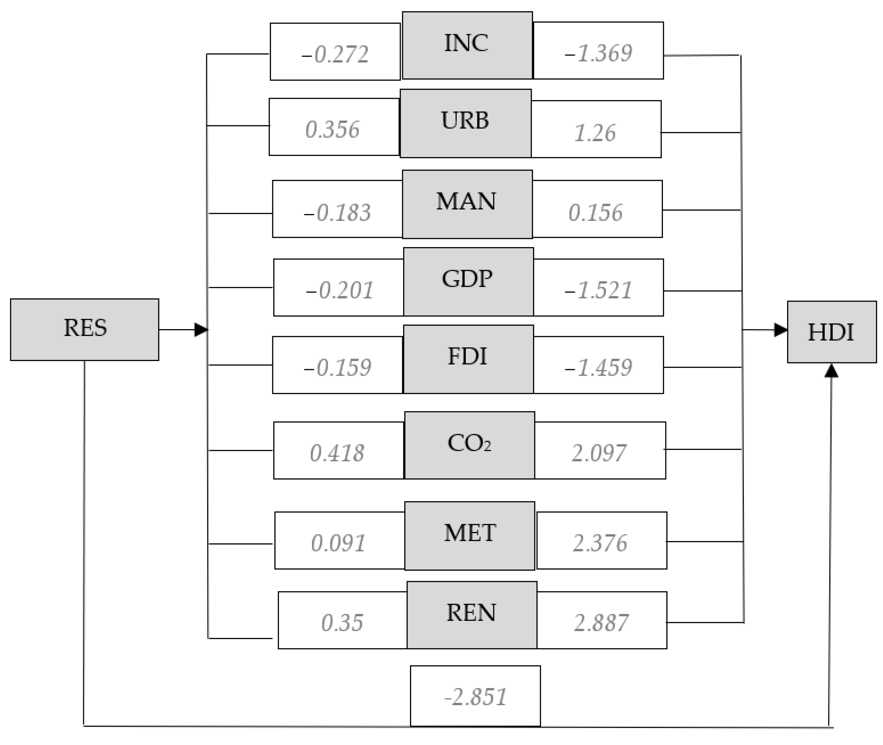
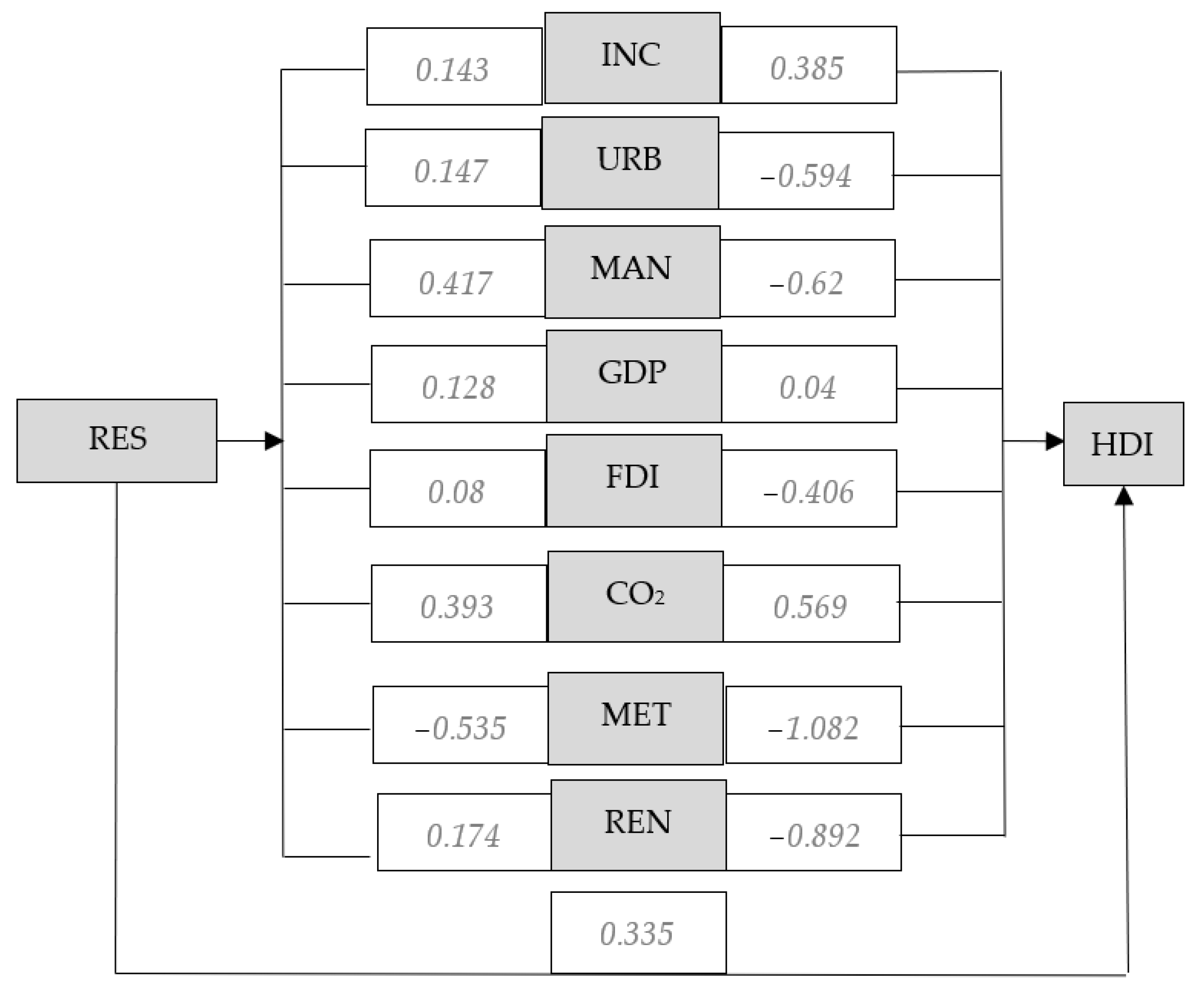
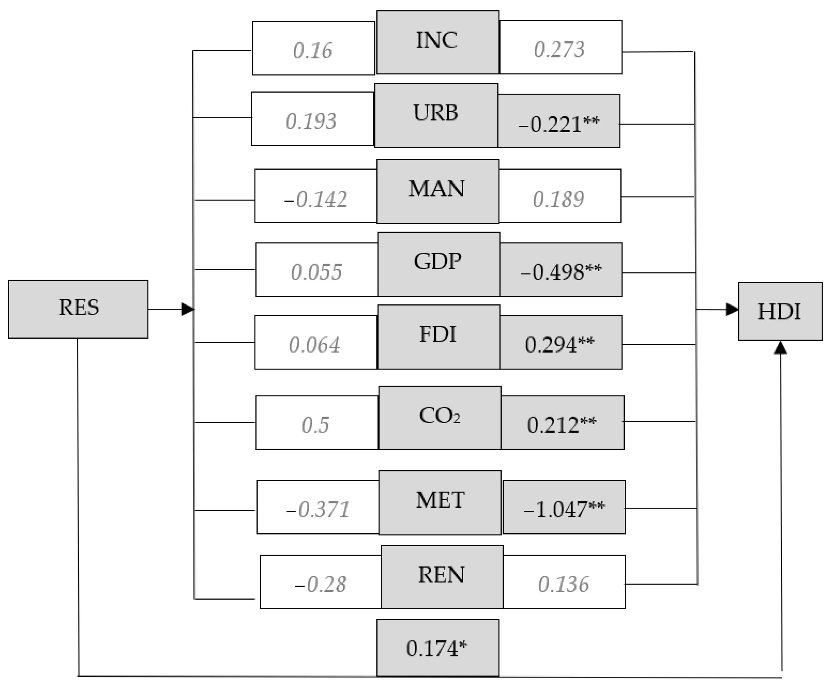
| Coefficients | Denomination | PCMS | |||||
| 2000 | 2008 | 2018 | |||||
| HDI | Std. Error | HDI | Std. Error | HDI | Std. Error | ||
| β1 | RES | 0.335 | 0.418 | 0.174 | 0.174 | −2.851 | 0.356 |
| β2 | INC | 0.385 | 0.045 | 0.273 | 0.273 | −1.369 | 0.017 |
| β3 | URB | −0.594 | 0.007 | −0.221 ** | −0.221 | 1.260 | 0.003 |
| β4 | MAN | −0.620 | 0.013 | 0.189 | 0.189 | 0.156 | 0.002 |
| β5 | GDP | 0.040 | 0.002 | −0.498 ** | −0.498 | −1.521 | 0.001 |
| β6 | FDI | −0.406 | 0.014 | 0.294 ** | 0.294 | −1.459 | 0.002 |
| β8 | CO2 | 0.569 | 0.015 | 0.212 ** | 0.212 | 2.097 | 0.007 |
| β9 | MET | −1.082 | 8.659 | −1.047 | −1.047 | 2.376 | 2.519 |
| β10 | REN | −0.892 | 0.004 | 0.136 | 0.136 | 2.887 | 0.004 |
| R2 | −0.29 | 1.00 | 0.81 | ||||
| Coefficients | OMS | |||||
| HDI, 2000 | Std. Error | HDI, 2008 | Std. Error | HDI, 2018 | Std. Error | |
| β | 0.846 *** | 0.018 | 0.841 *** | 0.018 | 0.695 *** | 0.024 |
| R2 | 0.696 | 0.686 | 0.446 | |||
| Coefficients | PCMS | |||||
| HDI, 2000 | Std. Error | HDI, 2008 | Std. Error | HDI, 2018 | Std. Error | |
| β | 0.663 ** | 0.074 | 0.596 ** | 0.058 | 0.585 * | 0.062 |
| R2 | 0.377 | 0.283 | 0.269 | |||
| OMS | PCMS | |||||
|---|---|---|---|---|---|---|
| HDI, 2000 | HDI, 2008 | HDI, 2018 | HDI, 2000 | HDI, 2008 | HDI, 2018 | |
| indirect | 0.507 | −0.078 | 0.543 | 0.329 | 0.422 | 3.433 |
| direct | 0.340 | 0.919 | 0.152 | 0.335 | 0.174 | −2.851 |
| Total | 0.846 | 0.840 | 0.695 | 0.663 | 0.596 | 0.585 |
Publisher’s Note: MDPI stays neutral with regard to jurisdictional claims in published maps and institutional affiliations. |
© 2022 by the authors. Licensee MDPI, Basel, Switzerland. This article is an open access article distributed under the terms and conditions of the Creative Commons Attribution (CC BY) license (https://creativecommons.org/licenses/by/4.0/).
Share and Cite
LaBelle, M.C.; Tóth, G.; Szép, T. Not Fit for 55: Prioritizing Human Well-Being in Residential Energy Consumption in the European Union. Energies 2022, 15, 6687. https://doi.org/10.3390/en15186687
LaBelle MC, Tóth G, Szép T. Not Fit for 55: Prioritizing Human Well-Being in Residential Energy Consumption in the European Union. Energies. 2022; 15(18):6687. https://doi.org/10.3390/en15186687
Chicago/Turabian StyleLaBelle, Michael Carnegie, Géza Tóth, and Tekla Szép. 2022. "Not Fit for 55: Prioritizing Human Well-Being in Residential Energy Consumption in the European Union" Energies 15, no. 18: 6687. https://doi.org/10.3390/en15186687
APA StyleLaBelle, M. C., Tóth, G., & Szép, T. (2022). Not Fit for 55: Prioritizing Human Well-Being in Residential Energy Consumption in the European Union. Energies, 15(18), 6687. https://doi.org/10.3390/en15186687